Abstract

We review the possibility to use the renormalons emerging in the perturbation series of the twist-2 part of the nonsinglet structure functions $F_{L}$, $F_{2}$, $F_{3}$, and $g_{1}$ to make approximate predictions for the magnitude of the appertaining twist-4 corrections.

1 Introduction

The precision of deep inelastic scattering experiments nowadays allows for the disentanglement of genuine twist-4 corrections to unpolarized structure functions. While the twist-2 parton density has a simple probabilistic interpretation in the parton model, genuine twist-4 corrections can be seen as multiple particle correlations between quarks and gluons. For example the twist-4 correction to the Bjorken sum rule $f^{(2)}$ can be interpreted as the interaction of the induced color electric $E_{A}^{\sigma}$ and color magnetic fields $B_{A}^{\sigma}$ of a single quark and the corresponding nucleon remnant [1]:

$$\langle pS|-B_{A}^{\sigma}j_{A}^{0}+(\vec{j}_{A}\times\vec{E}_{A})^{\sigma}|pS\rangle=2m_{N}^{2}f^{(2)}S^{\sigma}\quad,$$ (1)

where $m_{N}$ is the nucleon mass, $p$ the momentum and $S$ the spin of the incoming nucleon. Despite of the capability to isolate at least for the unpolarized case the twist-4 contributions to structure functions in experiments [2], on the theoretical side the description of higher-twist contributions is still not satisfactory. Even though the operator product expansion is possible for inclusive quantities its technical applicability is restricted to the lowest moments of the structure functions [3]. The best and physically most stringent approach to estimate the magnitude of the matrix elements of the twist-4 operators, the lattice gauge theory, suffers from the problem of operator mixing which still has to be solved. In this approach up to now higher-twist corrections were calculated only in cases where such a mixing is forbidden by some quantum numbers, e.g. as in the case of the twist-3 correction to the Bjorken sum rule [4]. In total, we are far away from getting hold of the twist-4 contribution to all moments and consequently from a description which gives the $x$-dependent contribution of the twist-4 correction to the whole structure function.

The renormalon approach cannot really cure this problem because of its approximative and partially very speculative nature, but it offers a well defined model. This model was applied to the nonsinglet structure functions either in terms of the massive gluon scheme or the running coupling scheme which in general have an one to one correspondence [5]. Empirically, it has proven to be quite successful to reproduce at least in the large-$x$ range the $x$ dependence of the twist-4 correction to the unpolarized structure functions [6, 7, 8]. The success of this model is nowadays referred to as the ‘ultraviolet dominance’ of twist-4 operators [9].

In the following first two sections we will shortly outline the definition and the basic features of the renormalon in QCD and the technique of naive nonabelianization (NNA), which allows to reduce the calculational effort necessary to the mere summation of vacuum polarization bubbles. We also comment on the very important question of the scheme dependence of the renormalon and in the last section we want to discuss the renormalon contribution to the structure functions $g_{1}$, $F_{L}$, $F_{2}$, and $F_{3}$ in detail and compare it to the measured data. For a review and references to the classical papers on renormalons see [10].

2 What are Renormalons?

The operator product expansion predicts that a moment of an unpolarized structure function $F$ ($F=F_{2},F_{L},F_{3}$) admits up to ${\cal O}(1/Q^{4})$ the following general form:

$$M_{n}(F) := \int_{0}^{1}dxx^{n}F(x)$$ (2)

$$= C_{n}a_{n}^{twist=2}+\frac{1}{Q^{2}}\left[M^{2}C_{n}^{\prime}b_{n}^{twist=2}+C^{(1)}_{n}b_{1,n}^{twist=4}+C^{(2)}_{n}b_{2,n}^{twist=4}+..\right]\;.$$

Each Wilson Coefficient (e.g. $C_{n}$) can be written as an asymptotic series in the strong coupling constant.

$$C_{n}=C_{n}(Q^{2}/\mu^{2},a_{s})=\sum_{m=0}^{m_{0}-1}C_{m,n}a_{s}^{m}+\Delta R;\;a_{s}=\frac{\alpha_{s}}{4\pi}\;.$$ (3)

$m_{0}$ corresponds to the minimal term of the series and is given by the condition

$$\left|\frac{a_{s}C_{n,m_{0}}}{C_{n,m_{0}-1}}\right|>1\;\Rightarrow\Delta R=C_{n,m_{0}}a_{s}^{m_{0}}\;.$$ (4)

In a certain approximation the Wilson coefficient can be evaluated to all orders, i.e. when we take the numbers of fermions to infinity, $N_{F}\to\infty$. One then can derive a closed formula for $C_{m,n}$ for all $m$ and $n$. Only the flavor nonsinglet case has been considered so far. The Borel-transformed series

$$B[C_{n}](s)=\sum_{m}C_{n,m}\frac{1}{m!}\left(\frac{s}{\beta_{0}}\right)^{m}\;,$$ (5)

with $\beta_{0}=-\frac{1}{4\pi}\frac{2}{3}N_{F}$ $(N_{F}\to\infty)$, has the pole structure:

$$B[C_{n}](s) = \left(\frac{\mu^{2}e^{-C}}{Q^{2}}\right)^{s}\left(...+\frac{p_{n}^{IR_{2}}}{2-s}+\frac{p_{n}^{IR_{1}}}{1-s}+\frac{p_{n}^{UV_{1}}}{1+s}+\frac{p_{n}^{UV_{2}}}{2+s}+...\right)\;,$$ (6)

reflecting the fact that the QCD-perturbation series is not Borel summable. The $p_{n}^{UV_{j}}$ and $p_{n}^{IR_{j}}$ define residua of ultraviolet- and infrared-renormalon poles, respectively. The existence of infrared-renormalon poles makes the unambiguous reconstruction of the summed series from its Borel representation impossible. $C$ is the finite part of the fermion loop insertion into the gluon propagator equal to $-5/3$ in the $\rm\overline{MS}$ scheme. The Borel representation $B[C_{n}]$ can be used as the generating function for the fixed order coefficients

$$C_{n,m}=\beta_{0}^{m}\frac{d^{m}}{ds^{m}}B[C_{n}](s)\Bigg{|}_{s=0}\;,$$ (7)

which implies for large $m$ the following asymptotic behavior of the coefficient functions

$$C_{n,m}^{IR_{1}} \sim p_{n}^{IR_{1}}\left(\frac{\mu^{2}e^{-C}}{Q^{2}}\right)m!\beta_{0}^{m}$$

$$C_{n,m}^{IR_{2}} \sim p_{n}^{IR_{2}}\left(\frac{\mu^{2}e^{-C}}{Q^{2}}\right)^{2}m!\beta_{0}^{m}\left(\frac{1}{2}\right)^{m}$$

$$C_{n,m}^{UV_{1}} \sim p_{n}^{UV_{1}}\left(\frac{\mu^{2}e^{-C}}{Q^{2}}\right)^{-1}m!\beta_{0}^{m}(-)^{m}$$

$$C_{n,m}^{UV_{2}} \sim p_{n}^{UV_{2}}\left(\frac{\mu^{2}e^{-C}}{Q^{2}}\right)^{-2}m!\beta_{0}^{m}\left(-\frac{1}{2}\right)^{m}\;.$$ (8)

The infrared renormalon pole nearest to the origin of the Borel plane dominates the asymptotic expansion. Its name originates from the fact that in asymptotically free theories the origin of the factorial divergence of the series can be traced to the integration over the low momentum region of Feynmann diagrams:

$$\sum_{m=0}^{\infty}\alpha_{s}(Q^{2})^{m+1}m!\frac{1}{j}\left(\frac{\beta_{0}}{j}\right)^{m}=\int_{0}^{Q^{2}}\frac{dk^{2}}{k^{2}}\left(\frac{k^{2}}{Q^{2}}\right)^{j}\alpha_{s}(k^{2})\;,$$ (9)

with

$$\alpha(k^{2})=\frac{\alpha(Q^{2})}{1+\beta_{0}\alpha(Q^{2})\ln(k^{2}/Q^{2})}\quad.$$ (10)

The uncertainty of the asymptotic perturbation series can be either estimated by calculating the minimal term in the expansion (3) or by taking the imaginary part (divided by $\pi$) of $B[C_{n}](s)$ [11]:

$$\Delta R = \frac{1}{\pi}{\cal I}\frac{1}{\beta_{0}}\int_{0}^{\infty}ds\exp\left(\frac{-s}{\beta_{0}\alpha_{s}}\right)B[R](s)$$ (11)

$$\sim \pm p_{n}^{IR_{1}}\frac{1}{\beta_{0}}\left(\frac{\Lambda_{C}^{2}e^{-C}}{Q^{2}}\right)\;.$$

The undetermined sign is due to the two possible contour integrations, below or above the pole.

In a physical quantity the infrared-renormalon ambiguities have to cancel, against similar ambiguities in the definition of twist-4 operators such that in principle only the sum of both is well defined. Operators of higher-twist and therefore higher dimension may exhibit power-like UV divergences, and the corresponding ambiguity can be extracted as the quadratic UV divergence of the twist-4 operator. Because of this cancellation, the IR renormalon is in a one-to-one correspondence with the quadratic UV divergence of the twist-4 operator. Taking the IR renormalon contibution as an estimate of real twist-4 matrix elements is therefore equivalent to the assumption that the latter are dominated by their UV divergent part.

In practice, the all-orders calculation can be performed only in the large-$N_{F}$ limit, which corresponds to the QED case, where it produces an ultraviolet renormalon. To make the connection to QCD one uses the ’Naive Non Abelianization’ (NNA) recipe [12] and substitutes for the QED one-loop $\beta$-function the corresponding QCD expression.

$$\beta_{0}^{\rm limit} = -\frac{1}{4\pi}\frac{2}{3}N_{F}\rightarrow\frac{1}{4\pi}\left(11-\frac{2}{3}N_{F}\right)\;.$$ (12)

The positive sign of $\beta_{0}$ in QCD produces an infrared-renormalon. While no satisfactory justification for this approximation is known so far, it has proven to work quite well in low orders were comparison to the known exact coefficients in the ${\rm\overline{MS}}$ scheme is possible [13]. Despite its phenomenological success in describing the shape of higher-twist corrections to various QCD observables, one should be aware of conceptual limitations of this approach. As the renormalon contribution is constructed from twist-2 parton distributions only, it really has no sensitivity to the intrinsic non-perturbative twist-4 nucleon structure. For example the ratio of the n-th moment $M_{n}$ of the twist-4 renormalon prediction to a structure function and the n-th moment of the twist-2 part of the structure functions itself is by construction the same for different hadrons:

$$\frac{M_{n}^{twist-4}}{M_{n}^{twist-2}}\Bigg{|}_{\rm hadron1}-\frac{M_{n}^{twist-4}}{M_{n}^{twist-2}}\Bigg{|}_{\rm hadron2}=0\;,$$ (13)

which is definitely not necessarily the case in reality.

As far as the scheme dependence of the renormalon model is concerned, its prediction for the magnitude of the mass scale of higher-twist corrections $\sim\Lambda_{C}^{2}e^{-C}$ is scheme invariant in the large-$N_{F}$ limit only. On the other hand, once one takes this scale to be a fit parameter, where the magnitude of this fit parameter depends on the process under consideration, this scheme dependence disappears. Even in this case, however, the mass scale still depends on the scheme used to determine perturbative corrections to the twist-2 part. Thus one can only say that the renormalon model is just a very economical way of estimating higher-twist contributions in the situation when their exact theory has not yet been constructed. In addition, in cases where the operator product expansion is not directly applicable, like in Drell Yan, the renormalon can still trace power corrections and give an approximation of their magnitude.

In order to demonstrate how it works, let us consider the phenomenologically important case of twist-4 corrections to the Bjorken sum-rule:

$$\int_{0}^{1}dxg_{1}^{p-n}(x,Q^{2}) = \frac{1}{6}\frac{g_{A}}{g_{V}}+\mu\frac{GeV^{2}}{Q^{2}}+{\cal O}(1/Q^{4})$$

$$g_{A}/g_{V} = -1.2601\pm 0.0025\qquad\cite[cite]{[\@@bibref{}{PPBL96}{}{}]}\;.$$ (14)

The $1/Q^{2}$ power corrections consist of target-mass corrections, a twist-3 and a twist-4 part [15]. Only the twist-4 part can be traced by the renormalon ambiguity because this is the only operator which can mix with the spin-1, twist-2 axial current operator. Table 1 contains results of various approaches employed so far. A QCD-sum rule calculation is described in [16, 1]. Due to the high dimension of the corresponding operator the error arising from the sum rule calculation is large, typically of the order of 50 percent. Another possibility is the MIT-Bag model, which however lacks explicit Lorentz invariance. As long as an unambiguous field-theoretical definition of twist-4 matrix elements does not exist, only the twist-3 part of the coefficient $\mu$ can be calculated on the lattice [4]. Recently the twist-4 matrix element has been estimated within the framework of the chiral soliton model [18], providing a semi classical description. The prediction of the renormalon model, which attributes the whole power correction to the twist-4 operator, is in an order-of-magnitude agreement with results of the other methods. The twist-4 contribution has also been estimated from the experimental data [19], yielding a value within a large error which is also in agreement with all the other methods as far as the order of magnitude is concerned, but predicting a positive sign in contrast to all calculations except the bag-model calculation. Note, that due to its nature as an ambiguity in the twist-2 calculation the renormalon prediction is not capable to fix the absolute sign.

Having the calculational efforts of sum rules and lattice QCD in mind, it might be an interesting idea to get a zero-order guess of the size of the twist-4 corrections by looking at the ambiguity in the expansion of the twist-2 part.

method	value	reference
sum rule	$\mu=0.003\pm 0.008$	[1]
	$\mu_{twist-4}=-0.0094$	[1]
bag model	$\mu=0.027$	[17]
	$\mu_{twist-4}=0.014$	[17]
chiral soliton model	$\mu_{twist-4}=-0.013$	[18]
extraction from data	$\mu_{twist-4}=0.012\pm 0.037$	[19]
renormalon	$\mu=\pm 0.017$	[20]

Table 1: Higher-twist contributions to the Bjorken sum rule

3 The renormalon contribution to $F_{L}$,$F_{2}$,$F_{3}$, and $g_{1}$

Finally we will discuss the application of the renormalon model to the $x$ dependence of DIS structure functions. Indeed the real success of the renormalon method in DIS - as noticed in [6, 7] - is their capability to reproduce the $x$ dependence of measured higher-twist contributions. The absolute magnitude of the renormalon contribution can be either left as a fit parameter, taken from the NNA-calculation, or taken as an universal constant as done in the gluon scheme of [21].

We once more regard the nonsinglet part of the structure function $g_{1}$ [22]. In Fig. 1 $xg_{1}$ is plotted from the parton distribution set Gehrman/Stirling Gluon A [23] plus/minus the renormalon predicted twist-4 contribution, which is on the percent level. The dotted line gives the renormalon prediction again, amplified by a factor of 10. It becomes visible that the curve contains a zero at $x\approx 0.7$, a feature which is a very definite and clear prediction and should be confronted to experimental data, if a precision on the precent level was reached.

As to $F_{L}$ [6], we plot in Fig. 2 the appertaining renormalon prediction to the twist-4 operator (short dashed line). The target mass corrections taken from [24] are plotted by a dotted line. The sum of both is combined to the long dashed line and has to be compared to the experminental fit by [25, 26] (solid line). The $x$ dependence is quite well approximated by the renormalon approach, which predicts well the measured $x$ dependence although the absolute magnitude is smaller than what is suggested by the experimental fit, but the $x$ dependence is described in an acceptable way.

As to the notation for the twist-4 corrections of the structure functions $F_{2}$ and $F_{3}$ we write ($i=2,3$)

$$F_{i}(x,Q^{2}) = F_{i}^{(LT)}(x,Q^{2})+\frac{1}{Q^{2}}h_{i}(x)=F_{i}^{(LT)}(x,Q^{2})\left(1+\frac{C_{i}(x)}{Q^{2}}\right)\;.$$ (15)

In the case of $F_{2}$ the good agreement between the $x$ behavior of the nonsinglet renormalon contribution and the deuteron and proton twist-4 contribution (see Fig 3) to $F_{2}$ has been noticed in [7]. It is remarkable that the uncalculated pure singlet part seems to be small or proportional to the nonsinglet part. At least in the large-$x$ range, where gluons contribute only a minor part, this is understandable. If we calculate the absolute value of the renormalon contributions for $F_{2}$ (solid line) it falls short by a factor 2 or 3, compared with what seems to be required by the data [8].

The same behavior is found for the structure function $F_{3}$, where the twist-4 contribution is shown in Fig. 4. Again, if one is adjusting the absolute size of the renormalon contribution in the same way as it was done for $F_{2}$, the result is in the large-$x$ range in a good agreement with the data. Even more remarkable is the fact that the data indicate a change in sign in the large-$x$ region close to the one of the renormalon prediction.

4 Conclusions

The renormalon prescription provides a satisfactory description of the shape of the measured values of the twist-4 contributions at large $x$ in the cases studied so far, leaving the absolute normalization as a fit parameter. Empirically, it falls short by a factor 2 - 3 as to the measured magnitude of the finite twist-4 contributions, when it is calculated in the $\rm\overline{MS}$ scheme.

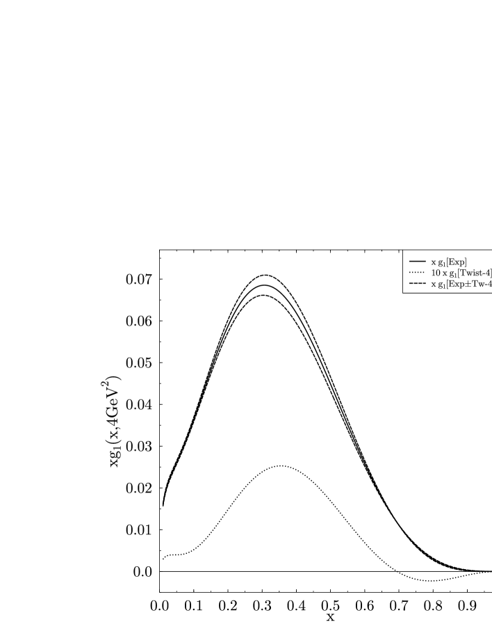
Figure 1: Experimental fit [23] for $g_{1}(x,4\,{\rm GeV}^{2})$ (full line). The estimate for the twist-4 correction is given explicitly multiplied by a factor of $10$ (dotted line). The correction was added and subtracted from the experimental values (dashed lines) ($\Lambda_{\overline{MS}}=200~{}{\rm MeV}$, $Q^{2}=4~{}{\rm GeV}$ and $N_{f}=4$).

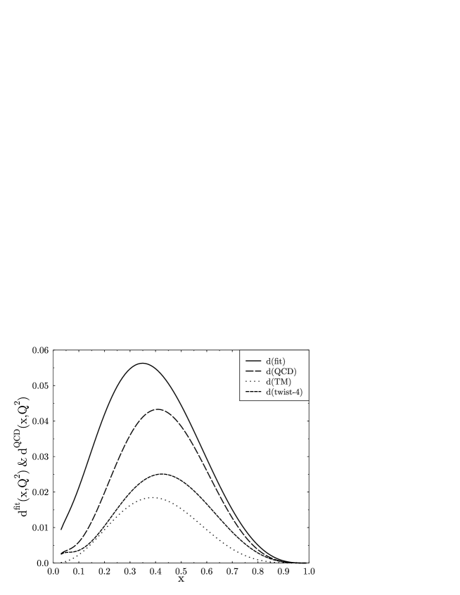
Figure 2: $F_{L}(x,Q^{2})=F_{L}^{twist-2}(x,Q^{2})+\frac{d(x,Q^{2})}{Q^{2}}$ $+{\cal O}(1/Q^{4})$. We have chosen $\Lambda_{\overline{MS}}=250~{}{\rm MeV}$, $Q^{2}=5~{}{\rm GeV}$ and $N_{f}=4$.

Figure 3: The solid line shows the renormalon model predictions for $C_{p}$ and $C_{d}$, which are indistinguishable, LO parameterization taken from [27]. The dashed line shows the fit, as in Ref. [7]. The filled and empty circles display the data for $C_{p}$ and $C_{d}$ according to Ref. [2], respectively.

Figure 4: Renormalon prediction for $xh_{3}(x)$ using the LO GRV [27] parametrization (solid line). The data points taken from Ref. [28] correspond to the NLO analysis, which provides the best fit of the higher-twist corrections. However, to be consitent within the renormalon approach the parton distribution sets used for the renormalon prediction have to be LO. The dashed line shows the prediction with the scale $\mu^{2}$ adjusted to the description of the coefficients $C_{p}$ and $C_{d}$, as in [7]. The dot-dashed line shows the original prediction of [7], obtained using the MRSA parametrization [29] normalized at $Q^{2}=10$ GeV².

References

- [1] E. Stein, P. Gornicki, L. Mankiewicz, and A. Schäfer, Phys. Lett. B343 (1995) 369, Phys. Lett. B353 (1995) 107.
- [2] M. Virchaux and A. Milsztajn, Phys. Lett. B274 (1992) 221.
-
[3]
E. V. Shuryak and A. I. Vainshtein, Nucl. Phys. B199 (1982) 451;
R. L. Jaffe and M. Soldate, Phys. Rev. D26 (1982) 49. - [4] M. Göckeler, R. Horsley, E. M. Ilgenfritz, H. Perlt, G. Schierholz A. Schiller, Phys. Rev. D53 (1996) 2317.
- [5] P. Ball, M. Beneke and V. M. Braun, Nucl. Phys. B452 (1995) 563.
- [6] E. Stein, M. Meyer-Hermann, L. Mankiewicz, A. Schäfer, Phys. Lett. B376 (1996) 177.
- [7] M. Dasgupta, B. R. Webber, Phys. Lett. B382 (1996) 273.
- [8] M. Maul, E. Stein, A. Schäfer, L. Mankiewicz, Phys. Lett. B401 (1997) 100.
- [9] M. Beneke, V. M. Braun, L. Magnea, Nucl. Phys. B497 (1997) 297.
-
[10]
M. Neubert, Phys. Rev. D51 (1995) 5924;
M. Beneke, V. M. Braun, Nucl. Phys. B454 (1995) 253 ;
R. Akhoury, V. I. Zakharov, Phys. Lett. B357 (1995) 646;
C. N. Lovett-Turner, C.J. Maxwell, Nucl. Phys. B452 (1995) 188;
N. V. Krasnikov, A. A. Pivovarov, Mod. Phys. Lett. A11 (1996) 835;
P. Nason, M. H. Seymour, Nucl. Phys. B454 (1995) 291;
P. Korchemsky, G. Sterman, Nucl. Phys. B437 (1995) 415.
- [11] V. M. Braun, QCD renormalons and higher-twist effects hep-ph 9505317, Mar 1995. 7pp. Talk given at 30th Rencontres de Moriond: QCD and High Energy Hadronic Interactions, Meribel les Allues, France, 19-25 Mar 1995. Published in Moriond 1995: Hadronic:271-278 (QCD161:R4:1995:V.2)
-
[12]
D. J. Broadhurst and A. G. Grozin, Phys. Rev. D52 (1995) 4082;
M. Beneke and V. M. Braun, Phys. Lett. B348 (1995) 513;
P. Ball, M. Beneke, V. M. Braun, Nucl. Phys. B452 (1995) 563;
M. Beneke, Nucl. Phys. B405 (1993) 424;
- [13] L. Mankiewicz, M. Maul, E. Stein Phys. Lett. B404 (1997) 345.
- [14] Particle properties, Phys. Rev. D54 (1996) 1.
- [15] B. Ehrnsperger, A. Schäfer, L. Mankiewicz, Phys. Lett. B323 (1994) 439.
- [16] I. I. Balitsky, V. M. Braun, and A. V. Kolesnichenko, Phys. Lett. B242 (1990) 245; Phys. Lett. B318 (1993) 648 (E).
- [17] X. Ji, P. Unrau, Phys. Lett. B333 (1994) 228.
- [18] J. Balla, M. V. Polyakov, C. Weiss (Ruhr U., Bochum), RUB-TPII-6-97, Jul 1997. 40pp. e-Print Archive: hep-ph/9707515
- [19] X. Ji, W. Melnitchouk, Phys. Rev. D56 (1997) 1.
-
[20]
M. Beneke and V. M. Braun, Nucl. Phys. B454 (1995), 253;
V.M. Braun (DESY).hep-ph 9505317, Mar 1995. 7pp. Talk given at 30th Rencontres de Moriond: QCD and High Energy Hadronic Interactions, Meribel les Allues, France, 19-25 Mar 1995. Published in Moriond 1995: Hadronic:271-278.
M. Meyer-Hermann, M. Maul, L. Mankiewicz, E. Stein, A. Schäfer, Phys. Lett. B383 (1996) 463, Erratum-ibid. B393 (1997) 487. - [21] Yu. L. Dokshitser, G. Marchesini, B. R. Webber, Nucl. Phys. B469 (1996) 93.
- [22] M. Meyer-Hermann, M. Maul, L. Mankiewicz, E. Stein, A. Schäfer, Phys. Lett. B383 (1996) 463, Erratum-ibid. B393 (1997) 487.
- [23] T. Gehrmann, W. J. Stirling, Phys. Rev. D53 (1996) 6100.
- [24] J. Sanchez Guillen, J. Miramontes, M. Miramontes, G. Parente, O. A. Sampayo Nucl. Phys. B353 (1991) 337.
- [25] L. W. Whitlow, S. Rock, A. Bodek, E. M. Riordan, S. Dasu (SLAC), Phys. Lett. B250 (1990) 193.
- [26] The New Muon Collaboration. (M. Arneodo et al.), Phys. Lett. B364 (1995) 107.
- [27] M. Glück, E. Reya, A. Vogt, Z. Phys. C67 (1995) 433.
- [28] A. L. Kataev, A. V. Kotikov, G. Parente, A. V. Sidorov, Next-to-next-to-leading order QCD analysis of the revised CCFR data for structure function and the higher twist contributions. Presented in part at QCD Session of Recontres des Moriond-97 (March, 1997); submitted for publication Report-no: INR-947/97; JINR E2-97-194; US-FT/20-97 hep-ph/9706534
- [29] A. D. Martin, W. J. Stirling, R. G. Roberts, Phys. Rev. D50 (1994) 6734.