$\mu$–$e$ conversion in nuclei versus $\mu\rightarrow e\ \gamma$:
an effective field theory point of view

Abstract

Using an effective lagrangian description we analyze possible new physics contributions to the most relevant muon number violating processes: $\mu\rightarrow e\ \gamma$ and $\mu$–$e$ conversion in nuclei. We identify a general class of models in which those processes are generated at one loop level and in which $\mu$–$e$ conversion is enhanced with respect to $\mu\rightarrow e\ \gamma$ by a large $\ln(m^{2}_{\mu}/\Lambda^{2}),$ where $\Lambda$ is the scale responsible for the new physics. For this wide class of models bounds on $\mu$–$e$ conversion constrain the scale of new physics more stringently than $\mu\rightarrow e\ \gamma$ already at present and, with the expected improvements in $\mu$–$e$ conversion experiments, will push it upwards by about one order of magnitude more. To illustrate this general result we give an explicit model containing a doubly charged scalar and derive new bounds on its couplings to the leptons.

FTUV/97-56

IFIC/97-58

and

1 Introduction

The precision reached in the last years in the experiments searching for $\mu$–$e$ conversion in nuclei at PSI [1, 2] and TRIUMF [3] and the expected improvement in the sensitivity of the experiments at PSI in the next years by more than two orders of magnitude [4] will make $\mu$–$e$ conversion the main test of muon flavour conservation for most of the extensions of the standard model (SM). Moreover, according to the recent BNL proposal [5] further improvements in the experimental sensitivity down to the level $10^{-16}$ are feasible.

There are three processes for which there are very good experimental bounds: $\mu\rightarrow e\ \gamma$, $\mu$–$e$ conversion and $\mu\rightarrow eee$. None of them occurs in the SM without extending it with right-handed neutrinos or extra scalars [6] but in general they appear in any extension of the SM in which lepton flavour conservation is not imposed by hand. $\mu\rightarrow e\ \gamma$, having the photon on mass-shell, can only be originated from an off-diagonal (in generation space) magnetic moment. This interaction can only appear, in any renormalizable model, at the loop level. On the contrary, $\mu$–$e$ conversion and $\mu\rightarrow eee$ can be generated at three level from renormalizable interactions by exchange of scalars or gauge bosons. However, in many models those couplings conserve muon flavour or do not appear in both lepton and quark sectors. In this case $\mu$–$e$ conversion and/or $\mu\rightarrow eee$ are also generated at the loop level. If this is the case, and given the present experimental accuracy, one often finds [7] that the bounds on new physics coming from $\mu\rightarrow e\ \gamma$ are stronger than the bounds found from $\mu$–$e$ conversion or $\mu\rightarrow eee$.

However, this does not need to be always the case. It could happen that the form factors contributing to $\mu$–$e$ conversion are enhanced with respect to the ones contributing to $\mu\rightarrow e\ \gamma$. Indeed, it has been noticed already in the early works of ref. [8] that in some cases $\mu$–$e$ conversion constrains new physics more stringently than $\mu\rightarrow e\ \gamma$. In this Letter we investigate the conditions in which this happens in the framework of the effective quantum field theory which allows one to classify in a simple way the contributions coming from a large variety of extensions of the SM. We point out a general class of models in which $\mu$–$e$ conversion is enhanced by large logarithms. As an example we will study a simple extension of the SM with a doubly charged scalar singlet coupled to the right-handed leptons and derive new limits on its couplings. The same bounds, although derived for a singlet, hold with a good precision also for models containing scalar triplets which are introduced usually to generate Majorana neutrino masses [9] and appear naturally in left-right models [10]. Finally we comment on other presently popular models (e.g., with broken $R$-parity [11] or leptoquarks [12]) with the similar feature.

2 Effective lagrangian description of theories

Assuming that the relevant physics responsible for muon-number nonconservation occurs at some scale $\Lambda>\Lambda_{F}\equiv$ Fermi scale, we can write the relevant effective lagrangian at low energies as

$${\cal L}_{eff}={\cal L}^{L}+{\cal L}^{R}+{\cal L}^{\sigma L}+{\cal L}^{\sigma R}+{\cal L}^{LL}+{\cal L}^{RR}+\cdots,$$ (1)

where

$${\cal L}^{L}=\frac{\alpha^{L}_{ij}}{(4\pi)^{2}\Lambda^{2}}e\ \overline{e_{iL}}\gamma_{\nu}e_{jL}\partial_{\mu}F^{\mu\nu}\,,$$ (2)

$${\cal L}^{R}=\frac{\alpha^{R}_{ij}}{(4\pi)^{2}\Lambda^{2}}e\ \overline{e_{iR}}\gamma_{\nu}e_{jR}\partial_{\mu}F^{\mu\nu}\,,$$ (3)

$${\cal L}^{\sigma L}=\frac{\alpha^{\sigma L}_{ij}}{(4\pi)^{2}\Lambda^{2}}e\ \overline{e_{iL}}\sigma_{\mu\nu}i\not D\hskip 0.43057pte_{jL}F^{\mu\nu}+\mathrm{h.c.}\,,$$ (4)

$${\cal L}^{\sigma R}=\frac{\alpha^{\sigma R}_{ij}}{(4\pi)^{2}\Lambda^{2}}e\ \overline{e_{iR}}\sigma_{\mu\nu}i\not D\hskip 0.43057pte_{jR}F^{\mu\nu}+\mathrm{h.c.}\,,$$ (5)

$${\cal L}^{LL}=\frac{\alpha^{LL}_{ik;lj}}{\Lambda^{2}}(\overline{e_{iL}}e_{kL}^{c})(\overline{e_{lL}^{c}}e_{jL})\,,$$ (6)

$${\cal L}^{RR}=\frac{\alpha^{RR}_{ik;lj}}{\Lambda^{2}}(\overline{e_{iR}}e_{kR}^{c})(\overline{e_{lR}^{c}}e_{jR})\,.$$ (7)

Here, as in the rest of the paper, we will assume that repeated indices, Lorentz, $\mu,\nu,$ or generation indices, $i,j,k,l$, are summed. When possible we will use also matrix notation in generation space. $e_{iL}$ and $e_{iR}$ are chiral charged-lepton fields, $e_{L,R}^{c}=(e_{L,R})^{c}$ are the charge conjugated fields and $\not D\hskip 0.43057pt=\not\partial\hskip 0.43057pt+ie\not A\hskip 0.43057pt$. The four-fermion couplings $\alpha^{LL}_{ik;lj}$ and $\alpha^{RR}_{ik;lj}$ are symmetric with respect to the exchanges $i\leftrightarrow k$ and/or $l\leftrightarrow j$.

We expect that the terms ${\cal L}^{L}$, ${\cal L}^{R}$, ${\cal L}^{\sigma L}$, ${\cal L}^{\sigma R}$ are generated at one loop in the renormalizable theories since they cannot be obtained from renormalizable vertices at tree level, that is the reason we already included a factor $(4\pi)^{2}$ in the denominator. ${\cal L}^{L}$ and ${\cal L}^{\sigma L}$ will arise, for instance, in models with an extra scalar triplet with hypercharge 1 [9, 13] or an extra scalar singlet [14, 15] coupled to the leptonic doublet. ${\cal L}^{R}$ and ${\cal L}^{\sigma R}$ will arise, for instance, in models with a doubly charged scalar singlet [16] coupled to the singlet right-handed leptons, we will study this model more carefully latter on.

Note the particular form we have written the magnetic-moment type operators involving only chiral fields. The two operators ${\cal L}^{\sigma L}$ and ${\cal L}^{\sigma R}$ could be combined by using the equations of motion for the lepton fields. We have

$$i\not D\hskip 0.43057pte_{L}=M_{e}e_{R}\ ,\ \ i\not D\hskip 0.43057pte_{R}=M^{\dagger}_{e}e_{L}\ ,$$ (8)

where $M_{e}$ is the charged lepton mass matrix and we have used a matrix notation to suppress generation indices. By using the equations of motion, which is perfectly allowed in an effective lagrangian [17] at the lowest order, we obtain

$${\cal L}^{\sigma}\equiv{\cal L}^{\sigma L}+{\cal L}^{\sigma R}=\frac{1}{(4\pi)^{2}\Lambda^{2}}e\ \overline{e_{L}}\sigma_{\mu\nu}F^{\mu\nu}\left(\alpha^{\sigma L}M_{e}+M_{e}\alpha^{\sigma R}\right)e_{R}+\mathrm{h.c.}$$ (9)

In fact for applications we will use ${\cal L}^{\sigma}$ written in this form. Note that we could use from the beginning this form for ${\cal L}^{\sigma}$ as the starting effective lagrangian, but this is not completely equivalent to what we did. By doing that we would have no reason to choose the particular form of magnetic moments proportional to the fermion masses present in eq. (9). However, in chiral theories, like the ones we want to consider, magnetic moments appear always in the form eq. (9) and are proportional to the fermion masses. In more general theories with chirality explicitly broken independently of the fermion masses, operators like eq. (9) but with an arbitrary matrix could arise.

Note also the form in which we have written the four fermion operators in terms of conjugate fields. Those operators are equivalent, after a Fierz transformation, to the usual vector-vector four fermion operators, for instance

$$(\overline{e_{iR}}e_{kR}^{c})(\overline{e_{lR}^{c}}e_{jR})={\textstyle\frac{1}{2}}(\overline{e_{iR}}\gamma_{\mu}e_{jR})(\overline{e_{kR}}\gamma^{\mu}e_{lR})\,.$$ (10)

We have chosen this form because it is simpler for loop calculations since it leads to only one penguin diagram while the vector-vector interaction leads to two types of penguin diagrams. Moreover, these operators arise naturally in the class of models we will consider.

Four-charged-fermion interactions violating generation-number conservation however can be generated easily at tree level in a large class of models (excluding supersymmetry with conserved R-parity). For instance ${\cal L}^{LL}$ will appear in scalar models in which the scalars couple to the lepton doublet and models with a scalar triplet with hypercharge 1. Notice that a singly charged singlet cannot generate these kind of couplings, it only generates couplings with two charged leptons and two neutrinos [14, 15]. ${\cal L}^{RR}$ will appear in models with a doubly charged singlet (more on this later). Four-fermion couplings involving both, charged leptons and neutrinos have not been included because, as we will see later, they do not lead to any logarithmic enhancement of the $\mu$–$e$ conversion rate. Four-fermion couplings involving leptons and quarks could also be included, if not bounded already by another reasons, and would lead to a similar logarithmic enhancement to the one we are going to study.

In addition to the couplings we have considered there could be four fermion operators involving both left-handed and right-handed fields. They could be generated, for instance, by exchange of Higgs doublets. However, these couplings are usually suppressed by the masses of the fermions. The consequences of these kind of operators at tree level have already been considered in [18]. Therefore, for simplicity, we are not going to consider them in this paper. Moreover, a direct $Z_{\mu}\overline{e_{i}}\gamma^{\mu}e_{j}$ vertex can in principle be generated at tree level in some models in which ordinary fermions mix with other fermions with exotic hypercharges and at one loop in models with non-decoupling physics in the same way that extra couplings $Z_{\mu}\overline{b_{L}}\gamma^{\mu}b_{L}$ arise in the SM when one tries to make the top-quark mass very heavy [19]. In particular those couplings will arise when a Dirac mass term for the neutrinos is made large [20]. In these kind of models $\mu$–$e$ conversion could be sizable with respect to $\mu\rightarrow e\ \gamma$ studied in ref. [21]. Since this mechanism has already been studied elsewhere [20, 22] we are not going to consider it here anymore and will concentrate in models in which $\mu$–$e$ conversion proceeds through the photonic mechanism, that is, by exchange of a photon between the leptonic and the hadronic currents.

It is important to note that the lagrangian (1) has to be interpreted as a lagrangian in the effective field theory approach. This means that four-fermion interactions, which are generated at tree level, can be used at one loop and will generate non-analytical contributions to the electromagnetic form factors. In fact, as we will see, those non-analytical contributions are quite independent of the model and are the key of the possible enhancement of the form factors contributing to $\mu$–$e$ conversion with respect to those contributing to $\mu\rightarrow e\ \gamma$. If there are logarithmic contributions to the $\mu$–$e$ conversion rate, they will dominate, and since they can be computed in the effective theory, they are quite independent on the details of the full theory from which the effective lagrangian is originated. In section 4 we show, by using an explicit model, how this works and how the $\mu$–$e$ conversion rate is quite independent on the details of the model.

3 $\mu$–$e$ conversion versus $\mu\rightarrow e\gamma$

Theory of $\mu$–$e$ conversion in nuclei was first studied by Weinberg and Feinberg in ref. [23]. Since then various nuclear models and approximations are used in the literature to calculate coherent $\mu$–$e$ conversion nuclear form factors. It is important to note that the results from the shell model [24], local density approximation [25] as well as the quasi-particle RPA approximation [26] do not differ significantly from each other for both ${}_{22}^{48}Ti$ and ${}_{82}^{208}Pb$ nuclei showing consistency in the understanding of the nuclear physics involved [26]. We follow the notation of ref. [25] and take into account corrections to the local density approximation from the exact calculations performed in the same work. The corrections are negligible for ${}_{22}^{48}Ti$ as the local density approximation works better for light nuclei but are sizable for ${}_{82}^{208}Pb.$

The relevant $\mu$–$e$ conversion matrix element can be expressed as

$${\cal M}\,=\,\frac{4\pi\alpha}{q^{2}}\,j^{\mu}_{(1)}J^{(1)}_{\mu}\,+\,\frac{G_{F}}{\sqrt{2}}\,j^{\mu}_{(2)}J^{(2)}_{\mu}\,,$$ (11)

where $q$ is the momentum transfer and in a good approximation $q^{2}\approx-m^{2}_{\mu}.$ The first term in eq. (11) describes photonic and the second term non-photonic conversion mechanisms. $j^{\lambda}_{(1,2)}$ and $J^{\lambda}_{(1,2)}$ represent the leptonic and hadronic currents, respectively. The non-photonic mechanism is mediated by heavy particles and, therefore, suppressed compared with the photonic mechanism. The non-photonic mode is of interest if the conversion can occur at tree level like in models with non-diagonal $Z^{\prime}$ [22] and Higgs [18] couplings, models with broken $R$-parity [27], models with leptoquarks [28] or if the loop contributions are enhanced by some other mechanism, e.g., models with non-decoupling of massive neutrinos [20]. Since we do not consider tree level lepton number violation via four fermion operators involving quarks in this Letter we shall concentrate in the following on the photonic mechanism only.

Generally, the leptonic current for the photonic mechanism can be parametrized as

$$j^{\lambda}_{(1)} = {\bar{u}}(p_{e})\left[\;\left(f_{E0}+\gamma_{5}f_{M0}\right)\gamma_{\nu}\left(g^{\lambda\nu}-\frac{q^{\lambda}q^{\nu}}{q^{2}}\right)\right.$$ (12)

$$+\left.(f_{M1}+\gamma_{5}f_{E1})\;i\;\sigma^{\lambda\nu}\frac{q_{\nu}}{m_{\mu}}\right]u(p_{\mu})\,,$$

where $p_{e},\,\,p_{\mu}$ are the lepton momenta and the form factors $f_{E0}$, $f_{E1}$, $f_{M0}$ and $f_{M1}$ can be computed from the underlying theory. The coherent $\mu$–$e$ conversion branching ratio $R_{\mu e}$ can be expressed as [25]

$$R_{\mu e}=C\,\frac{8\pi\alpha^{2}}{q^{4}}\,p_{e}E_{e}\,\frac{|F(p_{e})|^{2}}{\Gamma_{capt}}\,\xi_{0}^{2}\,,$$ (13)

where $E_{e}$ is the electron energy, $\Gamma_{capt}$ is the total muon capture rate, $|F(p_{e})|^{2}$ is the nuclear matrix element squared and

$$\xi_{0}^{2}=|f_{E0}+f_{M1}|^{2}+|f_{E1}+f_{M0}|^{2}$$ (14)

shows the $\mu$–$e$ conversion dependence on the form factors. The expression for $|F(p_{e})|^{2}$ in the local density approximation, the correction factors $C$ to the approximation (compared with the exact calculation) as well as all numerical values of the above defined quantities for ${}^{48}_{22}Ti$ and ${}^{208}_{82}Pb$ can be found in refs. [25, 29]. The result reads

$$R_{\mu e}=C\,\frac{8\alpha^{5}\,m_{\mu}^{5}\,Z^{4}_{eff}\,Z\,|\overline{F_{p}}(p_{e})|^{2}}{\Gamma_{capt}}\cdot\frac{\xi_{0}^{2}}{q^{4}}\,,$$ (15)

where $C^{Ti}=1.0,$ $C^{Pb}=1.4,$ $Z^{Ti}_{eff}=17.61,$ $Z^{Pb}_{eff}=33.81$, $\Gamma_{capt}^{Ti}=2.59\cdot 10^{6}$ s^-1, $\Gamma_{capt}^{Pb}=1.3\cdot 10^{7}$ s^-1 and the proton nuclear form factors are $\overline{F_{p}}^{Ti}(q)=0.55$ and $\overline{F_{p}}^{Pb}(q)=0.25.$ Presently SINDRUM II experiment is running on gold [30], ${}_{79}^{179}Au$, but gold is not explicitly treated in ref. [25]. However, since $Z^{Au}=79$ and $Z^{Pb}=82$ are so close to each other then, within errors, all the needed quantities for ${}_{79}^{179}Au$ and ${}^{208}_{82}Pb$ are approximately equal. This result is strongly supported by theoretical calculations and experimental measurements of the total muon capture rate of $Pb$ and $Au$ [29]. In the following we use the same experimental and theoretical input for both ${}_{79}^{179}Au$ and ${}^{208}_{82}Pb.$

One should note that the $\mu\rightarrow e\ \gamma$ branching ratio,

$$R_{\gamma}=\frac{96\pi^{3}\alpha}{G_{F}^{2}m_{\mu}^{4}}\left(|f_{M1}|^{2}+|f_{E1}|^{2}\right)\,,$$ (16)

depends on a different combination of the form factors.

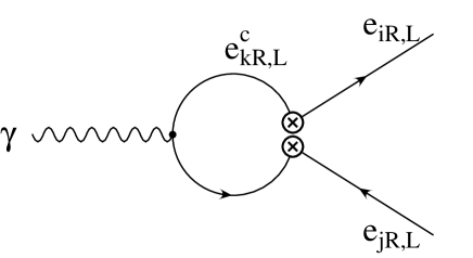
Figure 1: The one-loop contribution to the electromagnetic current in the effective theory.

To show the power of the effective lagrangian description of new physics we compute the form factors starting from the lagrangian (1). The one loop diagram giving rise to $\mu$–$e$ conversion is depicted in fig. 1. By using the $\overline{\mathrm{MS}}$ renormalization scheme and choosing the renormalization scale, $\mu=\Lambda$, where $\Lambda$ is the scale of new physics, we find for the form factors:

$$f_{E0}= \frac{-q^{2}}{(4\pi)^{2}2\Lambda^{2}}\bigg{[}\frac{4}{3}\left(\alpha^{LL}_{ke;k\mu}+\,\alpha^{RR}_{ke;k\mu}\right) \bigg{(}\ln\frac{-q^{2}}{\Lambda^{2}}+F(r_{k})\bigg{)}$$ (17)

$$+\left(\alpha^{L}_{e\mu}+\,\alpha^{R}_{e\mu}\right)\bigg{]}\,,$$

$$f_{M0}= \frac{-q^{2}}{(4\pi)^{2}2\Lambda^{2}}\bigg{[}\frac{4}{3}\left(\alpha^{LL}_{ke;k\mu}-\,\alpha^{RR}_{ke;k\mu}\right) \bigg{(}\ln\frac{-q^{2}}{\Lambda^{2}}+F(r_{k})\bigg{)}$$ (18)

$$+\left(\alpha^{L}_{e\mu}-\,\alpha^{R}_{e\mu}\right)\bigg{]}\,,$$

$$f_{M1}= \frac{m^{2}_{\mu}}{(4\pi)^{2}\Lambda^{2}}\left(\alpha^{\sigma L}_{e\mu}+\,\alpha^{\sigma R}_{e\mu}\right)\,,$$ (19)

$$f_{E1}= \frac{m^{2}_{\mu}}{(4\pi)^{2}\Lambda^{2}}\left(\alpha^{\sigma L}_{e\mu}-\,\alpha^{\sigma R}_{e\mu}\right)\,,$$ (20)

where $r_{k}=m^{2}_{k}/(-q^{2})$, with $m_{k}$ being the masses of the fermions running in the loop, and

$$F(r)=\ln r+4r-\frac{5}{3}+(1-2r)\sqrt{1+4r}\,\ln\left(\frac{\sqrt{1+4r}+1}{\sqrt{1+4r}-1}\right)\,.$$ (21)

There are three important limiting cases. If $r\to 0$ (i.e., $k=e$) then $F(r)=-5/3,$ if $r\approx 1$ (i.e., $k=\mu$) then $F(r)\approx 0.18$ and if $r\gg 1$ (i.e., $k=\tau$) then $F(r)=\ln r.$ The loop diagram in fig. 1 give contributions only to the form factors $f_{E0}$ and $f_{M0}$ but not to $f_{E1}$ and $f_{M1}.$ Because of the UV divergence find in the loop calculation those contributions always contain a term which is proportional to $\ln(q^{2}/\Lambda^{2})$ or $\ln(m_{\tau}^{2}/\Lambda^{2}).$ This term which is completely independent of the details of the model that originate the four-fermion interaction gives a large enhancement for the form factors $f_{E0}$ and $f_{M0}$ while the enhancement is absent in the form factors $f_{E1}$ and $f_{M1}$. Consequently, the $\mu$–$e$ conversion is enhanced while $\mu\rightarrow e\ \gamma$ is not. In this class of models, in which $\mu$–$e$ conversion is dominated by this large logarithmic term one can neglect all the non-logarithmic contributions which are the ones that depend on the details of the complete theory.

4 An explicit model

Let us consider for a moment an extension of the SM by adding just a doubly charged scalar singlet $\kappa^{++}$. Its coupling to right-handed leptons are described by

$${\cal L}_{\kappa}=h_{ij}\overline{e_{iR}^{c}}e_{jR}\,\kappa^{++}+\mathrm{h.c.}$$ (22)

Here the Yukawa coupling matrix $h_{ij}$ is symmetric in the generation indices $i,j$. From this interaction we obtain easily, see fig. 2, the four-fermion interaction

$$\frac{1}{m_{\kappa}^{2}}h^{*}_{ki}h_{lj}(\overline{e_{iR}}e_{kR}^{c})(\overline{e_{lR}^{c}}e_{jR})\,.$$ (23)

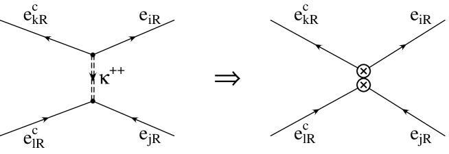
Figure 2: Tree-level matching.

This interaction is of the type ${\cal L}^{RR}$. Comparing with eq. (7) one can immediately identify

$$\alpha_{ik;lj}^{RR}=h^{*}_{ik}h_{lj}\hskip 28.45274pt{\mathrm{and}}\hskip 28.45274pt\Lambda=m_{\kappa}\,.$$ (24)

On the other hand, by using the techniques in [15] one can easily obtain the contributions from matching to the full theory at one loop to the rest of the $\alpha$’s. The one loop diagrams involving $\kappa^{++}$ are depicted in fig. 3.

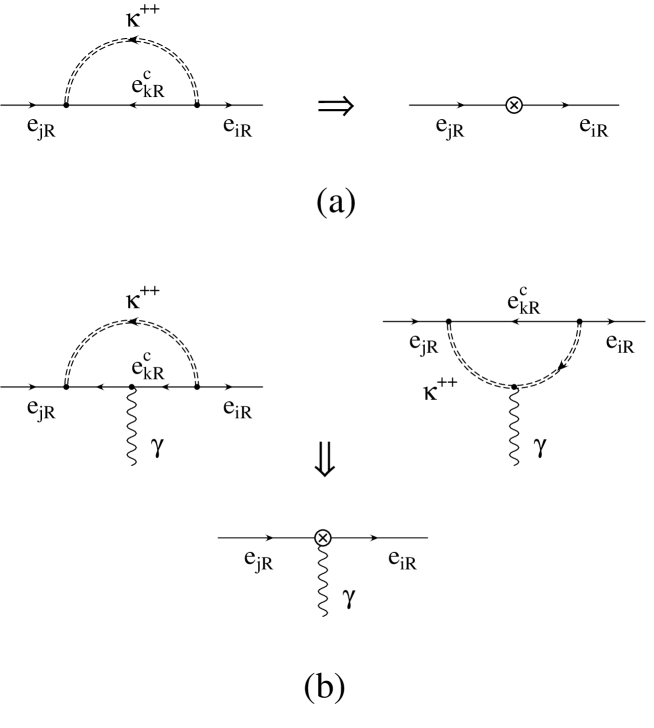
Figure 3: One-loop matching.

Those diagrams are computed by using dimensional regularization and, after subtraction of the effective theory contributions, fig. 1, they can be expanded in $1/m^{2}_{\kappa}$. We keep at most terms of order $1/m^{2}_{\kappa}$. At this order there are contributions to the self-energies and to the vertex of the photon. Those give three types of operators: charge radius operators, eq. (2) and eq. (3), magnetic moment operators, eq. (4) and eq. (5), and operators that involve three covariant derivatives of the fermions. The last operators can be removed by using the equations of motion in favour of mass terms and do not lead to any interesting physics. Therefore, after wave function renormalization, in order to write the kinetic terms in canonical form, the only operators generated in this model are those appearing in the lagrangian (1), but only the right-handed components. By using the $\overline{\mathrm{MS}}$ renormalization scheme and by choosing the renormalization scale $\mu=\Lambda=m_{\kappa}$, we obtain the following coefficients

$$\alpha_{ij}^{R} = \frac{20\,h^{*}_{ki}h_{kj}}{9},$$ (25)

$$\alpha_{ij}^{\sigma R} = \frac{2\,h^{*}_{ki}h_{kl}}{3}\,.$$ (26)

Adding up the contributions from these operators and the contributions coming from the diagram in fig. 1, i.e., substituting eqs. (25), (26) in eqs. (17)–(20), we obtain exactly the same amplitudes as obtained from a calculation in the full model up to terms ${\cal O}((m_{\mu}/m_{\kappa})^{4})$. Therefore the full amplitude for $\mu$–$e$ conversion is dominated by the divergent contribution from the diagram in fig. 1. In the effective field theory language one says that the amplitude is dominated by the running from the scale of new physics $\Lambda=m_{\kappa}$ to relevant scale of the process: in the case of $\mu$–$e$ conversion, $m_{\mu}$ (or $m_{\tau}$ if $\tau$ leptons are running in the loop). This conclusion is independent on the model as long as four-fermion interactions eq. (6) and/or eq. (7) exist.

As expected, in this model there are no contributions to $\overline{e_{R}}\gamma_{\mu}e_{R}Z^{\mu}$ since the physics of a scalar singlet decouples for $m_{\kappa}\gg\Lambda_{F}$. This means that the contributions of the scalar can only lead to operators suppressed by, at least, $1/m_{\kappa}^{2}$. For instance one could easily obtain an operator like eq. (3) with the photon replaced by the $Z$-boson. The contribution of those operators to $\mu$–$e$ conversion, however, are suppressed by a factor $(m_{\mu}/m_{Z})^{2}$ with respect to the photonic contributions.

5 Numerical results and conclusions

Now we are ready to compare the branching ratios of $\mu$–$e$ conversion and $\mu\rightarrow e\ \gamma$ in the class of models we consider and to analyze the relative potential of different experiments to test muon flavour conservation. For definiteness we consider only the right-handed operators in lagrangian (1). We first study the general case in the framework of our effective theory and then we apply the results to our specific model. Substituting the form factors (17)-(20) to eq. (14) and taking only the dominant logarithmic terms (with $\Lambda=1$ TeV in the logarithms) we find

$$R^{Ti}_{\mu e} = 1.2\;(0.5)\cdot 10^{-5}\;\mbox{\rm TeV}^{4}\;\left(\frac{\alpha_{ke;k\mu}^{RR}}{\Lambda^{2}}\right)^{2}\,,$$ (27)

$$R^{Pb,\,Au}_{\mu e} = 3.5\;(1.4)\cdot 10^{-5}\;\mbox{\rm TeV}^{4}\;\left(\frac{\alpha_{ke;k\mu}^{RR}}{\Lambda^{2}}\right)^{2}\,,$$ (28)

where the first number in the expressions corresponds to $k=e,\;\mu$ and the number in the brackets to $k=\tau$. If $k=\tau$ the logarithm enhancement is $\ln(m_{\tau}/\Lambda)$ instead of $\ln(m_{\mu}/\Lambda)$ and it is slightly smaller than in the $\mu$ or $e$ cases. Note that the conversion is somewhat enhanced in $Pb$ and $Au$ (in fact, maximized [25]) if compared with $Ti$.

In the effective lagrangian framework $\mu\rightarrow e\ \gamma$ does not get contributions from loops in fig. 1 and, therefore, it is not enhanced by large logarithms. In any full theory in which both $\mu$–$e$ conversion and $\mu\rightarrow e\ \gamma$ are induced by loops all the couplings should be of the same magnitude (compare, e.g., eq. (24) with eq. (26) in our doubly charged scalar model). Assuming $\alpha^{\sigma R}\equiv\alpha^{RR}$ we obtain

$$R_{\gamma}=1.2\cdot 10^{-5}\;\mbox{\rm TeV}^{4}\;\left(\frac{\alpha_{ke;k\mu}^{RR}}{\Lambda^{2}}\right)^{2}\,$$ (29)

for any type of fermion in the loop.

Comparison of eqs. (27), (28) with eq. (29) shows that due to the presence of large logarithms the $\mu$–$e$ conversion rate is comparable or even exceeds the $\mu\rightarrow e\ \gamma$ rate. To constrain new physics we have to also take into account the sensitivity of experiments. The present experimental upper limits on the branching ratios of the processes are $R^{Ti}_{\mu e}(exp)\mathrel{\vbox{\hbox{$<$}\nointerlineskip\hbox{$\sim$}}}4.3\cdot 10^{-12}$ [1], $R^{Pb}_{\mu e}(exp)\mathrel{\vbox{\hbox{$<$}\nointerlineskip\hbox{$\sim$}}}4.6\cdot 10^{-11}$ [2] and $R_{\gamma}(exp)\mathrel{\vbox{\hbox{$<$}\nointerlineskip\hbox{$\sim$}}}4.9\cdot 10^{-11}$ [31]. SINDRUM II experiment at PSI taking presently data on gold will reach the sensitivity $R^{Au,\,expected}_{\mu e}\mathrel{\vbox{\hbox{$<$}\nointerlineskip\hbox{$\sim$}}}5\cdot 10^{-13}$ [30] and starting next year the final run on $Ti$ it should reach $R^{Ti,\,expected}_{\mu e}\mathrel{\vbox{\hbox{$<$}\nointerlineskip\hbox{$\sim$}}}3\cdot 10^{-14}$ [4]. Normalizing the branching ratios to the experimental upper limits we get for $\Lambda=1$ TeV

$$\frac{R^{Ti}_{\mu e}}{4.3\cdot 10^{-12}} = 11.4\;(5.7)\;B^{Ti}\,\frac{R_{\gamma}}{4.9\cdot 10^{-11}}\,,$$ (30)

$$\frac{R^{Pb,\,Au}_{\mu e}}{4.6\cdot 10^{-11}} = 3.1\;(1.25)\;B^{Au}\,\frac{R_{\gamma}}{4.9\cdot 10^{-11}}\,,$$ (31)

where, again, numbers in the brackets correspond to the case $k=\tau$ and the factors $B,$ $B=R_{\mu e}^{present}(exp)/R_{\mu e}^{future}(exp),$ take into account the improvements in the experimental sensitivity. Eq. (30) and eq. (31) constitute the central result of this work: in the class of models we consider searches for $\mu$–$e$ conversion in both $Ti$ and $Pb$ constrain new physics more stringently than searches for $\mu\rightarrow e\ \gamma$. In addition, from SINDRUM II one expects to achieve $B^{Au}=92.$ already in forthcoming months and $B^{Ti}=1.4\cdot 10^{2}$ next year. If the aimed sensitivity will be achieved then $\mu$–$e$ experiments probe the couplings $\alpha$ of new physics more than one order of magnitude more stringently than $\mu\rightarrow e\gamma.$

$R=$	$4.6\cdot 10^{-11}$	$4.3\cdot 10^{-12}$	$5.0\cdot 10^{-13}$	$3.0\cdot 10^{-14}$
log-enhanced $\mu$–$e$	32	44	101	158
non-enhanced $\mu$–$e$	7	9	20	32
$\mu\rightarrow e\gamma$	23	41	70	141

Table 1: Values of $\Lambda$, in TeV, probed in $\mu$–$e$ conversion and $\mu\rightarrow e\ \gamma$ for different upper bounds on the branching ratios. The upperbound $4.6\cdot 10^{-11}$ is the present bound for $\mu$–$e$ conversion on $Pb$ and it is very close to the present $\mu\rightarrow e\ \gamma$ bound ($4.9\cdot 10^{-11}$). $4.3\cdot 10^{-12}$ is the present bound for $\mu$–$e$ conversion on $Ti$. $5\cdot 10^{-13}$ and $3\cdot 10^{-14}$ are the expected bounds in the next year for $\mu$–$e$ conversion on $Au$ and $Ti$, respectively.

To show which scales of new physics $\Lambda$ can be probed in $\mu$–$e$ conversion and $\mu\rightarrow e\ \gamma$ experiments we have presented the values of $\Lambda$ in TeV-s in Table 1 for different experimental upper bounds on the branching ratios of the processes. All the couplings $\alpha$ are taken to be equal to unity. We have considered both classes of models with and without logarithmic enhancement of $\mu$–$e$ conversion. If the experimental limits for $\mu$–$e$ conversion and $\mu\rightarrow e\ \gamma$ are equal then $\mu$–$e$ conversion enhanced by large logarithms has better sensitivity to $\Lambda$ than $\mu\rightarrow e\ \gamma$, especially in the case of $Pb$ and $Au$ experiments. The scales testable reach $\Lambda\sim{\cal O}(10^{2})$ TeV. However, $\mu$–$e$ conversion without logarithmic enhancement can only probe scales lower by about a factor 5.

To illustrate the discussion above let us present the experimental bounds on the couplings $h$ of $\kappa^{++}$ in our model. Substituting the couplings in eqs. (24)-(26) to eqs. (17)-(20) and using the present experimental limit for $Ti$ we obtain from $\mu$–$e$ conversion for $m_{\kappa}=1$ TeV

$$h_{e\mu}h_{ee}^{*}\;,\;h_{\mu\mu}h_{e\mu}^{*}\; \mathrel{\vbox{\hbox{$<$}\nointerlineskip\hbox{$\sim$}}} \;\frac{6\cdot 10^{-4}}{\sqrt{B^{Ti}}}\,,$$

$$h_{\tau\mu}h_{e\tau}^{*}\; \mathrel{\vbox{\hbox{$<$}\nointerlineskip\hbox{$\sim$}}} \;\frac{9\cdot 10^{-4}}{\sqrt{B^{Ti}}}\,,$$ (32)

while $\mu\rightarrow e\gamma$ gives

$$h_{k\mu}h_{ek}^{*}\; \mathrel{\vbox{\hbox{$<$}\nointerlineskip\hbox{$\sim$}}} \;3\cdot 10^{-3}\,.$$ (33)

The bounds (32) are new limits on the off-diagonal doubly charged scalar interactions (note that tree level $\mu\rightarrow 3e$ probes only $h_{\mu e}h_{ee}^{*}$). While derived for the right-handed singlet the limits apply with a good accuracy also for the interactions of triplet scalars appearing in models with enlarged Higgs sectors as well as in left-right symmetric models This is because the doubly charged component of triplet gives the dominant contribution both to $\mu$–$e$ conversion and $\mu\rightarrow e\ \gamma$. Note that the upper bounds (32) are going to be improved by an order of magnitude with new $\mu$–$e$ conversion data.

Finally, we would like to stress that our main result, the logarithmic enhancement of $\mu$–$e$ conversion rate, is completely general and applies to all models with effective interactions of four charged fermions. For simplicity we have constrained ourselves to purely leptonic operators. However, the same effect is also present for operators involving quarks. To get large logarithms one just needs light charged fermions in the loop. Therefore, loop induced $\mu$–$e$ conversion is also enhanced in models with broken $R$-parity [32] and leptoquarks but not in $R$-conserving MSSM or SUSY GUT’s considered in ref. [7] in which the light fermions in loops are necessarily neutral.

In conclusion, using the effective lagrangian description of new physics we have pointed out a wide class of models with effective four charged fermion interactions in which loop induced $\mu$–$e$ conversion in nuclei is enhanced by large logarithms. With the present upper limits on $\mu$–$e$ conversion and $\mu\rightarrow e\gamma$ branching ratios bounds on new physics (occurring at loop level) derived from these processes are more restrictive in the case of $\mu$–$e$ conversion. In nearest future this factor will increase by more than one order of magnitude due to the expected improvements in sensitivity of already running $\mu$–$e$ conversion experiments. This general result is confirmed by exact calculations in the extension of the SM with doubly charged singlet scalar.

References

- [1] SINDRUM II Collaboration, C. Dohmen et al., Phys. Lett. B317 (1993) 631.
- [2] SINDRUM II Collaboration, W. Honecker et al., Phys. Rev. Lett. 76 (1996) 200.
- [3] S. Ahmad et al., Phys. Rev. D38 (1988) 2102.
- [4] A. van der Schaaf (spokesman of SINDRUM II), PSI proposal R-87-03, 1987.
- [5] M. Bachman et al., BNL Proposal P940, 1997; for a review see also, A. Czarnecki, hep-ph/9710425.
- [6] For original references see, e.g., J.D. Vergados, Phys. Rep. 133 (1986) 1; S.M. Bilenky and S.T. Petcov, Rev. Mod. Phys. 59 (1987) 671.
- [7] See, e.g., R. Barbieri and L. Hall, Phys. Lett. B338 (1994) 212; R. Barbieri, L. Hall and A. Strumia, Nucl. Phys. B445 (1995) 219; T.S. Kosmas and J.D. Vergados, Phys. Rep. 264 (1996) 251, and references therein.
- [8] W.J. Marciano and A.I. Sanda, Phys. Rev. Lett. 38 (1977) 1512; G. Altarelli et al., Nucl. Phys. B125 (1977) 285.
- [9] T.P. Cheng, L. Li, Phys. Rev. D22 (1980) 2860; G.B. Gelmini, M. Roncadelli, Phys. Lett. B99 (1981) 411; H.M. Georgi, S. Glashow and S. Nussinov, Nucl. Phys. B193 (1981) 297.
- [10] J.C. Pati, A. Salam, Phys. Rev. D10 (1974) 275; R.N. Mohapatra, J.C. Pati, Phys. Rev. D11 (1975) 566, ibid. 2558; G. Senjanovic, R.N. Mohapatra, Phys. Rev. D12 (1975) 1502; R.N. Mohapatra, G. Senjanovic, Phys. Rev. Lett. 44 (1980) 912; R.N. Mohapatra, G. Senjanovic, Phys. Rev. D23 (1981) 165.
- [11] C.S. Aulakh and R.N. Mohapatra, Phys. Lett. B119(1982) 136; L.J. Hall and M. Suzuki, Nucl. Phys. B231 (1984) 419; J. Ellis et al., Phys. Lett. B150 (1985) 142; G.G. Ross and J.W.F. Valle, Phys. Lett. B151 (1985) 375; S. Dawson, Nucl. Phys. B261 (1985) 297; R. Barbieri and A. Masiero, Nucl. Phys. B267 (1986) 679.
- [12] W. Buchmüller, R. Rückl and D. Wyler, Phys. Lett. B191 (1987) 442.
- [13] J. Bernabéu, A. Pich and A. Santamaria, Phys. Lett. 148B (1984) 229.
- [14] A. Zee, Phys. Lett. 93B (1980) 389; S.T. Petcov, Phys. Lett. 115B (1982) 401.
- [15] M. Bilenky and A. Santamaria, Nucl. Phys. B420 (1994) 47.
- [16] K. Babu, Phys. Lett. B203 (1988) 132.
- [17] See for instance, H. Georgi, Nucl. Phys. B361 (1991) 339; H. Simma, Z. Phys. C61 (1994) 67; C. Arzt, Phys. Lett. B342 (1995) 189.
- [18] D. Ng and J.N. Ng, Phys. Lett. B320 (1994) 181; Phys. Lett. B331 (1994) 371.
- [19] J. Bernabéu, A. Pich and A. Santamaria, Phys. Lett. 200B (1988) 569; Nucl. Phys. B363 (1991) 326. For an effective lagrangian calculation of radiate corrections to see S. Peris and A. Santamaria, Nucl. Phys. B445 (1995) 252.
- [20] D. Ng and J.N. Ng, Phys. Lett. B331 (1994) 371; D. Tommasini et al., Nucl. Phys. B444 (1995) 451; G. Barenboim and M. Raidal, Nucl. Phys. B484 (1997) 63.
- [21] S.M. Bilenky, S.T. Petcov and B. Pontecorvo, Phys. Lett. 67B (1977) 309.
- [22] J. Bernabeu, E. Nardi and D. Tommasini, Nucl. Phys. B409 (1993) 69.
- [23] S. Weinberg and G. Feinberg, Phys. Rev. Lett. 3 (1959) 111.
- [24] T.S. Kosmas and J.D. Vergados, Nucl. Phys. A510 (1990) 641.
- [25] H.C. Chiang et al., Nucl. Phys. A559 (1993) 526.
- [26] T.S. Kosmas, Amand Faessler and J.D. Vergados, nucl-th/9704020.
- [27] J.E. Kim, P. Ko and D.-G. Lee, Phys. Rev. D56 (1997) 100.
- [28] S. Davidson, D. Bailey and B. Campell, Z. Phys. C61 (1994) 613.
- [29] H.C. Chiang, E. Oset and P. Fernandez de Cordoba, Nucl. Phys. A510 (1990) 591.
- [30] A. van der Schaaf (spokesman of SINDRUM II), private communication.
- [31] R.M. Barnett et al., Review of Particle Physics, Phys. Rev. D54 (1996) 1.
- [32] K. Huitu, J. Maalampi, M. Raidal and A. Santamaria, FTUV/97-45, to appear elsewhere.