Oscillations of moments and structure of multiplicity distributions in $e^{+}e^{-}$ annihilation

Abstract

Starting from the recognized fact that oscillations of moments with rank and shoulder structure in the multiplicity distribution have the same origin in the full sample of events in $e^{+}e^{-}$ annihilation, we push our investigation to the 2-jet sample level, and argue in favor of the use of the negative binomial multiplicity distribution as the building block of multiparticle production in $e^{+}e^{-}$ annihilation events. It will be shown that this approach leads to definite predictions for the correlation structure, e.g., that correlations are flavour independent.

1 FRAMEWORK AND DEFINITIONS

This work is a step in the direction of the description of multiplicity distributions (MD’s) and correlations functions within a common framework: this is the approach we chose in order to investigate the dynamical mechanism of multiparticle production. In particular, in this work we explore the relationship between the multiplicity distribution, $P_{n}$, i.e., the probability of producing $n$ charged final particles, and the $q$-particle correlation function $C_{q}(y_{1},\dots,y_{q})$, using $e^{+}e^{-}$ annihilation data.

We will use the following moments of the MD:

a)  the factorial moments:

$$F_{q}=\sum_{n=q}^{\infty}n(n-1)\cdots(n-q+1)P_{n}$$ (1)

b)  the factorial cumulant moments:

$$K_{q}=F_{q}-\sum_{i=1}^{q-1}\binom{q-1}{i}K_{q-i}F_{i}$$ (2)

c)  their ratio $H_{q}$:

$$H_{q}=\frac{K_{q}}{F_{q}}$$ (3)

and will study these moments as a function of the order $q$ (see [1] for more details). While the above definitions are valid in any restricted region of phase space, the work reported here refers only to full phase space.

It should be noticed that the following relation holds:

$$K_{q}=\int dy_{1}\dots dy_{q}C_{q}(y_{1},\dots,y_{q})$$ (4)

where the integration is over the full phase space, and $C_{q}(y_{1},\dots,y_{q})$ is the correlation function obtained from the inclusive $m$-particle densities ($m=1,\dots,q$) by cluster expansion [2].

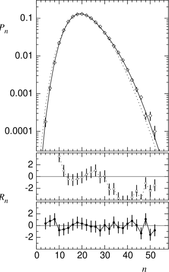
Figure 1: Final charged particles MD for the full sample of events at $\sqrt{s}=91$ GeV from the Delphi Collaboration (diamonds) and fits with eq. 7 (dotted line, open circles in the residuals) and 9 (solid line, filled circles in the residuals).

Figure 2: $H_{q}$ ratio from the MD’s in figure 1

The discussion in the following sections is based on a detailed analysis of published experimental data. A few points should be made clear in advance:

a)  Because of charge conservation, the number of particles in full phase space must be even, so all MD’s in the following must be understood as ‘in their even component only’, e.g.,

$$P_{n}=P_{n}^{\text{(NBD)}}(\mu,k)$$ (5)

should be read as

$$P_{n}\propto\begin{cases}P_{n}^{\text{(NBD)}}(\mu,k)&\text{if $n$ is even}\\ 0&\text{if $n$ is odd}\end{cases}$$ (6)

where a proportionality constant serves the purpose of normalization. This procedure is normally used in the literature [2].

b)  Because the experimental data sample is finite, the tail of the distribution cannot be fully sampled, and the published MD’s are indeed truncated at some value; all analytical MD’s in the following are understood to be truncated at the same value as the corresponding experimental ones. The importance of truncation on the analysis of the ratio $H_{q}$ is well known and has been investigated in [3].

c)  Fits performed on the published MD’s suffer from the fact that the matrix used to go from the measured MD to the reconstructed MD in the unfolding procedure (see, e.g., [4]) is not usually published. Thus a correct, unbiased regression cannot be made; the fits we describe here should then be seen more as ‘solid predictions’ rather than ‘solid results’. As predictions, they are indeed quite intriguing and our approach should therefore be considered as a strong suggestion to the experimental groups.

d)  For the same reason discussed in c), the error bars we plot here for the ratio $H_{q}$ should be considered indicative: the method of varying randomly each $P_{n}$ within its standard error with a Gaussian distribution many times in order to calculate the variance of the $H_{q}$ should be applied to the uncorrelated $P_{n}$ (i.e., before unfolding); however, even if we apply it to published data, it agrees with experimental results [5].

2 THE FULL SAMPLE OF EVENTS

We begin by examining the full sample of events at $\sqrt{s}=91$ GeV. Data on MD’s have been published by all Collaborations, but in order to be consistent and concise we will only use the data published by the Delphi Collaboration [4] (reference [5] contains a more detailed analysis). In [4], the negative binomial distribution (NBD) is fitted to the data; it is worth recalling the explicit expression for the NBD:

$$P_{n}^{\text{(NBD)}}(\mu,k)=\\ \frac{k(k+1)\cdots(k+n-1)}{n!}\frac{\mu^{n}k^{k}}{(\mu+k)^{n+k}}$$ (7)

where the two parameters $\mu$ and $k$ are related to the first two moments as

$$\mu=\langle n\rangle\quad\text{and}\quad k^{-1}=K_{2}/\mu^{2}$$ (8)

The description of the data by the NBD is clearly unsatisfactory from the point of view of the chi-square (see table 1a), and also from the point of view of the residuals (shown in figure 1 with open dots): there is a clear structure which relates to what has been called ‘shoulder structure’ in $P_{n}$ [6]. The corresponding situation with the ratio $H_{q}$ is shown in figure 2, from which it is evident that a single truncated NBD (dotted line) cannot describe the oscillations of $H_{q}$ with $q$.

It was shown by the Delphi Collaboration [6] that the shoulder structure can be explained in terms of the superposition of the MD’s resulting from classifying the events according to the number of jets, and that the MD in each class is well fitted by a NBD. Moreover, the goodness of this description is not influenced by varying the parameter of the jet-finding algorithm.

It is then natural to try a description of the full sample of events with the weighted sum of two NBD’s [5], one corresponding to 2-jet events and the other to 3-jet events (4-jet events’ contribution is negligible). This is implemented by forcing the weight to be equal to the fraction of 2-jet events as experimentally measured in [6]. The resulting MD is thus

$$P_{n}=\alpha_{\text{2-jet}}P_{n}^{\text{(NBD)}}(\mu_{\text{2-jet}},k_{\text{2-jet}})+\\ (1-\alpha_{\text{2-jet}})P_{n}^{\text{(NBD)}}(\mu_{\text{3-jet}},k_{\text{3-jet}})$$ (9)

This fit is shown with a solid line in figure 1 for $\alpha_{\text{2-jet}}=0.767$, corresponding to $y_{\text{min}}=0.06$ in the jet-finder JADE; the parameters of the fit are shown in table 1b. In the same figure we also notice that the structure of the residuals has greatly improved, and in figure 2 that the $H_{q}$ ratio is also well described (solid line). Furthermore, the parameters we find from our fit are consistent with those obtained experimentally fitting the 2- and 3-jet samples separately with single NBD’s. Analogous result can also be obtained analyzing the SLD and OPAL data [5]; L3 data [7] are consistent with SLD’s.

Table 1: Parameters of the MD’s fitted to the data as shown in the figures. Part a) refers to figure 1 (dotted line); part b) to figure 1 (solid line); part c) to figure 3 (dotted line); part d) to figure 3 (solid line).

a)	$\mu$	$21.4\pm 0.9$
	$k$	$24.3\pm 0.7$
	$\chi^{2}$/NDF	80/34
b)	$\mu_{\text{2-jet}}$	$19.4\pm 0.2$
	$k_{\text{2-jet}}$	$52\pm 6$
	$\mu_{\text{3-jet}}$	$27.3\pm 0.3$
	$k_{\text{3-jet}}$	$\kern 5.00002pt61\pm 10$
	$\chi^{2}$/NDF	12/21
c)	$\mu$	$18.5\pm 0.1$
	$k$	$57\pm 3$
	$\chi^{2}$/NDF	20/16
d)	$\mu_{\text{light}}$	$17.2\pm 0.2\kern 5.00002pt$
	$\mu_{\text{heavy}}$	$22.0\pm 1.6\kern 5.00002pt$
	$k$	$145\pm 53\kern 5.00002pt$
	$\chi^{2}$/NDF	13/16

3 THE 2-JET SAMPLE OF EVENTS

It is a striking result, and a lesson to be learned from the analysis mentioned in the previous section, that one can resolve puzzling structures by investigating them on a deeper level. It is a prediction of the same analysis that the 2-jet sample should be well described (in all its aspects) by one NBD. However, this turns out not to be entirely true, as shown in figure 3, which reproduces the 2-jet data and (single) NBD fit by Delphi [6]. While the chi-square is satisfactory (see table 1c), the residuals (open dots in the figure) show some structure, although much less pronounced than in the full sample; the ratio $H_{q}$ (figure 4) still shows oscillations, albeit an order of magnitude less deep than in the previous case.

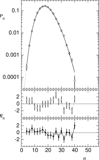
Figure 3: Final charged particles MD for the 2-jet sample of events ($y_{\text{min}}=0.02$) at $\sqrt{s}=91$ GeV from the Delphi Collaboration (diamonds) and fits with eq. 7 (dotted line, open circles in the residuals) and 10 (solid line, filled circles in the residuals).

Figure 4: $H_{q}$ ratio from the MD’s in figure 3

A few results coming from experiments will help us investigate deeply the structure of 2-jet events. First, the result by OPAL [8] on forward–backward correlations: they are weak, and in the bulk they are explained by the superposition of events with a fixed number of jets; the residual correlation is attributed to the presence of events with quarks of heavy flavour. This suggests that longitudinal observables can reveal the flavour structure of the original hard event. Second, the result by Delphi on the MD in one hemisphere [9]: a sample enriched in $b\bar{b}$ events was found to be essentially identical in shape to the MD of the full sample, apart from a shift of one unit. If taken literally, and if forward–backward correlations are neglected except for the requirement of even total charged multiplicity, this result suggests that the $b\bar{b}$ events MD, when the fraction of $b\bar{b}$ events is small, is very similar to the light $q\bar{q}$ MD, except for a translation of two units.

Guided by all the above considerations, we propose to use a NBD to describe the MD of a 2-jet event of fixed flavour. We identify two types of hadronic events: those originating from a $b\bar{b}$ pair and those from a $q\bar{q}$ pair, where with $q$ we indicate all flavours lighter than $b$. We thus use for the MD of 2-jet events the weighted sum of two NBD’s:

$$P_{n}=\alpha_{\text{heavy}}P_{n}^{\text{(NBD)}}(\mu_{\text{heavy}},k)+\\ (1-\alpha_{\text{heavy}})P_{n}^{\text{(NBD)}}(\mu_{\text{light}},k)$$ (10)

Here $\alpha_{\text{heavy}}=0.22$ is the experimentally determined fraction of $b\bar{b}$ decays of the $Z^{0}$ at $\sqrt{s}=91$ GeV. The subscripts ‘heavy’ and ‘light’ refer respectively to $b\bar{b}$ and $q\bar{q}$ events. It should be noticed that the parameter $k$ is the same in both NBD’s, while the difference between the average values is not fixed. This reflects the above considerations on single hemisphere multiplicity.

The description of published data by the above parameterization is very good, as shown in table 1d and in figures 3 and 4 (solid lines and solid dots), from all points of view: chi-square, residuals and $H_{q}$ analysis. It is further supported by the fact that a few simpler alternatives do not work as well [10].

4 SUMMARY AND CONCLUSIONS

A relatively simple parameterization, based on phenomenological considerations and previous experimental analyses and results, has been shown to describe very well the charged particle multiplicity distribution in $e^{+}e^{-}$ annihilation at LEP energy, including the tail, that is the moments of high order. This is so even at the very specific level of the 2-jet sample of events.

This parameterization is characterized by the presence of two types of events (heavy and light quarks decays of the $Z^{0}$) and by the fact that each of these is described by a negative binomial distribution. Since for 2-jet events each hemisphere correspond to one jet, and the two hemisphere are practically uncorrelated, we conclude that the MD of a “single quark-jet” is described by the NBD. Thus we are lead to suggest that the NBD is the fundamental building block of multiparticle production in $e^{+}e^{-}$ annihilation.

Finally, it was shown that the single quark-jet NBD has a parameter $k$ which is the same for all flavours. Because of the relation between $k$ and $K_{2}$, eq. 8 above, we conclude that true correlations are expected to be flavour independent.

It should be stressed that all mentioned conclusions are predictions which can easily be the subject of experimental testing; we think indeed that the results of these tests will improve our understanding of multiparticle dynamics and of the properties of strong interactions.

References

- [1] R. Ugoccioni, in Proceedings of the XXVI International Symposium on Multiparticle Dynamics (Faro, Portugal, 1996) ed.s J. Dias de Deus et al.: World Scientific, Singapore, 1997, p. 208.
- [2] E.A. De Wolf, I.M. Dremin and W. Kittel, Physics Reports 270 (1996) 1.
- [3] R. Ugoccioni, A. Giovannini and S. Lupia, Phys. Lett. B 342 (1995) 387.
- [4] P. Abreu et al., DELPHI Collaboration, Z. Phys. C 52 (1991) 271.
- [5] A. Giovannini, S. Lupia and R. Ugoccioni, Phys. Lett. B 374 (1996) 231.
- [6] P. Abreu et al., DELPHI Collaboration, Z. Phys. C 56 (1992) 63.
- [7] W. Kittel, these Proceedings.
- [8] R. Akers et al., OPAL Collaboration, Phys. Lett. B 320 (1994) 417.
- [9] P. Abreu et al., DELPHI Collaboration, Phys. Lett. B 347 (1995) 447.
- [10] A. Giovannini, S. Lupia and R. Ugoccioni, Phys. Lett. B 388 (1996) 639.