Diffractive Exclusive Photon Production in DIS at HERA
Abstract
We demonstrate that perturbative QCD allows one to calculate the absolute
cross section of diffractive exclusive production of photons
at large at HERA, while the aligned jet model allows one to estimate
the cross section for intermediate .
Furthermore, we find that the imaginary part of the amplitude for the
production of real photons is larger than the imaginary part of the
corresponding DIS amplitude by about a factor of , leading to the
prediction of a significant
counting rate for the current generation of experiments at HERA. We also find
a large azimuthal angle asymmetry
in scattering for
HERA kinematics which allows one to directly measure the real part of the
DVCS amplitude and hence the nondiagonal parton distributions.
PACS: 12.38.Bx, 13.85.Fb, 13.85.Ni.
Keywords: Hard Diffractive Scattering, Deeply Virtual Compton Scattering,
Nondiagonal Parton Distributions.
I Introduction
Recent data from HERA has spurred great interest in exclusive or diffractive direct production of photons in scattering (DVCS- deeply virtual Compton scattering) as another source to obtain more information about the gluon distribution inside the proton for nonforward scattering. In recent years studies of diffractive vector meson production and deeply virtual Compton scattering has greatly increased our theoretical understanding about the gluon distribution in nonforward kinematics and how it compares to the gluon distribution in the forward direction. For a less than complete list of recent references see Ref. [1, 2, 3, 4, 5, 6, 7, 8, 9, 10, 11].
Exclusive diffractive virtual Compton processes at large , first investigated in [12], offer a new and comparatively “clean”[13] way of obtaining information about the gluons inside the proton in a nonforward kinematic situation. We are interested in the production of a real photon compared to the inclusive DIS cross section. The exclusive process is nonforward in its nature, since the photon initiating the process is virtual () and the final state photon is real, forcing a small but finite momentum transfer to the target proton i.e forcing a nonforward kinematic situation as we would like. We will show that pQCD can be applied to this type of exclusive process although we will not give a formal proof on the level comparable to the DIS case [14]. Such a proof can be found in Ref. [15].
The paper is organized in the following way. In Sec. II we estimate the amplitude in the normalization point using the aligned jet model approximation and conclude that for such the nondiagonal amplitude is larger than the diagonal one by a factor of . In Sec. III we calculate the imaginary part of the amplitude for in the leading order of the running coupling constant and compare it to the imaginary part of the amplitude in DIS in the same order. In Sec. IV we argue that at sufficiently small the -dependence of the cross section should reflect the interplay of hard and soft physics typical of diffractive phenomena in DIS. Namely, that at fixed and increasing , hard physics should tend to occupy the dominant part of the space of rapidities. In contrast to this, at fixed and decreasing , hard physics should occupy a finite range of rapidities which increases with - with at the HERA energy range due to the QCD evolution, and that soft QCD physics occupies the rest of the phase space. In Sec. V we give the total cross section of exclusive photon production and give numerical estimates of the DVCS production rate at HERA and find that such measurements are feasible for the current generation of experiments. We also show the feasibilty of directly measuring the real part of the DVCS amplitude and hence, at least, the shape of the nondiagonal parton distributions through a large azimuthal angle asymmetry in scattering for HERA kinematics. Sec. VII finally contains concluding remarks.
II The amplitude for diffractive virtual Compton scattering at intermediate
Similar to the case of deep inelastic scattering, in real photon production it is possible to calculate within perturbative QCD the evolution of the amplitude but not its value at the normalization point at few GeV2 where it is given by nonperturbative effects. Hence we start by discussing expectations for this region. It was demonstrated in [17] that the aligned jet model [16] coupled with the idea of color screening provides a reasonable semiquantitative description of . In this model the virtual photon interacts at intermediate and small via transitions to a pair with small transverse momenta - () and average masses which thus carry asymmetric fractions of the virtual photon’s longitudinal momentum. Due to large transverse color separation, , the aligned jet model components of the photon wave function interact strongly with the target with the cross section . Neglecting contributions of the components of the wave function with smaller color separation, one can write using the Gribov dispersion representation [18] as [17]:
| (1) |
where the factor in the nominator is due to the overall phase volume, . The factor is the fraction of the whole phase volume occupied by the aligned jet model , and the factor is due to the propagators of the photon in the hadronic intermediate state with mass2 equal . Based on the logic of local quark-hadron duality (see e.g.[19] and references therein) we take the lower limit of integration . In the case of real photon production the imaginary part of the amplitude for is
| (2) |
with being the flux factor. The only difference from Eq. 1 for is the change of one of the propagators from to - here is the energy of the virtual photon in the rest frame of the target.
Approximating as a constant for the range in question (we understand this in the sense of a local duality of the hadron spectrum and the loop) we find
| (3) |
In the following analysis we will take for the perturbative QCD evolution as 2.6 GeV2 to avoid ambiguities. It is easy convince oneself that for and Eq.3 leads to . A similar value of has been obtained within the generalized vector dominance model [20] As we will see below QCD evolution leads to a strong increase of with increase of for fixed . However it does not change appreciably the value of .
III The amplitude for exclusive real photon production at large .
The process of exclusive direct production of photons in first nontrivial order of at small can be calculated (see Fig. 1) as the sum of a hard contribution calculated within the framework of QCD evolution equations [25] and a soft contribution which we evaluated above within the aligned jet model. The hard contribution can be described through a two gluon exchange of a box diagram with the target proton. In order to calculate the imaginary part of the amplitude, we need to calculate the hard amplitude from the box as well as the gluon-nucleon scattering plus the soft aligned jet model contribution. Let us first give a general expression for the imaginary part of the amplitude and then proceed to deal with the gluon-nucleon scattering, followed by the calculation of the box diagrams.

First, let us discuss the hard contribution which actually dominates in the considered process. To account for the gluon-nucleon scattering, we work with Sudakov variables for the gluons with momenta and attaching the box to the target and the following kinematics for the gluon-nucleon scattering:
| (4) |
where and are light-like momenta related to the momenta of the target proton and the probing virtual photon respectively, by:
| (5) | |||
| (6) |
with being the Bjorken and the proton momentum fraction carried by the outgoing gluon. Equivalent equations to Eq. 4 apply for with the only difference being that is replaced by , the momentum fraction of the incoming gluon, signaling that there is only a difference in the longitudinal momenta but not in the transverse momenta. This fact will shortly become important. Furthermore there is a simple relationship between and : following from the kinematics of the considered reaction[21] where is the asymmetry parameter or skewedness of the process under consideration. Therefore one is left with just the integration over since cannot vary independently of . Being exclusively interested in the small region, one can safely make the following approximations: and . Since we are working in the leading approximation, neglecting corrections of order , the main contribution comes from the region , hence the contribution to the imaginary part of the amplitude simplifies considerably. First, since , one has and the polarization tensor of the propagator of the exchanged gluon in the light-cone gauge becomes, see Ref. [18] :
| (7) |
In other words it is enough to take the longitudinal polarizations of the exchanged gluons into account.
Using Eq. 7 one obtains the following expression for the total contribution of the box diagram and its permutations:
| (8) |
where is the sum of the box diagrams, is the amplitude for the gluon-nucleon scattering, a,b are the color indices and the overall tensor structure has been neglected for now. The usage of the imaginary part of the scattering amplitude and in particular limiting ourselves to the s-channel contribution as the dominant part in both the forward and the nonforward case (Eq. 8) is correct (see Ref. [5] for more details) as long as we restrict ourselves to the DGLAP region of small and thus small , where is the square of the momentum transfered to the target. The real part of the amplitude will be evaluated below by applying a dispersion relation over the center of mass energy . Using Eq. 7 and the Ward identity which is the same as in the Abelian case since the box contains no gluons i.e is color neutral:
| (9) |
yielding
| (10) |
one can rewrite Eq. 8 as:
| (11) |
where we have used (the average over the transverse gluon polarization) and defined the imaginary part of the hard scattering to be given by:
| (12) |
where the sum over repeated indices is implied. Up to this point we have just rewritten the equation for the imaginary part of the total amplitude but have not identified the different perturbative and non-perturbative pieces. In the case of a virtual photon with longitudinal polarization, this would be an easy task since the pair would only have a small space-time separation and we could follow the argument in Ref. [1, 4, 19] stating that the box is entirely dominated by the hard scale and thus can unambiguously be calculated in pQCD. However, in our case we are dealing with a virtual photon which is transversely polarized and thus one can have large transverse space separations between and . The resolution to this problem can be found in the following way: one accepts that one has a contribution from a soft, aligned-jet-model-type, configuration and that there is no unambiguous separation of the amplitude in a perturbative and non-perturbative part up to a certain scale . However, in the integration over transverse gluon momenta, one will reach a scale at which a clear separation into perturbative and non-perturbative part can be made and hence we can unambiguously calculate albeit not the imaginary part of the amplitude of the upper box but its derivative i.e its kernel convoluted with a parton distribution. At this point then, one can include the non-perturbative contribution of the aligned jet model into the initial distribution of the imaginary part of the total amplitude and solve the differential equation in . One obtains the following solution for the imaginary part [25]:
| (13) |
where is the evolution kernel[26] and starting from the gluon distribution can be defined from Feynman diagrams in the leading approximation by realizing that in Eq. 11 one can replace and by and one finds:
| (14) |
where is the nondiagonal parton distribution in general. Comparison of Eq. 11 with the QCD-improved parton model expression for the total cross section of charm production given in [24] shows that in the case is the conventional, diagonal gluon distribution.
Note that the parton distribution which serves as an input in Eq. 13 has to be evolved over the -range covered by the integral which complicates the calculation. We will explain below how to deal with this issue in practical situations.
At this point we would like to comment on equivalent definitions of nondiagonal parton distributions in the literature which differ by kinematic factors (see for example [4, 6, 7]). Eq. 14 corresponds to the definition used in [7], however since it is given on the level of Feynman diagrams there are no ambiguities such as renormalization of bilocal operators and hence it provides an unambiguous definition of a nondiagonal parton distribution.
For the non-perturbative input, we will be able to use the aligned jet model analysis of Sec. II and the standard relation between and :
| (15) |
Following the discussion above, we now only need to calculate to leading logarithmic accuracy, in order to make predictions for the imaginary part of the whole amplitude. Therefore, let us now consider the box diagram where the two horizontal quark propagators are cut, corresponding to the DGLAP region i.e neglecting the u-channel contribution.

The kinematics (see Fig. 2) for the calculation of the cut box diagram, using Sudakov variables, is the following. The quark-loop momentum is given by:
| (16) |
where and are light-like momenta related to by:
| (17) | |||
| (18) |
The momenta of the exchanged gluons, in light cone coordinates, are given by:
| (19) |
where we have assumed the transverse momentum of the proton to be zero. The probing transverse photon and the produced photon have the following momenta, again in light cone coordinates:
| (20) |
is calculated in the light cone gauge yielding the following result for the most general case[27]:
| (21) |
The DIS kernel is analogous to Eq. 21 except that and the kernel for real photon production is obtained for .
We now can proceed to calculate the total imaginary part of the amplitude from Eq. 13 where we parameterize the gluon distribution at small as:
| (22) |
We neglect the dependence for the moment[28]. The above parameterization is taken from CTEQ3L as well as the parameterization of in terms of in leading order:
| (24) | |||||
| (26) | |||||
with , and given by:
| (27) |
where we have taken and .
The ratio of the imaginary parts of the amplitudes[29] is given by:
| (28) |
We give in the range from to and for a of and since this kinematic range is relevant at HERA. One might ask what about the contributions due to quarks. The answer is that the corrections are small[30] but for completeness we include them here. Eq. 13 is then augumented with a similar expression for the quark contribution where the kernel is now that of quark-quark splitting and the nondiagonal parton distribution is that of the quark:
| (30) | |||||
where the general expression for the kernel, after a similar calculation as before, is found to be:
| (31) |
and the + - prescription is the one used in Ref. [5]. The quark distribution itself is also taken from CTEQ3L[31] and given by:
| (32) |
with
| (34) | |||||
| (35) |
We chose to be constant since it varies only between and in the range of interest, i.e. the error we make is almost negligible since the quark distribution themselves are small in the -range considered. Furthermore, according to our discussion in Sec. II, we chose the initial distribution for the imaginary part of the DVCS amplitude to be twice that of the initial distribution for the imaginary part of the DIS amplitude. In the evolved QCD part, the nonforward kinamtics are taken into account in the kernels of the QCD evolution equation, also the different evolution of nondiagonal as compared to diagonal distribution has been taken into account as explained below.
As the calculation with MATHEMATICA showed, the amplitude of the production of real photons is larger than the DIS amplitude over the whole range of small and turns out to be between , and for , , and for and , and for in the given range. It has to be pointed out that for a given , the ratio is basically constant. Of course, the ratio will approach as is decreased to the nonperturbative scale since this is our aligned jet model estimate The reason for the deviation from is due to the difference in the evolution kernels.
It is worth noting that in the kinematics we discuss, the ratio is still rather sensitive to the nonperturbative boundary condition. For example, assuming the same boundary conditions for DVCS and DIS, would result in a reduction of of about at and
In Eq. 13 the median point of the integral corresponds to . This is due to the mass of the in the quark loop being . For such a the ratio of nondiagonal and diagonal gluon densities weakly depends on . Hence with an accuracy of a few percent we can approximate this ratio by its value at . Therefore, in the calculation of , we used Eq. 22 and 32 for both the diagonal and nondiagonal case but then multiplied the real photon result of the amplitude by a function for each and to take into account the different evolution of the nondiagonal distribution as compared to the diagonal one,
| (36) |
The function was determined by using our modified version of the CTEQ-package and, starting from the same initial distribution and evolving the diagonal and nondiagonal distribution to a certain . We then0 compared the two distributions at the value for different and then interpolated for the different ratios of the distribution in for given . For this median point the difference between the diagonal and nondiagonal gluon distribution is between depending on the and involved and for the quarks (see the figures in Ref. [5, 11] for more details).
As far as the complete amplitude at small is concerned, we can reconstruct the real part via dispersion relations [22, 23], which to a very good approximation gives:
| (37) |
Meaning that since can be fitted as , is independent of to a good precision. Therefore, our claims for the imaginary part of the amplitude also hold for the whole amplitude at small . This is due to the fact that within the dispersion representation of the amplitude over the contribution of the subtraction constant becomes negligible at sufficiently small .
One also has to note that there is a potential pitfall since the QED bremsstrahlung - the Bethe-Heitler process, where the electron interacts with a proton via a soft Coulomb photon exchange and the real photon is radiated off the electron, can be a considerable background. As was shown by Ji [6], the Bethe-Heitler process will give a strong background at small and medium and . We will discuss this subject in more detail later on.
IV The t-slope of the cross section
The slope of the differential cross section of the virtual Compton scattering is determined by three effects: (i) the average transverse size of the component of the and wave functions involved in the transition, (ii) the pomeron-nucleon form factor in the nucleon vertex, and (iii) Gribov diffusion in the soft part of the ladder. This leads to several qualitative phenomena. In the normalization point, configurations of an average transverse size, comparable to that of the -meson, give the dominant contribution to the scattering amplitude, leading to a slope similar to that of the processes . The contribution of the higher mass components is known to result in an enhancement of the differential cross section of the Compton scattering at by a factor as compared to the prediction of the vector meson dominance model with intermediate states, see e.g. [32]. Since the diffraction of a photon to masses has a smaller slope than for transitions to and , one could expect that the high mass contribution would lead to a t-slope of the Compton cross section being somewhat smaller than for the production of -mesons. However direct experimental comparison [32] of the slopes of the Compton scattering and the -meson photoproduction at finds these slopes to be the same within the experimental errors. Using these data, we can estimate the slope of the amplitude for diffractive photon production in DIS at HERA energies but at moderate Q-i.e. in the normalization point as
| (38) |
where , , and [33]. Hence for HERA energies .
In another limit of large and large enough , say , the dominant configurations have small a transverse size and the upper vertex does not contribute to the slope. Furthermore, the perturbative contribution occupies most of the rapidity interval and leaves no phase space for the soft Gribov diffusion. In this case, the slope is given by the square of the two-gluon form factor of the nucleon which corresponds to [1, 2].
An interesting situation emerges in the limit of large but fixed when the energy starts to increase. In this case, the perturbative part of the ladder has the length . Here , where is the fraction of the parent parton at a soft scale. For HERA kinematics for and increasing with increasing . This is consistent with the observation of an approximate factorization for diffraction in the case of high masses (, ) in the scattering of real and virtual photons observed at HERA [34], namely
| (39) |
The observed slope for these processes is which is consistent with the presence of a cone shrinkage at the rate as compared to the data at lower energies where smaller values of were probed. Similarly we can expect that for virtual Compton scattering at large , the slope will increase with decrease of , at very small , approximately as
| (40) |
where . We take into account here that was determined experimentally from the processes at .
V The rate of exclusive photon production at HERA
To check the feasibility of measuring a DVCS signal against the DIS background, we will be interested in the fractional number of DIS events to diffractive exclusive photoproduction events at HERA in DIS given by:
| (41) |
with
| (42) |
from applying the optical theorem and where is the ratio of the amplitudes given by Eq. 28, and is given by Eq. 37, with . Note, that even though we used the total DVCS cross section in Eq. 41 we only need the ratio of the imaginary parts of the amplitudes to calculate . A complete expression for DVCS will be given in the next section. Note that only is calculable in QCD. The dependence is taken from data fits to hard diffractive processes.
Using the fact that one can rewrite Eq. 41:
| (43) |
where for the given range. We computed , the fractional number of events given by Eq. 43, for between and and for a of and where the numbers for were taken from [35]. Based on our analysis of the previous section we use Eq. 38 for , assuming that for the slope drops by about 1 2 units as compared to Eq. 38 to account for the decrease of the transverse size of the -pair; for larger we use Eq. 39.
We find at and ; at and ; at and ; and finally at and . As is to be expected, the number of events rises at small since the differential cross section is proportional to the square of the gluon distribution and the total cross section is just proportional to the gluon distribution i.e. the ratio in Eq. 41 is expected to be proportional to the gluon distribution and this assumption is born out by our calculation and falls with increasing since does not grow as fast with energy.
VI The complete cross section of exclusive photon production
In order to study whether the Bethe-Heitler or DVCS Process will be dominant in real photon production we need the expressions for the differential cross sections first.
We find that the differential cross section for DVCS can be simply expressed through the DIS differential cross section by multiplying the DIS differential cross section by (see Eq. 43) which was calculated in the previous section. One can see this by observing how is related to as given in Sec. V and to via in the same section. We then find using Eq. 43 for
| (44) |
with using the same exponential dependence as in the previous section and being the ratio of the imaginary parts of the DIS to DVCS amplitudes as computed earlier.
In writing Eq. 44 we neglected - the experimentally observed conservation of s channel helicities justifies this approximation - and assumed . where ist the energy of the electron in the final state and , where is the azimuthal angle between the plane defined by and the final state proton and the plane and is the azimuthal angle between the plane defined by the initial and final state electron and the plane (see Fig. 3).

In case of the Bethe-Heitler process, we find the differential cross section at small to be
| (45) |
with , being the invariant energy and the fraction of the scattered electron/positron energy. and are the electric and nucleon form factors and we describe them using the dipole fit
| (46) |
where is the proton magnetic moment. We make the standard assumption that the spin flip term is small in the strong amplitude for small .
In order to write down the complete total cross section of exclusive photon production we need the interference term between DVCS and Bethe-Heitler. Note that in the case of the interference term one does not have a spinflip in the Bethe-Heitler amplitude, i.e. , one only has , as compared to Eq. 45 containing a spinflip part, i.e. , . The appropriate combination of and which yields is
| (47) |
We then find for the interference term of the differential cross section, where we already use Eq. 45,
| (49) | |||||
with the + sign corresponding to electron scattering off a proton and the - sign corresponding to the positron. The total cross section is then just the sum of Eq. 44,45 and 49.
A t-dependence of Bethe-Heitler as compared to DVCS for different
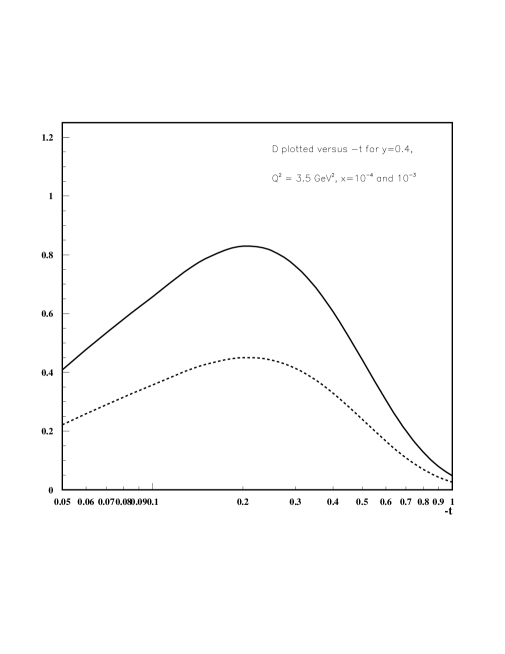
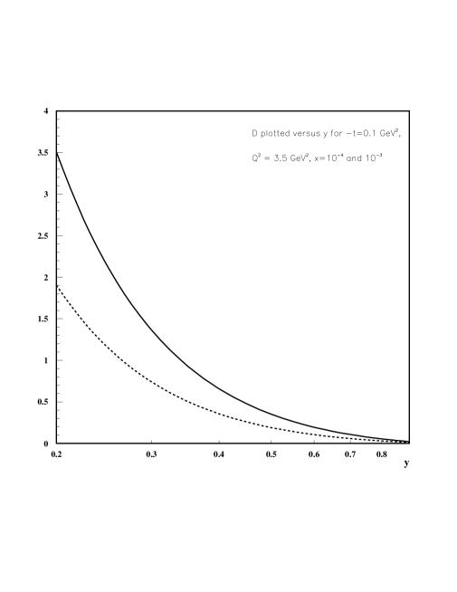
At this point it is important to determine how large the Bethe-Heitler background is as compared to DVCS for HERA kinematics, hence, in the following discussion, we will estimate the ratio allowing a background comparison:
| (50) |
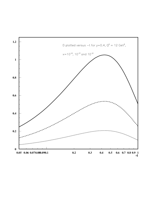
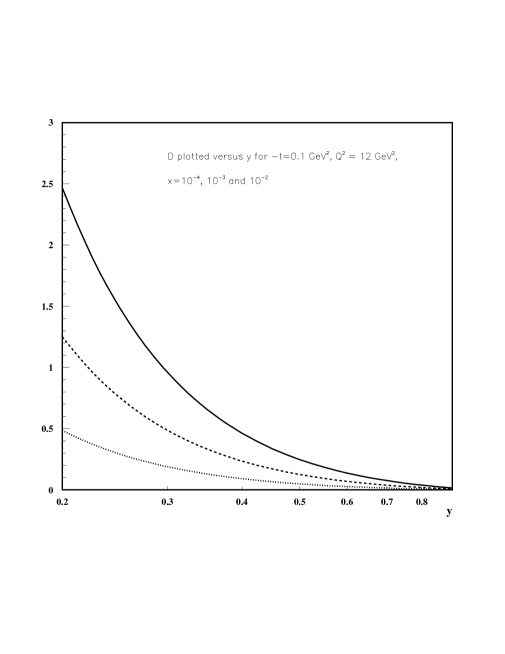
with . Using the expressions from Sec. VI, we compute and find [see Figs. 4a and 6a] for relatively small and with the given values of and considered. Note, however, that this does not mean that the case for DVCS is hopeless. As it turns out, it is rather advantageous to have when looking at the interference term which we will do next. Also note that there is a very strong energy dependence of which extends the range where DVCS is significantly larger than Bethe-Heitler with increasing energy.
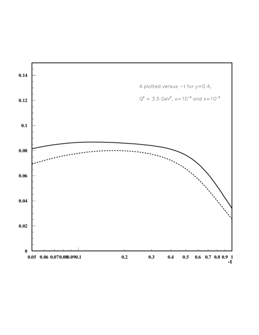
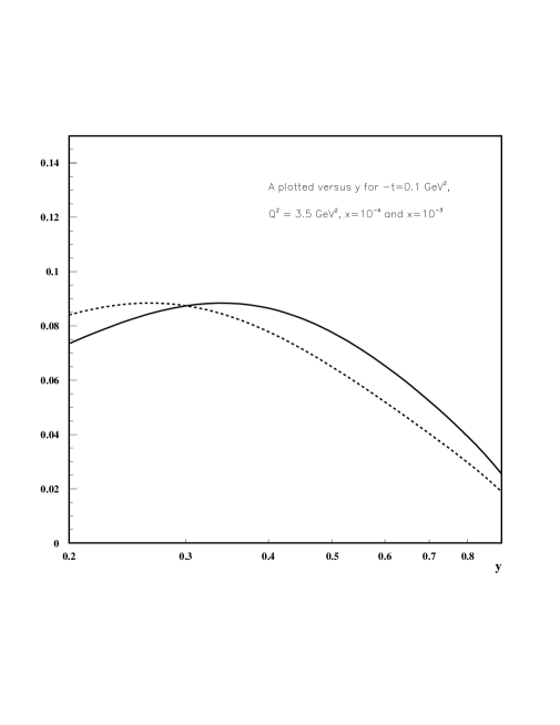
It is convenient to illustrate the magnitude of the intereference term in the total cross section by considering the asymmetry for proton and either electron or positron to be in the same and opposite hemispheres ( we omit the rather cumbersome explicit expression but the reader can easily deduce it from Eq. 44,45 and 49. )
| (51) |
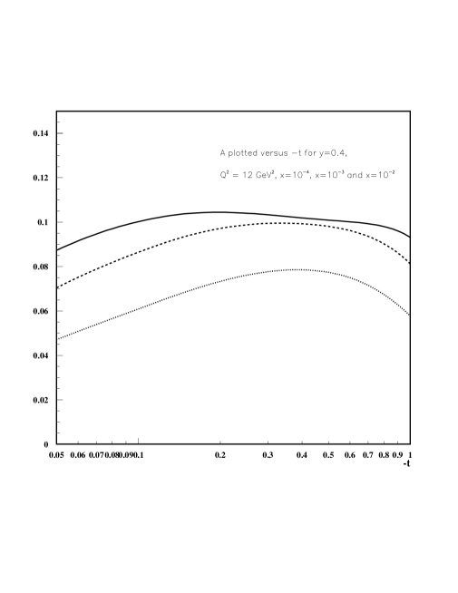
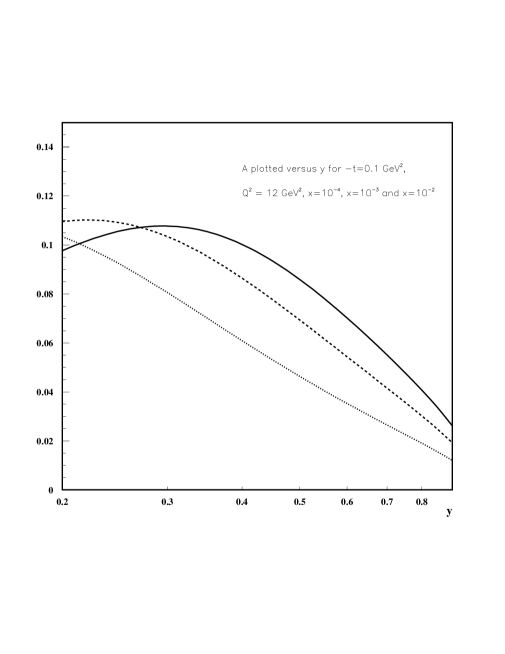
in other words, one is counting the number of events in the upper hemisphere of the detector minus the number of events in the lower half, normalized to the total cross section. Fig. 5a,b and 7a,b show for the same kinematics as above and we find that the asymmetry is fairly sizeable already for small and is strongly dependent on the energy. Due to this fairly large asymmetry, one has a first chance to access nondiagonal parton distributions through this asymmetry. We will discuss in more detail, in particular its energy dependence, in an upcoming paper.
Note, there is an increased experimental difficulty to measure DVCS if the recoil proton is not detected in other words if is not directly measured. However there is a simple, practical way around this problem which we will discuss next.
B DVCS alternative to tagged proton in the final state
Another interesting process, which can be studied in the context of DVCS, is the one where the nucleon dissociates into mass “X” - . Perturbative QCD is applicable in this case as well. In particular the following factorization relation should be valid at sufficiently large :
| (52) |
The big advantage of the dissociation process as compared to the process where the target proton stays intact is that the Bethe-Heitler process is strongly suppressed for inelastic diffraction at small t due to the conservation of the electro-magnetic current, hence the amplitude is multiplied by an additional factor which is basically for the Bethe-Heitler process. Thus, the masking of the strong amplitude of photoproduction is small in this case. Since there is already data available on production, this quantity can give us information on how different the slopes for the production of massless to massive vector particles are, providing us with more understanding on how different or similar the exact production mechanisms are. Note that the ratio of the total dissociative to elastic cross section of meson production is found to be about at large [36] which is basically of . The same should hold true for production and in fact this ratio should be a universal quantity. This is due to the fact that one has complete factorization, hence the hard part plus vector meson is essentially a point and thus for the soft part, is does not matter what kind of vector particle is produced. The above said implies for Eq. 52 that it also should be of order unity, implying that the order of magnitude of the fractional number of events for real photon production to DIS remains unchanged even though the actual number of might decrease by as much as .
VII Conclusions
In the above said we have shown that pQCD is applicable to exclusive photoproduction by showing that the ratio of the imaginary parts of the amplitudes of DIS to a real photon is calculable in pQCD after specifying initial conditions since the derivative in energy of the hard scattering amplitudes can be unambiguously calculated in pQCD and all the non-perturbative physics can then be absorbed into a parton distribution. We wrote down an evolution equation for the imaginary part of the amplitude, which can be generalized to the complete amplitude at small , and solved for the imaginary part of the amplitude. We also found that the imaginary part of the amplitude of the production of a real photon is larger than the one in the case of DIS in a broad range of for the reasons as discussed above. We also found the same to be true for the full amplitude at small . We also make experimentally testable predictions for the number of real photon events and suggest that the number of events are small but not too small such that after improving the statistics on existing or soon to be taken data, it would be feasible to access the nondiagonal gluon distribution at small from this clean process. Finally, we demonstrated that measuring the asymmetry at HERA, which is fairly sizable in the kinematics in question, would allow one to determine the real part of the DVCS amplitude, in other words gain a first experimental insight into nondiagonal parton distributions, despite .
Acknowledgments
We thank A.Mueller who back in 1995 drew our attention to the importance of this process. We would like to thank A.V. Radyushkin for critical comments on an earlier draft of this paper and R. Engel who drew our attention to the fact that H1 data indicate an independence of of the ratio of inclusive high mass hadron production to the total cross section of real and virtual photons. This work was supported by the Department of Energy under grant number DE-FG02-93ER40771.
REFERENCES
- [1] S.J. Brodsky, L.L. Frankfurt, J.F. Gunion, A.H. Mueller, and M. Strikman, Phys. Rev. D50 (1994) 3134; see also [2]
- [2] L.L. Frankfurt, W. Koepf, and M. Strikman, Phys. Rev. D54 (1996) 3194.
- [3] A. Radyushkin Phys. Lett. B385 (1996) 333.
- [4] J.C. Collins, L. Frankfurt, and M. Strikman, Phys. Rev. D56 (1997) 2982.
- [5] L.L. Frankfurt, A. Freund, V. Guzey and M. Strikman, Phys. Lett. B 418, 345 (1998).
- [6] X.-D. Ji, Phys. Rev. D55 (1997) 7114. .
- [7] A. Radyushkin, hep-ph/9704207, A. Radyushkin, Phys.Lett B380 (1996) 417 and private communication.
- [8] I.I Balitsky and V.M. Braun, Nucl. Phys. B311, 541 (1989).
- [9] J. Bluemlein, B. Geyer and D. Robaschik, hep-ph/9705264.
- [10] A.Martin and M.Ryskin, hep-ph/9711371.
- [11] A. Freund, V. Guzey, hep-ph/9801388.
- [12] J. Bartels and M.Loewe, Z.Phys. C12, 263 (1982).
- [13] Clean in the sense that the wave function of a spatially small size configuration within a real photon is better known as compared to the wave functions of vector mesons thereby removing a big theoretical uncertainty in the determination of the gluon distribution.
- [14] J.C. Collins, D. E. Soper, and G. Sterman, in PERTURBATIVE QUANTUM CHROMODYNAMICS, ed .A.Mueller, pp 1-91, World Scientific Publ.,1989.
- [15] J.C. Collins, A. Freund, hep-ph/9801262.
- [16] J. D. Bjorken in Proceedings of the International Symposium on Electron and Photon Interactions at High Energies,p. 281–297, Cornell (1971); J. D. Bjorken and J. B. Kogut, Phys. Rev. D8 (1973) 1341.
- [17] L. L. Frankfurt and M. Strikman, Phys. Rep. 160 (1988) 235; Nucl.Phys. B316(1989) 340.
- [18] V. N. Gribov, Sov. Phys. JETP 30 (1969) 709.
- [19] L. Frankfurt, A. V. Radyushkin, M. Strikman, Phys. Rev. D55 (1997) 98.
- [20] L.Frankfurt, V.Guzey, M.Strikman, hep-ph/9712339.
- [21] In the case of the imaginary part of the amplitude which we discuss at this point, one has and we can treat the soft part as a parton distribution function (the DGLAP regime), whereas if one would have the situation of a distributional amplitude as first discussed by Radyushkin [3] which is governed by the Brodsky-Lepage evolution equations.
- [22] V.N.Gribov and A.A.Migdal, Yad.Fiz. 8 (1968) 1002 Sov.J.Nucl.Phys. 8 (1969) 583.
- [23] J.B.Bronzan, Argonne symposium on the Pomeron, ANL/HEP-7327 (1973) p.33; J.B.Bronzan, G.L.Kane, and U.P.Sukhatme, Phys.Lett. B 49, 272 (1974).
- [24] M.A. Shifman,A.L. Vainshtein and V.I. Zakharov Nucl.Phys.B136,157 (1978), M. Glueck, E. Reya, Phys.Lett. B83, 98 (1979).
- [25] H. Abramowicz, L.L. Frankfurt and M. Strikman, DESY-95-047, SLAC Summer Inst. 1994:539-574.
- [26] In Ref. [7] a similar equation was derived for the complete amplitude for larger , where the quark distribution dominates and one only needs the kernel. Of course, at sufficiently small the contribution of this term is numerically small.
- [27] Note that this expression is defined differently from the gluon quark splitting kernel as given in e.g. Ref. [7] by a factor of due to the fact that the additional already appears in the convolution integral for the derivative.
- [28] This effect will be taken into account in the actual numerical calculation - see discussion below.
-
[29]
The tensor structure which is the same in both cases, namely:
cancels out in the ratio!(53) - [30] We found them to be around in the ratio .
- [31] We used the u-quark parametrization for all light quarks for simplicity, which is surely unprobelamtic at small-.
- [32] A.M.Breakstone et al., Phys.Rev.Lett. 47 (1981) 1778;47 (1981) 1782.
- [33] Note that the data [32] can be equally well described by the fit with and by the fit.
- [34] H1-Collaboration (S.Aid et al.), Phys.Lett. B358 (1995) 412.
- [35] H1-Collaboration (S.Aid et al.), hep-ex/9603004.
- [36] H1-Collaboration (C. Adloff et al.), hep-ex/9705014.