Goldstone Boson Production and Decay

Abstract

Various topics in and around Goldstone Boson Production and Decay in CHPT are discussed, in particular I describe some of the progress in $p^{6}$ Chiral Perturbation Theory Calculations, the progress in calculating hadronic contributions to the muon anomalous magnetic moment, here comparing the two latest results of the light-by-light in some detail. I also present some progress in various $\eta$ and $K$ decays and their relevance for CHPT.

Abstract

Various topics in and around Goldstone Boson Production and Decay in CHPT are discussed, in particular I describe some of the progress in $p^{6}$ Chiral Perturbation Theory Calculations, the progress in calculating hadronic contributions to the muon anomalous magnetic moment, here comparing the two latest results of the light-by-light in some detail. I also present some progress in various $\eta$ and $K$ decays and their relevance for CHPT.

1 Introduction

Most of the other talks at this conference contained a rather well defined topic. This talk was left somewhat undefined and I have therefore taken the liberty of covering topics where there has been a lot of progress since the last Chiral Dynamics Workshop and which were not covered by any of the other plenary talks.

Chiral Dynamics and, espescially, Chiral Perturbation Theory (CHPT) are the main topic in this meeting. It has been introduced by Jürg Gasser ([Gasser]) and the variant relevant for the case of a small quark condensate by Jan Stern ([Stern]). In this talk I will only cover the standard case. See Stern’s talk for references to the nonstandard case.

There is also a large overlap between this talk and the presentation of the working group with the same name ([Bijnens]). I will refer to that talk whenever appropriate. This talk consists of 3 main parts : an overview of the progress in CHPT at order $p^{6}$ in the mesonic sector, a discussion of the relevant chiral dynamics for the hadronic contributions to the muon anomalous magnetic moment and a few selected $K$ and $\eta$ decays.

In section 2 I discuss the presently done full two-loop calculations. In the two flavour, up and down quark, sector there exist quite a few calculations. The $\pi\pi$ scattering amplitude has been discussed both in a plenary talk ([Ecker]) and by several contributions in one of the working groups ([WG2]). I therefore restrict myself to the three other calculations: $\gamma\gamma\to\pi^{+}\pi^{-}$([Burgi]), $\gamma\gamma\to\pi^{0}\pi^{0}$([BGS]) and $\pi\to e\nu\gamma$([BT]). In the three flavour case there exists calculations of the vector and axial-vector two-point functions([GK1, GK2, GK3]) and of a combination of vector form factors corresponding to Sirlin’s theorem([Post]).

Sect. 3 discusses the light-by-light scattering hadronic contribution to the muon anomalous magnetic moment. Here there are two recent calculations, ([HKS3]) and ([BPP2]). I compare the latest numbers of the various sub-contributions in both calculations and their estimated errors. The main remaining differences are in the way errors are included and in the estimate of one contribution where there is a large remaining model dependence.

The next section discusses a few Kaon decays. Here I will concentrate on the decays where chiral dynamics plays a large role. This section is basically a summary of my own and A. Pich’s talk in the meeting on $K$-Physics in Orsay, June 1996 ([Orsay]).

Section 5 concentrates on two $\eta$ decays. $\eta\to\pi\pi\pi$ as a test of chiral dynamics and as input for one quark mass ratio, and $\eta\to\pi^{0}\gamma\gamma$ as a window on high order CHPT contributions.

The last section summarizes the situation as reviewed in this talk.

2 Progress in the Mesonic Sector at order $p^{6}$

2.1 Two-flavour Calculations

2.1.1 $\pi\pi$

As remarked earlier this has been covered by the plenary talk of G. Ecker ([Ecker]) and in more detail by the contributions of Mikko Sainio and Marc Knecht in the $\pi\pi$ and $\pi N$ working group ([WG2]).

2.1.2 $\gamma\gamma\to\pi^{+}\pi^{-}$

The Born term is the same as tree level scattering in Scalar Electro Dynamics and is known since a long time([Brodsky]). Early experiments indicated a large enhancement near threshold over the Born approximation ([PLUTO]). To order $p^{4}$ there is one combination of coupling constants that contributes, $L_{9}+L_{10}$ and there is also a loop contribution([BC]). These do provide an enhancement around threshold but as not as large as ([PLUTO]) indicated. These results were also used to get at the pion polarizabilities as discussed by ([Holstein]). The $p^{6}$ calculations were performed by U. Bürgi ([Burgi]). The number of diagrams is rather large but the final numerical difference is rather small. In Fig. 1 I show the more recent data ([MarkII]) which do not indicate a large threshold enhancement, the Born, $p^{4}$ and $p^{6}$ result. The dotted line is the Born cross-section, the dashed line the $p^{4}$ result and the full line the $p^{6}$ contribution. The data shown are the Mark II data ([MarkII]). The dispersive estimate of Donoghue and Holstein is the dashed-double-dotted line ([DH]).

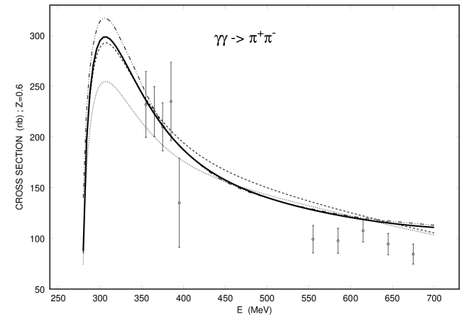
Figure 1: The cross section for $\gamma\gamma\to\pi^{+}\pi^{-}$. Figure taken from (Bürgi 1996).

2.1.3 $\gamma\gamma\to\pi^{0}\pi^{0}$

If we would have used current algebra, we would have gotten a very good “low energy theorem” for this process. The $p^{2}$ contribution obviously vanishes and there is also no contribution at order $p^{4}$, for a modern proof in CHPT see ([BC]). The first contribution would have come from terms like $tr\left(\nabla_{\mu}UF^{L}_{\alpha\beta}\nabla^{\mu}U^{\dagger}F^{R\alpha\beta}\right)$. If we take the naive order of magnitude for the coefficient of this type of terms we would have obtained a cross-section of a few hundredths of a nanobarn. However, in this case it was obvious that the leading contribution would come from charged pion rescattering in the final state. When this process was calculated in CHPT to order $p^{4}$ this was also what was found ([BC, DHL]). The cross-section predicted in this fashion was found to be a few nanobarn. The experimental measurement afterwards ([CB]) obtained a cross section of this order but disagreed in shape and was higher near threshold. This disagreement could be understood in dispersive treatments ([Pennington, DH]).

The calculation at order $p^{6}$ was the first full two-loop calculation in CHPT ([BGS]) and showed the same near threshold enhancement. The result is shown in Fig. 2.

Figure 2: The Crystal Ball data, the $p^{4}$ and the $p^{6}$ CHPT calculation as well as the band from dispersive calculations for $\gamma\gamma\to\pi^{0}\pi^{0}$. Figure taken from (Bellucci 1994).

The reason for the large enhancement near threshold was obvious in the dispersive calculations. At tree level, there is large cancelation between the $I=0$ and $I=2$ amplitudes. The charged pion cross section has a positive interference and the neutral pion cross section vanishes. The two isospin final states have quite different final state interactions which are not too well described by tree level CHPT. This tree level is the contribution in the one-loop result while both the $p^{6}$ result and the dispersive calculations have a larger $I=0$ $\pi\pi$ final state rescattering than the tree level result for it. The final state rescattering thus interferes with the large cancelation present in the neutral pion production, and while both amplitudes have fairly small corrections, as can be seen in the charged pion corrections, the sum can have large corrections.

Both the dispersive calculations and the $p^{6}$ result agree with the Crystal Ball. The physical effect that creates the bending over towards the higher center of mass values is the same in both cases as well. It is the exchange in the $t$-channel of vector mesons. In the CHPT calculation this comes in via the estimate of the $p^{6}$ constants while in the dispersive calculations the vector meson contribution enters via the so-called left-hand cut.

2.1.4 Radiative Pion Decay or $\pi^{+}\to\ell^{+}\nu\gamma$

This process serves as the input process for the combination $L_{9}+L_{10}$ used earlier but it is also interesting in its own right. There are claims that the data cannot be explained by the standard $V-A$ description of semi-leptonic weak decays ([Chizov]). The same data could have been explained by an unusually large momentum dependence of one of the form factors involved in this decay. This decay has three different contributions, there is the inner Bremsstrahlung-component, which is by definition given to all orders in CHPT in terms of the pion decay constant $F_{\pi}$ and there are two structure dependent form factors. The vector form factor is given to lowest order by the anomaly and is known to $p^{6}$ ([ABBC]). Here the $p^{6}$ calculation is only a one-loop calculation. For the pion case there are only small corrections. The axial-vector form-factor has at $p^{4}$ only a tree level contribution ([GL1]), but at two-loop order the loops do contribute ([BT]).

The estimate of the relevant $p^{6}$ constants is given by axial-vector exchange and turns out to be very small in the relevant phase space. Using the standard values of the renormalized couplings at the $\rho$-mass a sizable correction to the $p^{4}$ results is found. The uncertainty due to the uncertainty on the combination $2l_{1}-l_{2}$ is smaller than the uncertainty due to the choice of renormalization scale. The correction is not negligible despite the fact that the leading correction, the terms proportional to $L^{2}=\log^{2}(m_{\pi}/\mu)$ vanish in this case. The size of the various contributions are given in Table 1 for 3 different subtraction points.

Table 1: Some contributions to the axial form factor in $\pi\to e\nu\gamma$ in units of $10^{-2}\cdot GeV^{-1}$.

$\mu$	$m_{\rho}$	0.6 GeV	0.9 GeV
${\cal O}(p^{4})$	$-$5.95	$-$5.95	$-$5.95
$Z_{\pi}$ and $F\to F_{\pi}$	$-$0.22	$-$0.24	$-$0.21
${\cal O}(p^{6})$ 1-vertex of ${\cal L}_{4}$	+1.03	+0.88	+1.19
${\cal O}(p^{6})$ pure two-loop	+0.53	+0.42	+0.59
Total	$-$4.62	$-$4.89	$-$4.44

2.2 Three flavour results

The full list of counterterms has been derived for $N_{f}=3$ by ([FS]) and for general $N_{f}$ by Bijnens, Colangelo and Ecker.

2.2.1 The Vector-Vector two-point function

This has been calculated in ([GK1]) and numerically studied in more detail in ([GK2]). The quantity to be calculated here is

$$\Pi^{V}_{ab}(q^{2})=i\int d^{4}xe^{iq\cdot x}\langle 0|T\left(V_{\mu}^{a}(x)V_{\nu}^{b}(0)\right)|0\rangle\,.$$ (1)

The calculation here is simpler since no “real” two-loop diagram needs to be calculated but the complexity of renormalization at two-loops still hits in its full complexity([GK1]). The spectral function from this calculation is shown in Fig. 3.

More important, this calculation can be used in various sum rules. This leads to predictions for differences of spectral functions in the up,down and strange sector (here in hyper-charge notation):

$$\int_{s_{0}}^{\infty}ds\frac{\rho^{33}_{V}(s)-\rho^{88}_{V}(s)}{s^{n+1}} = (n=0)\Rightarrow Q=(3.7\pm 2.0)~{}10^{-5}$$ (2)

$$= (n\geq 1)\Rightarrow L_{9}^{r}=(6.6\pm 0.3)~{}10^{-3}$$

$$\int_{s_{0}}^{\infty}ds\frac{\rho^{aa}_{V}(s)}{s^{n+2}} = (n=0)\Rightarrow P=-(5.6\pm 0.6)~{}10^{-4}$$ (3)

$$= (n\geq 1)\Rightarrow L_{9}\mbox{ only}$$

The numerical results are taken from ([GK2]). The expressions depend on 4 constants, $L_{9}$ and three combinations of $p^{6}$ constants $P,Q$ and $R$. The two that can be determined via the sum rules agree well with the resonance estimate of the same quantities thus providing evidence that this method for estimating the constants also works at order $p^{6}$. They have recently calculated also the $AA$ two-point function and a similar numerical analysis is under way([GK3]). This is discussed in ([Bijnens]). Other relevant references are the calculation of ([Holdom]) for a two-loop vector two-point function without the renormalization aspects and the calculation by Maltman of the isospin breaking $\langle T(V^{3}V^{8})\rangle$ vector two-point function ([Maltman]).

Figure 3: The vector spectral function at order $p^{4}$ (dashed), $p^{6}$only (dotted) and the sum (full) together with the data from $e^{+}e^{-}$. The buildup of the $\rho$ can be seen here. Figure from (Golowich and Kambor 1995).

2.2.2 Sirlin’s Theorem

In ([Sirlin]) it was proven that the combination

$$\Delta(t)=\underbrace{\frac{1}{2}F^{\pi^{+}}(t)+\frac{1}{2}F^{K^{+}}(t)+F^{K^{0}}(t)}_{\mbox{Electromagnetic\\ Form Factors}}-\underbrace{f_{+}^{K\pi}(t)}_{\mbox{weak $f_{+}$ form-factor}}$$ (4)

only starts at order $(m_{s}-\hat{m})^{2}$. An immediate consequence of this is that at $t=0$ dependence on $p^{6}$ parameters exists, e.g. via terms of the type $\langle u_{\mu}u^{\mu}\chi_{+}^{2}\rangle$. But by powercounting, the $t$-dependence of these form-factors is at most $t(m_{s}-\hat{m})$, and the charge radius of the above combination thus has no contribution from terms in $p^{6}$-Lagrangian. Caution must be taken here, the combination $\Delta(t)$ has large cancelations in it and we can thus expect large higher order corrections. That CHPT is well behaved for this quantity can be seen when comparing the size of the $p^{6}$ correction to the charge radius of $\Delta(t)$ with the individual charge radii of the combination.

The result is ([Post])

$$\langle r^{2}\rangle_{\mbox{Sirlin}} = \left(0.006(p^{4})+0.017(3)(\mbox{reducible})-0.002(\mbox{irr.})\right)~{}fm^{2}$$ (5)

$$= (0.021\pm 0.003)~{}fm^{2}\,.$$

This should be compared with the experimental results

$$\langle r^{2}\rangle_{\mbox{Sirlin}}\hskip-56.9055pt$$ (6)

$$= \left(\frac{1}{2}\left[0.439(8)(\pi^{+})+0.34(5)(K^{+})\right]-0.054(26)(K^{0})-0.36(2)(K\pi)\right)fm^{2}$$

$$= -(0.025\pm.041)~{}fm^{2}\,.$$

The size of the $p^{6}$ correction is less than $10\%$ of the largest terms so it is a nicely converging result. The present experimental precision is too low to significantly test this calculation.

3 Muon Anomalous Magnetic Moment

There is a new experiment on the muon anomalous magnetic moment, $a_{\mu}=(g-2)/2$, planned at BNL ([BNL]). They aim at a precision in $a_{\mu}$ of $4\cdot 10^{-10}$, to be compared with the present precision of $84\cdot 10^{-10}$ from the CERN experiment. The main aim is to unambiguously detect the weak gauge boson loops and put constraints on possible other contributions.

We therefore need to determine the contributions from the strong interaction with great precision. There are three hadronic contributions relevant at the present level of precision, the hadronic vacuum polarization, the higher order vacuum polarization and the light-by-light contribution. The first two depend on the same integral over the hadronic vector spectral function which can be measured in tau decays and in electron-positron collisions. The latest determination is in ([Alemany]) and is also discussed in some detail in ([Bijnens]). Here the main need is for more precise experiments in the rho mass region in order to bring the error down to the precision of the BNL experiment. Theoretical estimates of this quantity are accurate to about 25% ([Rafael, Pallante]).

The light-by-light contribution is more of a problem, it cannot be related to experiments in a simple way and has therefore to be evaluated in a theoretical framework. The relevant quantity is an hadronic four-point function so lattice QCD determinations are probably some time into the future. This quantity has been calculated recently by two groups with the following recent history: (all in units of $10^{-10}$)

$$-3.6\pm 1.6\mbox{(\cite[cite]{[\@@bibref{}{HKS1}{}{}]})};-5.2\pm 1.8\mbox{(\cite[cite]{[\@@bibref{}{HKS2}{}{}]}) and }$$

$$-7.9\pm 1.5\mbox{(\cite[cite]{[\@@bibref{}{HKS3}{}{}]})}$$ (7)

$$-11\pm 5\mbox{(\cite[cite]{[\@@bibref{}{BPP1}{}{}]}) and }-9.2\pm 3.2\mbox{(\cite[cite]{[\@@bibref{}{BPP2}{}{}]}).}$$ (8)

The two results are in fact in quite good agreement with each other on the total value and on the error but they differ in the error combining. The reasons for the change in the numbers are for (7): first a change in the model coupling pseudoscalar mesons (P) to two photons, and for the second change the inclusion of the $\eta^{\prime}$ and a small change with the $P\gamma\gamma$ coupling because of the measured CLEO $P\gamma\gamma^{*}$ form factor. For (8) the change was a change in the $P\gamma\gamma$ coupling to agree better with the preliminary CLEO data (following a suggestion of Kinoshita).

The three different type of contributions to the light-by-light diagram, different in chiral and $N_{c}$ counting are (in units of $10^{-10}$): first (7), second (8)

$\pi^{0}$, $\eta$ and $\eta^{\prime}$ exchange	$-8.3\pm 0.65$	$-8.5\pm 1.3$	Good
axial+scalar exchange	$-0.17$	$-0.93\pm 0.03$
quark loop	$1.0\pm 1.1$	$2.1\pm 0.3$	Good
The ENJL model used for (8) here tends to mix these two contributions,
therefore only the sum can be compared between (7) and (8).
charged pion and Kaon loop	$-0.45\pm 0.81$	$-1.9\pm 1.3$	Main
Model used for loop	HGS	naive VMD	uncertainty
Errors added linearly	$\pm 2.6$	$\pm 3.2$
Errors added quadratically	$\pm 1.5$	$\pm 1.9$

The pseudoscalar exchange contribution we agree on extremely well. The error in ([BPP2]) was chosen larger because we only have tested the models with one photon off-shell, while both photons off-shell contribute also significantly. For the 2nd contribution the error estimate went the other way, in ([HKS2]), there is the freedom of the quark mass, in ([BPP2]) a good matching between long and short distance was observed and hence a smaller error chosen. The main difference is really in the last contribution where two different but equivalently good chiral models were chosen for the relevant $\gamma^{*}\gamma^{*}\pi\pi$ coupling. Both models are chirally invariant and satisfy the correct chiral identities when the off-shellness is extrapolated to the rho-meson pole. In my opinion we should therefore choose the error such that it includes both models.

In conclusion, in order to improve the present situation we need data on the couplings of one and two pseudoscalar mesons to two photons with both photons off-shell.

4 Kaon decays

This section can be found more extensively in the talks by J. Bijnens and A. Pich in ([Orsay]). $CP$-violation and $\varepsilon^{\prime}/\varepsilon$ are also covered in great detail in those proceedings and I will therefore not treat them here. Extensive treatments can also be found in ([DAPHNE]).

4.1 Semi-leptonic Kaon Decays

4.1.1 $K_{l3}$ : $K\to\pi e\nu$, $K\to\pi\mu\nu$

the main problem here is that we need improvement in the experimental situation on the slope of the scalar form factor. It should also be remembered that these decays are our main source of knowledge of the Cabibbo angle, or of $V_{us}$, and thus deserve very accurate measurements.

4.1.2 $K_{l2\gamma}$

this decay is similar to the pion radiative decay discussed above and has similar characteristics. The vector form factor is a test of the anomaly and an accurate measurement of this would be an independent measurement of quark mass effects in anomalous amplitudes. At present the only place where this occurs is in $\eta$ decays and there the question is entangled with $\eta\eta^{\prime}$ mixing. The vector Form factor is known to $p^{6}$([ABBC]) assuming very small direct quark mass effects. The axial vector form factor depends on $L_{9}+L_{10}$ and is thus predicted from the pion decay. Given the corrections seen there at order $p^{6}$ the prediction for this form-factor has an expected error of about 30%.

4.1.3 $K_{l2ll}$

Here again everything is known to order $p^{4}$, there are large enhancement for the modes involving electrons over the inner Bremsstrahlung amplitude and there is good agreement with experiment but the experimental errors are fairly large.

4.1.4 $K_{l4}$

This decay has been discussed in the framework of obtaining new accurate values of the $\pi\pi$ phase shifts. It should not be forgotten that the absolute values of the 4 form-factors are themselves also of interest. They provide additional input for the parameters of CHPT while at the same time providing tests of CHPT ([BCG]). By measuring all the channels one can also test the isospin assumptions underlying the present theory calculations.

4.1.5 $K_{l3\gamma}$

The $p^{4}$ correction is rather small due to a cancelation between the “counterterm” and the loop contributions. This cancelation is in fact necessary to obtain agreement with the measurement of $(3.61\pm 0.014\pm 0.021)\cdot 10^{-3}$ ([Leber]). The tree level, $p^{4}$ prediction is 3.6, 3.8 in the same units([BEG]).

4.2 $K\pi\pi$, $K\to\pi\pi\pi$

This has been discussed extensively by Maiani and Paver in ([DAPHNE]). As was realized in ([DHKW]) the $p^{4}$ calculations leave in fact a series of relations between various slope parameters in $K\to 3\pi$ when the $K\to 2\pi$ and $3\pi$ rates are used as input. These relations provide stringent tests of Chiral Perturbation Theory in this sector and need to be tested so our predictions for CP violating effects can be refined. At present the agreement is satisfactory but especially in the $\Delta I=3/2$ sector the experimental precision is rather poor.

4.3 Rare $K$ decays

This area has been the scene of some of the major successes of CHPT, but there are also some problem cases.

4.3.1 $K_{S}\to\gamma\gamma$

This is a parameter-free CHPT prediction at order $p^{4}$([Kgg]). The experimental measurement of a Branching Ratio of $(2.4\pm 0.9)\times 10^{-6}$ ([Kggexp]) agrees extremely well with the prediction of $2.0\times 10^{-6}$.

4.3.2 $K_{L}\to\gamma\gamma$

This process proceeds through $K_{L}\to\pi^{0},\eta\to\gamma$ and at order $p^{4}$ there is an exact cancelation between these two contributions. As a consequence the predictions is very sensitive to higher order effects and this decay is not really under theoretical control yet.

4.3.3 $K_{L}\to\pi^{0}\gamma\gamma$

This decay is also a parameter-free prediction at order $p^{4}$ ([EPR, CD]). he predicted rate at $p^{4}$ is a branching ratio of $0.67\times 10^{-6}$ to be compared with the measured one of $1.70\times 10^{-6}$ ([Kpgg]). But the phase space distribution is clustered at high $\gamma\gamma$ masses contrary to Vector meson Dominance model predictions and agrees well with the CHPT prediction as shown in Fig. 4.

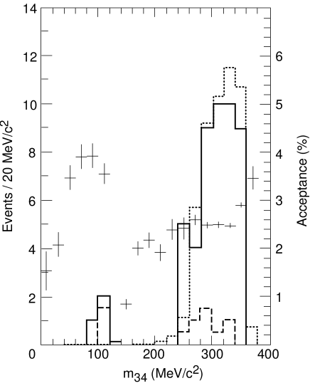
Figure 4: Measured $2\gamma$-invariant mass distribution for $K_{L}\to\pi^{0}\gamma\gamma$ (solid line). The dotted line simulates the $p^{4}$ CHPT prediction, normalized, and the dashed line is the estimated background. The crosses are the experimental acceptance, figure from (Barr 1992).

There are two $p^{6}$ effects expected, unitarity corrections and Vector meson Exchange contributions. The former make the distribution steeper and the latter flatter and they both increase the rate. It is possible to get agreement with both the rate and the spectrum with reasonable estimates of these contributions, see the contribution by A Pich in ([Orsay]) and references therein.

5 $\eta$-decays

5.1 $\eta\to 3\pi$

There are three questions here in the theory :

1. total rates

2. the ratio $\displaystyle r=\frac{\Gamma(\eta\to\pi^{0}\pi^{0}\pi^{0})}{\Gamma(\eta\to\pi^{+}\pi^{-}\pi^{0})}$

3. the Dalitzplot distributions

5.1.1 The Decay Rate

The order $p^{2}$ contribution was calculated a long time ago by Cronin and is about $66~{}eV$. This should be compared with the Particle Data Group width of $280\pm 28~{}eV$. The $p^{4}$ corrections were calculated ([GL2]) and were large, leading to about $167\pm 50~{}eV$. There are two reasons for this large correction: $\eta\eta^{\prime}$ mixing and final state rescattering. The former should be adequately dealt with at the $10\%$ level but the final state corrections could be large. These have been evaluated independently by two groups using dispersive methods ([eta3pi1, eta3pi2]), earlier references can be found in these papers. The $p^{4}$ calculation is used to determine the subtraction constants. The Dalitz plot parameters are used as constraints on the calculation. This leads to a value of $209\pm 20~{}eV$ for the decay width. So, with a slightly large value of $(m_{d}-m_{u})/(m_{s}-\hat{m})$ we reproduce nicely the observed decay rate. This slightly larger value of that quark mass ration was in fact expected from calculated large deviations from Dashen’s theorem ([DHW, Bijnens(1993)]) and a large number of more recent references. One can now turn in fact the argument around and the decay rate of $\eta\to 3\pi$ has become the most accurate source of information on that quark mass ratio. Electromagnetic corrections to the decay rate have since been found to be small as expected from current algebra arguments ([Baur1996]) and ([Gosdzinsky1996]).

5.1.2 $r$

The lowest order prediction for the ratio $r$ is $1.53$, the $p^{4}$ prediction $1.43$ and the dispersive calculations lead to $1.41\pm 0.03$. The Particle Data Group quotes $1.36\pm 0.05$. More precise measurements of this quantity as an important check on the dispersive calculations are therefore welcome.

5.1.3 Dalitzplot

The Dalitzplot is parametrized as $1+ay+by^{2}+cx^{2}$ for the charged decay and as $1+g(x^{2}+y^{2})$ for the neutral decay. The next-to-leading order prediction ([GL2]) and the dispersive results together with the available experimental results are given in Table 2. The last line are new results to be published but cited in ([Amsler]). As is obvious from the table the agreement is reasonable but an increase in precision is definitely welcome, given that these numbers are important for determining the quark mass ratio mentioned above.

Table 2: Theoretical and Experimental results for the Dalitzplot parameters. The first two lines are the theoretical results from the $p^{4}$ and the dispersive calculations. The others the experimental results.

	$a$	$b$	$c$	$g$
$p^{4}$	$-1.33$	$0.42$	$0.08$	0
Dispersive	$-1.16$	$0.26\pm 0.01$	$0.10\pm 0.01$	$-0.014\pm 0.014$
Gormley	$-1.17\pm 0.02$	$0.21\pm 0.03$	$0.06\pm 0.05$
Layter	$-1.08\pm.014$		$0.046\pm 0.031$
Amsler 1995	$-0.94\pm 0.15$	$0.11\pm 0.27$
Alde				$-0.044\pm 0.046$
Amsler 1997	$-1.19\pm 0.07$	$0.19\pm 0.11$		$-0.104\pm 0.040$

5.2 $\eta\to\pi^{0}\gamma\gamma$

This decay provides a window on rather high order CHPT effects. The loop effects at $p^{4}$ and $p^{6}$ are suppressed by either heavy intermediate states or $G-parity$. The first loops where this suppression is not present are those with double Wess-Zumino vertices at order $p^{8}$([Ametller]). Those are in fact of the same size as the $p^{4}$ loops.

The main contribution to the decay starts at order $p^{6}$ as estimated from Vector Meson Exchange or the ENJL model. The results are given in table 3 for various contributions. The different possibilities are distinguishable in the the $E_{\gamma}$ spectrum. The present experimental value for the width is $0.85\pm 0.18~{}eV$ and the theoretical situation has despite some theoretical effort not really changed since ([Ametller]).

Table 3: Various contributions to $\Gamma(\eta\to\pi^{0}\gamma\gamma)$ in $eV$.

Contribution	$\Gamma$ ($eV$)
$p^{4}$	0.0039
$p^{6}$ VMD	0.18
$p^{6}$ ENJL	0.18
$p^{6}$ VMD + scalar +tensor	0.08–0.33
$p^{4}$+$p^{6}$+$p^{8}$(WZ-loops)	0.20–0.45
VMD all orders	0.32

Adding all contributions in the table leads to $\Gamma(\eta\to\pi^{0}\gamma\gamma)=$0.45–0.50 eV with a large uncertainty. In reasonable but not very good agreement with the experimental value. A remeasurement of the decay rate and a measurement of the decay distributions is certainly desirable. Understanding of this decay is also needed to determine the rates for $\eta\to\pi^{0}\ell^{+}\ell^{-}$ decays and also plays a role in $K_{S}\to\pi^{0}\gamma\gamma$.

6 Conclusions

There is nice progress at the $p^{6}$ front in various processes.

The light-by-light contribution to the muon anomalous magnetic moment is understood to the precision needed for the future BNL experiment but lowering the error by a factor of 2 would be desirable. The latter requires experimental input on processes with two photons off-shell, both $\gamma^{*}\gamma^{*}\to\pi^{0},\eta,\eta^{\prime}$ and $\gamma^{*}\gamma^{*}\to\pi^{+}\pi^{-}$.

In Kaon and $\eta$ decays there is a lot of experimental and theoretical progress. In this talk I have only covered a small part of the possible decays and CHPT tests in this area.

References

- [1] AldeAlde 1984 Alde et al., Z. Phys. C25 (1984) 225
- [2] AlemanyAlemany 1997 Alemany, R., M. Davier and A. Höcker, LAL 97-02, hep-ph/9703220
- [3] AmetllerAmetller et al. 1992 Ametller, Ll. et al., Phys. Lett. B276 (1992) 185
- [4] ABBCAmetller 1993 Ametller, Ll. et al.: Phys. Lett. B303 (1993) 140
- [5] Amsler2Amsler 1995 Amsler, C. et al., Phys. Lett. B346 (1995) 203
- [6] AmslerAmsler 1997 Amsler, C., hep-ex/9708025
- [7] eta3pi2Anisovich and Leutwyler 1996 Anisovich, A. and H. Leutwyler, Phys. Lett. B375 (1996) 335
- [8] KggexpBarr 1995,Burkhardt 1987 Barr, G. et al., Phys. Lett. B351 (1995) 579;
- [9] KpggBarr 1992, Papadimitriou 1991 Barr, G. et al., Phys. Lett. B284 (1992) 440; B242 (1990) 523;
- [10] Baur 1996Baur 1996 Baur, R., J. Kambor and D. Wyler, Nucl. Phys. B460 (1996) 109
- [11] BGSBellucci 1994 Bellucci, S. J. Gasser and M.E. Sainio, Nucl. Phys. B423 (1994) 80; B431(1994) 413 (E)
- [12] PLUTOBerger 1984 Berger, Ch. et al., PLUTO Collab., Z. Phys. C26 (1984) 199
- [13] Bijnens (1993)Bijnens 1993 Bijnens, J., Phys. Lett. B306 (1993) 343
- [14] BijnensBijnens et al. 1997 Bijnens, J. et al. (1997) : Working Group on Goldstone Boson production and Decay, these proceedings
- [15] BCGBijnens et al. 1994 Bijnens, J., G. Colangelo and J. Gasser, Nucl. Phys. B427 (1994) 427
- [16] BCBijnens and Cornet 1988 Bijnens, J. and F. Cornet, Nucl. Phys. B296 (1988) 557
- [17] BEGBijnens et al. 1993 Bijnens, J., G. Ecker and J. Gasser, Nucl. Phys. B396 (1993) 81
- [18] BPP1Bijnens et al. 1995 Bijnens, J., E. Pallante and J. Prades, Phys. Rev. Lett. 75 (1995) 1447; 75 (1995) 3781 (E)
- [19] BPP2Bijnens et al. 1996 Bijnens, J., E. Pallante and J. Prades, Nucl. Phys. B474 (1996) 379
- [20] BTBijnens and Talavera 1997 Bijnens, J., Talavera, P.: Nucl. Phys. B489 (1997) 387
- [21] ChizovBolotov 1990 Bolotov, V. et al., Phys.Lett.B243:308-312,1990
- [22] MarkIIBoyer 1990 Boyer, J. et al., Mark II collab., Phys. Rev. D42 (1990) 1350
- [23] Gosdzinsky 1996Bramon 1996 Bramon, A., P. Gosdzinsky and S. Tortosa, Phys.Lett.B377 (1996) 140
- [24] BrodskyBrodsky 1971 Brodsky, S. et al.: Phys. Rev. D4 (1971) 1532
- [25] BurgiBürgi 1996 Bürgi, U. Phys. Lett. B377 (1996) 147; Nucl. Phys. B479 (1996) 392
- [26] Kggexp2Barr 1995,Burkhardt 1987 Burkhardt, H, et al., Phys. Lett. B199 (1987) 139
- [27] CDCapiello and D’Ambrosio 1988 Capiello, L. and G. D’Ambrosio, Nuov. Cim. 99A (1988) 155
- [28] KggGoity 1987, D’Ambrosio and Espriu 1986 D’Ambrosio, G. and D. Espriu: Phys. Lett. B175 (1986) 237;
- [29] DHDonoghue and Holstein 1993 Donoghue, J. and B. Holstein, Phys. Rev. D48 (1993) 137.
- [30] DHLDonoghue et al.1988 Donoghue, J. B. Holstein and Y. Lin, Phys. Rev. D37 (1988) 2423
- [31] DHWDonoghue, Holstein and Wyler 1993 Donoghue, J., B. Holstein and D. Wyler, Phys. Rev. D47 (1993) 2089
- [32] BNLE821-BNL E821, The Muon g-2 experiment, http://www.phy.bnl.gov/g2muon/home.html
- [33] EckerEcker 1997 Ecker, G. (1997): These proceedings
- [34] EPREcker et al. 1987 Ecker, G., A. Pich and E. de Rafael, Phys. Lett. B189 (1987) 363
- [35] FSFearing and Scherer 1996 Fearing, H. and S. Scherer, Phys. Rev. D53 (1996) 315
- [36] GasserGasser 1997 Gasser, J. (1997): these proceedings
- [37] GL1Gasser and Leutwyler 1984 Gasser, J. and H. Leutwyler, Ann. Phys. (N.Y.) 158 (1984) 142
- [38] GL2Gasser and Leutwyler 1985 Gasser, J. and H. Leutwyler, Nucl. Phys. B250 (1985) 465, 517, 539
- [39] Kgg2Goity (1987), D’Ambrosio and Espriu (1986) Goity, J., Z. Phys. C34 (1987) 341
- [40] GK1Golowich and Kambor 1995 Golowich, E. and J. Kambor: Nucl. Phys. B447 (1995) 373
- [41] GK2Golowich and Kambor 1996 Golowich, E. and J. Kambor: Phys. Rev. D53 (1996) 2651
- [42] GK3Golowich and Kambor 1997 Golowich, E. and J. Kambor, hep-ph/9707341
- [43] GormleyGormley 1970 Gormley et al., Phys. Rev. D2 (1970) 501
- [44] HKS1Hayakawa et al. 1995 Hayakawa, M., T. Kinoshita and A. Sanda, Phys. Rev. Lett. 75 (1995) 790
- [45] HKS2Hayakawa et al. 1996 Hayakawa, M., T. Kinoshita and A. Sanda, Phys. Rev. D54 (1996) 3137
- [46] HKS3Hayakawa and Kinoshita 1997 Hayakawa, M. and T. Kinoshita, KEK-TH530, hep-ph/9708227
- [47] HoldomHoldom, Lewis and Mendel 1994 Holdom, B. R. Lewis and R.R. Mendel, Z.Phys. C63 (1994) 71
- [48] HolsteinHolstein 1997 Holstein, B. (1997), these proceedings
- [49] DHKWKambor et al. 1992 Kambor, J. et al., Phys.Rev.Lett.68 (1992) 1818
- [50] eta3pi1Kambor et al. 1996 Kambor, J., C. Wiesendanger and D. Wyler: Nucl. Phys. B465 (1996) 215
- [51] LayterLayter 73 Layter et al., Phys. Rev. D7 (1973) 2565
- [52] LeberLeber 1996 Leber, F. et al., Phys.Lett.B369 (1996) 69
- [53] DAPHNEMaiani 1995 Maiani, L., G. Pancheri and N. Paver, eds., The Second DANE handbook, 1995
- [54] MaltmanMaltman 1996 Maltman, K. Phys. Rev. D53 (1996) 2573
- [55] CBMarsiske 1990 Marsiske, H. et al., Crystal Ball collab., Phys. rev. D41 (1990) 3324
- [56] WG2Meißner and Sevior 1997 Meißner, U.-G., Sevior, M.: Working Group on and interactions, these proceedings, 1997
- [57] OrsayOrsay 1996 Orsay 1996: J. Bijnens (hep-ph/9607304), A Pich (hep-ph/9610243) in “Proceedings of the Workshop on K physics”, 30 may-4 June 1996, L. Iconomidou-Fayard ed., Editions Frontières, 1997
- [58] PallantePallante 1994 Pallante, E. Phys. Lett. B341 (1994) 221
- [59] Kpgg2Barr-Papadimitriou Papadimitriou, V. et al., Phys. Rev. D44 (1991) 573
- [60] PenningtonPennington 1995 Pennington, M. in ([DAPHNE]) and references therein
- [61] PostPost and Schilcher 1997 Post, P. and K. Schilcher, hep-ph/9701422
- [62] Rafaelde Rafael 1994 de Rafael, E., Phys. Lett. B322 (1994) 239
- [63] SirlinSirlin 1979 Sirlin, A., Phys. Rev. Lett. 43 (1979) 904
- [64] SternStern 1997 Stern, J.(1997): these proceedings