Hadronic and Electromagnetic Interactions of Quarkonia

Abstract

We examine the hadronic interactions of quarkonia, focusing on the decays $\psi(2S)\rightarrow J/\psi\pi\pi$ and $\Upsilon(2S)\rightarrow\Upsilon(1S)\pi\pi$. The leading gluonic operators in the multipole expansion are matched onto the chiral lagrangian with the coefficients fit to available data, both at tree-level and loop-level in the chiral expansion. A comparison is made with naive expectations loosely based on the large-$N_{c}$ limit of QCD in an effort to determine the reliability of this limit for other observables, such as the binding of $J/\psi$ to nuclei. Crossing symmetry is used to estimate the cross-section for inelastic $\pi J/\psi\rightarrow\pi\psi(2S)$ scattering, potentially relevant for heavy ion collisions. The radiative decays $\psi(2S)\rightarrow J/\psi\pi^{+}\pi^{-}\gamma$ and $\Upsilon(2S)\rightarrow\Upsilon(1S)\pi^{+}\pi^{-}\gamma$ are determined at tree-level in the chiral lagrangian. Measurement of such decays will provide a test of the multipole and chiral expansions. We briefly discuss decays from the $\Upsilon(3S)$ and also the contribution from $\pi$’s to the electromagnetic polarizability of quarkonia.

October 1997

I Introduction

The strong interactions of quarkonia, such as the $J/\psi$ and $\Upsilon$ are much simpler than those of other hadrons as they are compact on the hadronic scale. Gluons with a wavelength $\lambda$ much larger than the “radius”, $r_{Q\overline{Q}}$, of quarkonia have interactions suppressed in a multipole expansion by powers of $r_{Q\overline{Q}}/\lambda$. The leading operators involving two gluons correspond to interactions with external chromo-electric and chromo-magnetic fields [1, 2, 3, 4, 5, 6, 7, 8], with higher order interactions naively suppressed by additional factors of the quarkonium radius. In order to determine the interactions of quarkonia with other hadrons nonperturbative matrix elements of the gluonic operators between the hadronic states must be evaluated. In general, such matrix elements cannot be determined simply, other than by lattice computations. However, there are a few special and well known cases where the matrix elements of certain gluonic and light quark operators are known by the symmetries of QCD.

There has been renewed interest in the interactions of the lowest lying hadrons with quarkonia. An exciting prospect is measuring the binding of $J/\psi$ to nuclei [9, 10, 11], or even measuring the scattering cross section from a single nucleon [12], but theoretical computations require knowledge of the couplings between gluons and the $J/\psi$. A large-$N_{c}$ estimate of these couplings [4, 5] has been used to predict a binding energy of $\sim 10\ {\rm MeV}$ to infinite nuclear matter. Further, the observed anomaly in elastic polarized $pp$ scattering near $5\ {\rm GeV}$[13] has been attributed to threshold or resonant effects in $c\overline{c}$-N interactions[14]. The low-momentum interactions of quarkonia are also important in a completely different arena. It is possible that the ratio of observed to predicted $J/\psi$ production in ultra-relativistic heavy ion collisions will provide a “handle” on the formation of a quark-gluon plasma in the collision [15]. Whether or not this turns out to be valid, it is important to understand the interaction of quarkonia with the debris resulting from such a collision. The existence of co-movers with the quarkonia [16] requires that the low-momenta interactions as well as hard interactions be understood.

The natural framework for dealing with low-momentum interactions between the light hadrons and quarkonia is chiral perturbation theory. This allows one to relate matrix elements for different processes using the underlying symmetries of QCD. Chiral symmetry has been used to constrain pionic matrix elements in previous work [2, 6, 17] and further a chiral lagrangian in the meson sector was written down at leading order [18, 19]. This was used to determine the leading contribution of the light quark masses to quarkonium level spacings[18], and to examine the decays $\psi(2S)\rightarrow J/\psi\pi^{+}\pi^{-}$, $\Upsilon(2S)\rightarrow\Upsilon(1S)\pi^{+}\pi^{-}$[19].

We explore several aspects of the interactions between quarkonia and the low-lying hadrons. Firstly we wish to determine if statements can be made concerning the inelastic scattering of $J/\psi$’s by co-moving $\pi$’s as are to be expected in ultra-relativistic heavy ion collisions. Secondly, we wish to test the predictions of the large-$N_{c}$ limit of QCD for the coefficients of the chromo-electric and magnetic operators. These directly impact the predictions for the binding of quarkonium to nuclei. Thirdly, we wish to test the usefulness and validity of the chirally symmetric lagrange density that matches onto the multipole expansion. To this end we explore the radiative decays $\psi(2S)\rightarrow J/\psi\pi^{+}\pi^{-}\gamma$ and $\Upsilon(2S)\rightarrow\Upsilon(1S)\pi^{+}\pi^{-}\gamma$.

II The Multipole Expansion

The lagrange density describing the interaction between quarkonia and gluons at leading order in the gluon momentum and the heavy quarkonium limit is

$${\cal L} = \sum_{v}\ {1\over\Lambda_{Q\overline{Q}}^{3}}\ \left(P^{\dagger}_{v}(f)P_{v}(i)-V^{\dagger}_{\mu v}(f)V^{\mu}_{v}(i)\right)\left(\tilde{C}_{E}^{(f,i)}{\cal O}_{E}\ +\ \tilde{C}_{B}^{(f,i)}{\cal O}_{B}\right)\ \ \ \ .$$ (1)

The subscripts denote chromo-electric and -magnetic interactions respectively,

$${\cal O}_{E} = -v_{\mu}v_{\nu}G^{\mu\alpha A}G^{\nu A}_{\alpha}$$ (2)

$${\cal O}_{B} = {1\over 2}G^{\alpha\beta A}G_{\alpha\beta}^{A}\ -\ v_{\mu}v_{\nu}G^{\mu\alpha A}G^{\nu A}_{\alpha}\ \ \ \ ,$$ (3)

and $v_{\alpha}$ is the four-velocity of the quarkonium. The quarkonia field operators are normalized non-relativistically (factors of $\sqrt{2M}$ removed), where $P$ denotes a pseudo-scalar quarkonium and $V$ a vector quarkonium in the same multiplet of heavy-quark spin-symmetry. The $i$ and $f$ that appear as superscripts on the constants $\tilde{C}_{E,B}$ and as labels on the field operators denote the initial and final states of quarkonia, e.g. $1S$, $2S$, etc. By this construction we are implicitly assuming that the momentum transfer from the gluons is small, and the four-velocity of the quarkonium is conserved during interactions. The mass scale $\Lambda_{Q\overline{Q}}$ will be of order the inverse radius of the state, and as such we expect the coefficients $\tilde{C}_{E,B}^{(f,i)}$ to be numbers of order unity. In order to progress further in computing observables, these coefficients $\tilde{C}_{E,B}^{(f,i)}$ need to be determined. As the wavefunctions for color-octet intermediate quarkonium states are unknown, one must resort to models or particular limits of QCD for theoretical estimates.

For decays, such as $\psi(2S)\rightarrow J/\psi\pi^{+}\pi^{-}$, $\Upsilon(2S)\rightarrow\Upsilon(1S)\pi^{+}\pi^{-}$ it was argued that the multipole expansion is not applicable as the energy release is the same order as the denominator in the multipole expansion [20]. While it is true that there is no tuneable small parameter that can make the multipole expansion arbitrarily accurate for such decays, it is possible that numerical factors allow the expansion to be convergent. This might arise from the fact that the intermediate states that appear in the matching are in a color octet and will not be degenerate with the analogous color singlet states. The scenario appears to work well for the strong decays $\psi(2S)\rightarrow J/\psi\pi\pi$ and $\Upsilon(2S)\rightarrow\Upsilon(1S)\pi\pi$ as discussed previously and in the following sections. However, in order to test this further we will discuss the radiative decays $\psi(2S)\rightarrow J/\psi\pi\pi\gamma$ and $\Upsilon(2S)\rightarrow\Upsilon(1S)\pi\pi\gamma$ which are calculable at leading order in the multipole and chiral expansions.

The gluonic operators ${\cal O}_{E,B}$ can be written in terms of the gluon energy-momentum tensor, $T_{g}^{\mu\nu}$

$${\cal O}_{E} = v_{\mu}v_{\nu}T_{g}^{\mu\nu}\ -\ {1\over 4}G^{\alpha\beta A}G_{\alpha\beta}^{A}$$ (4)

$${\cal O}_{B} = v_{\mu}v_{\nu}T_{g}^{\mu\nu}\ +\ {1\over 4}G^{\alpha\beta A}G_{\alpha\beta}^{A}\ \ \ \ ,$$ (5)

where

$$T_{g}^{\mu\nu} = {1\over 4}g^{\mu\nu}G^{\alpha\beta A}G_{\alpha\beta}^{A}\ -\ G^{\mu\alpha A}G^{\nu A}_{\alpha}\ \ \ \ .$$ (6)

Higher dimension operators such as those discussed in [20] are suppressed by powers of the quarkonium radius, or possibly more appropriately the spacing between the color singlet and octet states. We will not address the role of the higher dimension operators in the multipole expansion. For convenience we will define coefficients $C_{E,B}^{(f,i)}$ through

$$C_{E,B}^{(f,i)} = {\tilde{C}_{E,B}^{(f,i)}\over\Lambda_{Q\overline{Q}}^{3}}\ \ \ ,$$ (7)

where the units of the $C_{E,B}^{(f,i)}$ are ${\rm GeV}^{-3}$ throughout this work.

The amplitude for a process, say $\pi J/\psi\rightarrow\pi\psi(2S)$ at leading order in the multipole expansion is then given by

$${\cal A} = \langle\pi\psi(2S)|{\cal L}|\pi J/\psi\rangle$$ (8)

$$= (C_{E}+C_{B})\ v_{\mu}v_{\nu}\ \langle\pi\psi(2S)|T_{g}^{\mu\nu}|\pi J/\psi\rangle\ +\ (C_{B}-C_{E})\ \langle\pi\psi(2S)|{1\over 4}G^{\alpha\beta A}G_{\alpha\beta}^{A}|\pi J/\psi\rangle\ \ \ \ .$$ (9)

III Matching onto the Chiral Lagrangian

To determine physical scattering amplitudes, matrix elements of $T_{g}^{\mu\nu}$ and $G^{\alpha\beta A}G_{\alpha\beta}^{A}$ are required between the appropriate light hadron states. For low momentum processes chiral perturbation theory is the natural framework to work. The strong dynamics of the octet of pseudo-Goldstone bosons is described at leading order by a lagrange density

$${\cal L}^{\pi} = {f^{2}\over 8}Tr\left[\partial_{\mu}\Sigma\partial^{\mu}\Sigma^{\dagger}\right]\ +\ \lambda Tr\left[m_{q}\Sigma\ +\ h.c\right]\ +\ ...\ \ \ \ ,$$ (10)

where

$$\Sigma = \exp\left({2i\over f}M\right)\ \ \ ,$$ (11)

is the exponential of the meson field (in $SU(2)_{L}\otimes SU(2)_{R}$)

$$M = \left(\matrix{\pi^{0}/\sqrt{2}&\pi^{+}\cr\pi^{-}&-\pi^{0}/\sqrt{2}}\right)\ \ \ ,$$ (12)

and $m_{q}$ is the light quark mass matrix. The dots denote higher dimension operators suppressed by inverse powers of the chiral symmetry breaking scale, $\Lambda_{\chi}\sim 1{\rm GeV}$.

A Matrix Elements of $G^{\alpha\beta A}G_{\alpha\beta}^{A}$

It is well known that the divergence of the scale current allows one to determine matrix elements of the $G^{\alpha\beta A}G_{\alpha\beta}^{A}$ operator [2, 3, 6, 10, 21] at low momentum transfer. The divergence of the scale current (the trace of the energy-momentum tensor) for QCD is

$$\partial_{\mu}s^{\mu} = {1\over 2}{\beta(g)\over g}G^{\mu\nu A}G_{\mu\nu}^{A}\ +\ \sum_{i}(1-\gamma_{i})m_{i}\overline{q}_{i}q_{i}\ \ \ \ ,$$ (13)

where the $\gamma_{i}$ are the anomalous dimension of the $\overline{q}_{i}q_{i}$ operator and the $\beta$ is the QCD $\beta$-function,

$$\beta(g) = -{9g^{3}\over 16\pi^{2}}\ \ \ ,$$ (14)

for $3$ flavours of light quarks. For our work we will neglect the $\gamma_{i}$, as they are small compared with unity and work with

$$\partial_{\mu}s^{\mu} \rightarrow {1\over 2}{\beta(g)\over g}G^{\mu\nu A}G_{\mu\nu}^{A}\ +\ \sum_{i}m_{i}\overline{q}_{i}q_{i}\ \ \ \ .$$ (15)

As the engineering dimensions of the $\Sigma$ field of mesons is zero, one finds that the corresponding quantity for the mesonic part of the chiral lagrangian is

$$\partial_{\mu}s^{\mu} = -{f^{2}\over 4}Tr\left[\partial_{\mu}\Sigma\partial^{\mu}\Sigma^{\dagger}\right]\ -\ 4\lambda Tr\left[m_{q}\Sigma\ +\ h.c\right]\ +\ ...\ \ \ \ ,$$ (16)

where the dots denote terms higher order in the chiral expansion.

In order to complete the relation between $G^{\alpha\beta A}G_{\alpha\beta}^{A}$ and operators in terms of the $\Sigma$ field, matrix elements of the light quark mass operator are required. Fortunately, this is straightforward,

$$\sum_{i}m_{i}\overline{q}_{i}q_{i} \rightarrow -\lambda Tr\left[m_{q}\Sigma\ +\ h.c\right]\ +\ ...\ \ \ \ ,$$ (17)

and one finds that

$${1\over 2}{\beta(g)\over g}G^{\mu\nu A}G_{\mu\nu}^{A} \rightarrow -{f^{2}\over 4}Tr\left[\partial_{\mu}\Sigma\partial^{\mu}\Sigma^{\dagger}\right]\ -\ 3\lambda Tr\left[m_{q}\Sigma\ +\ h.c\right]\ +\ ...$$ (18)

$$\rightarrow -2\partial_{\mu}\pi^{+}\partial^{\mu}\pi^{-}\ +\ 3m_{\pi}^{2}\pi^{+}\pi^{-}\ -(\partial_{\mu}\pi^{0})^{2}\ +\ {3\over 2}m_{\pi}^{2}(\pi^{0})^{2}\ +\ ...\ \ \ \ .$$ (19)

The dots denote higher dimension operators. The matrix element $\langle\pi(q^{\prime})|{1\over 2}{\beta(g)\over g}G^{\mu\nu A}G_{\mu\nu}^{A}|\pi(q)\rangle$ at tree-level is therefore $m_{\pi}^{2}+p^{2}$ where $p=q-q^{\prime}$ is the momentum transfer of the $\pi$’s. This result disagrees with [22] but agrees with [6].

We can compute the matrix element to one-loop level in the chiral lagrangian. The higher order counterterms that appear as $dots$ in the previous expression must be retained and it is straightforward to show that

$${\cal A}_{G} = \langle\pi(q^{\prime})|{1\over 2}{\beta(g)\over g}G^{\mu\nu A}G_{\mu\nu}^{A}|\pi(q)\rangle$$ (20)

$$\rightarrow m_{\pi}^{2}+p^{2}\ +\$$ (23)

$${1\over 16\pi^{2}f^{2}}\left[-{31\over 9}m_{\pi}^{2}p^{2}\ +\ (3m_{\pi}^{2}-2p^{2})p^{2}\log\left({m_{\pi}^{2}\over\mu^{2}}\right)\ +\ \left({13\over 3}m_{\pi}^{4}+{2\over 3}m_{\pi}^{2}p^{2}-2p^{4}\right)\Phi_{1}(p^{2}/m_{\pi}^{2})\right.$$

$$\left.\ \ \ \ \ \ -\ 10m_{\pi}^{2}p^{2}\Phi_{2}(p^{2}/m_{\pi}^{2})+\ w_{1}(\mu)m_{\pi}^{2}p^{2}+w_{2}(\mu)p^{4}\right]\ \ \ \ ,$$

where the functions $\Phi_{1,2}(Z)$ are defined by

$$\Phi_{1}(Z) = \int_{0}^{1}\ dx\ \log\left(1-x(1-x)Z-i\epsilon\right)$$ (24)

$$\Phi_{2}(Z) = \int_{0}^{1}\ dx\ x(1-x)\log\left(1-x(1-x)Z-i\epsilon\right)\ \ \ .$$ (25)

The constants $w_{1,2}$ are local counterterms arising in the chiral lagrangian whose $\mu$ dependence exactly cancels the $\mu$ dependence of the chiral logarithms. It is natural to choose $\mu=\Lambda_{\chi}$, the scale of chiral symmetry breaking. We have explicitly retained analytic terms arising from the one-loop graph, and have not absorbed them into the counterterms. Since the contribution of $w_{1}$ is always suppressed by factors of $m_{\pi}^{2}/16\pi^{2}f^{2}$ compared to the tree-level amplitude, we will be unable to fit $w_{1}$ to data, but we expect that its contribution is negligible. It is important to note that the matrix element of $G^{\mu\nu A}G_{\mu\nu}^{A}$ is enhanced by a factor of $1/\alpha_{s}(\mu)$ in its contribution to $\psi\pi$ scattering or $\pi\pi$ production.

B Matrix Elements of $T_{g}^{\mu\nu}$

The matrix element of the traceless part of the gluonic component of the energy-momentum tensor, $T_{g}^{\mu\nu}$ is required in addition to the matrix element of $G^{\alpha\beta A}G_{\alpha\beta}^{A}$ in order to determine low-momentum scattering amplitudes. Clearly, we have no symmetry dictating the normalization of the matrix elements and we must appeal to data. The operator $T_{g}^{\mu\nu}$ is traceless and symmetric in its lorentz indices, and as such we match onto an operator in the chiral lagrangian at leading order with the same properties,

$$T_{g}^{\mu\nu} \rightarrow V_{2}(\mu){f^{2}\over 8}Tr\left[\partial^{\mu}\Sigma\partial^{\nu}\Sigma^{\dagger}\ +\ \partial^{\nu}\Sigma\partial^{\mu}\Sigma^{\dagger}\ -\ {1\over 2}g^{\mu\nu}\partial^{\alpha}\Sigma\partial_{\alpha}\Sigma^{\dagger}\right]\ \ \ ,$$ (26)

where $V_{2}(\mu)$ is a (scale-dependent) constant that must be fit to data. At tree-level in the chiral expansion the matrix element of $T_{g}^{\mu\nu}$ is

$${\cal A}_{T}^{\mu\nu} = \langle\pi(q^{\prime})|T_{g}^{\mu\nu}|\pi(q)\rangle$$ (27)

$$= V_{2}(\mu)\left[q^{\mu}q^{\prime\nu}+q^{\nu}q^{\prime\mu}-{1\over 2}g^{\mu\nu}q\cdot q^{\prime}\right]\ \ \ \ \ ,$$ (28)

and using the variables $p=q-q^{\prime}$ and $k=(q+q^{\prime})/2$

$${\cal A}_{T}^{\mu\nu} = V_{2}(\mu)\left[2\left(k^{\mu}k^{\nu}-{1\over 4}g^{\mu\nu}k^{2}\right)-{1\over 2}\left(p^{\mu}p^{\nu}-{1\over 4}g^{\mu\nu}p^{2}\right)\right]\ \ \ \ \ .$$ (29)

This matrix element can be computed simply at one-loop in the chiral expansion. As $T_{g}^{\mu\nu}$ is traceless in four-dimensions only, we find a contribution proportional to $g^{\mu\nu}$ that yields a non-zero trace at one-loop level. This contribution is analytic in the external variables and masses and is accompanied by contributions from local counterterms that are unknown. We find that

$${\cal A}_{T}^{\mu\nu} = V_{2}(\mu)\left[2\left(k^{\mu}k^{\nu}-{1\over 4}g^{\mu\nu}k^{2}\right)\right.$$ (34)

$$\left.+\left(-{1\over 2}\ +\ {1\over 8\pi^{2}f^{2}}(2p^{2}-m_{\pi}^{2})\left({1\over 6}\log\left({m_{\pi}^{2}\over\mu^{2}}\right)\ +\ \Phi_{2}(p^{2}/m_{\pi}^{2})\right)\right)\left(p^{\mu}p^{\nu}-{1\over 4}g^{\mu\nu}p^{2}\right)\right.$$

$$\left.+{1\over 16\pi^{2}f^{2}}\left(-{1\over 6}m_{\pi}^{4}+{13\over 12}m_{\pi}^{2}p^{2}-{1\over 6}p^{4}\right)g^{\mu\nu}\right.$$

$$\left.\ +\ {1\over 16\pi^{2}f^{2}}\left(w_{3}(\mu)m_{\pi}^{2}+w_{4}(\mu)p^{2}\right)\left(p^{\mu}p^{\nu}-{1\over 4}g^{\mu\nu}p^{2}\right)\right.$$

$$\left.\ +\ {1\over 16\pi^{2}f^{2}}\left(w_{5}(\mu)m_{\pi}^{4}+w_{6}(\mu)m_{\pi}^{2}p^{2}+w_{7}(\mu)p^{4}\right)g^{\mu\nu}\right]\ \ \ .$$

The contributions of $w_{3}$ and $w_{5}$ are small and will not be able to be fixed by the available data.

For the processes considered here the scale-dependent constant $V_{2}(\mu)$ is not directly observable as it always appears multiplied by $C_{E}^{[(1S),(2S)]}+C_{B}^{[(1S),(2S)]}$. We will use $V_{2}(\Lambda_{\chi})={1\over 2}$[6, 23], however its actual value will not impact this work. Deviations from this value will be absorbed into the definition of $C_{E}^{[(1S),(2S)]}+C_{B}^{[(1S),(2S)]}$. When a comparison is attempted between the extracted values of $C_{E}^{[(1S),(2S)]}$ and $C_{B}^{[(1S),(2S)]}$ with, say, the large-$N_{c}$ limit of QCD, then the precise value of $V_{2}(\Lambda_{\chi})$ will have consequence.

IV The Strong Decays $\psi(2S)\rightarrow J/\psi\pi^{+}\pi^{-}$ and $\Upsilon(2S)\rightarrow\Upsilon(1S)\pi^{+}\pi^{-}$

The matrix element for strong decays $\psi(2S)\rightarrow J/\psi\pi^{+}\pi^{-}$ and $\Upsilon(2S)\rightarrow\Upsilon(1S)\pi^{+}\pi^{-}$ , e.g.

$$\langle J/\psi\ \pi^{+}(q_{+})\ \pi^{-}(q_{-})|{\cal L}_{\rm int.}|\psi(2S)\rangle\ \ \ ,$$ (35)

can be obtained from ${\cal A}_{G}$ and ${\cal A}_{T}^{\mu\nu}$ by crossing symmetry. If $q_{+}$ and $q_{-}$ denote the outgoing momentum of the $\pi^{+}$ and $\pi^{-}$ respectively then we have $p=q_{+}+q_{-}$ and $k={1\over 2}(q_{+}-q_{-})$, in the expressions for ${\cal A}_{G}$ and ${\cal A}_{T}^{\mu\nu}$.

The data we use are from decays between states in quarkonia to a pion pair. We have chosen to analyze the data for $\Upsilon(2S)\rightarrow\Upsilon(1S)\pi^{+}\pi^{-}$ [24] and $\psi(2S)\rightarrow J/\psi\pi^{+}\pi^{-}$ [25] and not the decays from the $\Upsilon(3S)$ [26] as we expect the multipole expansion to be more reliable for transitions between low-lying states in quarkonia (for work on strong decays from the $\Upsilon(3S)$ see[27]). The data is presented as a normalized differential decay distribution plotted against the variable $x$ defined by

$$x = {\sqrt{s_{\pi\pi}}-2m_{\pi}\over M_{\psi(2S)}-M_{J/\psi}-2m_{\pi}}\ \ \ ,$$ (36)

for $\psi(2S)\rightarrow J/\psi\pi^{+}\pi^{-}$ as shown in fig.1, and an analogous definition for the decay $\Upsilon(2S)\rightarrow\Upsilon(1S)\pi^{+}\pi^{-}$, as shown in fig.2. $\sqrt{s_{\pi\pi}}$ is the invariant mass of the $\pi\pi$ system.

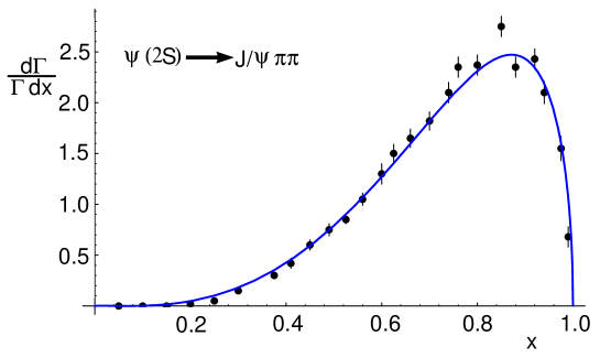
FIG. 1.: The normalized differential decay spectrum for $\psi(2S)\rightarrow J/\psi\pi^{+}\pi^{-}$ as function of scaled variable $x$. The solid curve is the fit at tree-level.

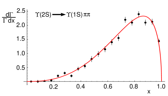
FIG. 2.: The normalized differential decay spectrum for $\Upsilon(2S)\rightarrow\Upsilon(1S)\pi^{+}\pi^{-}$ as function of scaled variable $x$. The solid curve is the fit at tree-level.

Note that the data we have shown in figs. 1 and 2 is taken directly from fig. 7 of reference[24]  and is not the original data set.

The partial-width for each decay modes is taken from the branching fractions and total width measurements of the $2S$ states given in particle data group evaluation [28]

$$\Gamma(\psi(2S)\rightarrow J/\psi\pi^{+}\pi^{-}) = 90\pm 10\ {\rm keV}$$ (37)

$$\Gamma(\Upsilon(2S)\rightarrow\Upsilon(1S)\pi^{+}\pi^{-}) = 8.1\pm 1.3\ {\rm keV}\ \ \ .$$ (38)

In what follows we will use only the central values of the above widths and neglect the uncertainties.

At leading order in the multipole expansion, and tree-level in the chiral lagrangian we can fit the parameters $C_{E}^{[(1S),(2S)]}$ and $C_{B}^{[(1S),(2S)]}$ (from now on we will drop the superscript, and simply use $C_{E}^{(\psi)}$, $C_{B}^{(\psi)}$ for the charmonium decays and $C_{E}^{(\Upsilon)}$, $C_{B}^{(\Upsilon)}$ for the $\Upsilon$ decays) to the spectra shown in fig.1 and fig. 2. The tree-level graphs in the chiral lagrangian that contribute to the decay are shown in fig. 3.

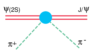
FIG. 3.: Tree-level diagrams contributing to $\psi(2S)\rightarrow J/\psi\pi^{+}\pi^{-}$. The light-shaded circle denotes insertions of $G^{2}$ and $T_{g}^{\mu\nu}$.

Using a value for the strong coupling of $\alpha_{s}(r_{c\overline{c}})=0.55$ for charmonium and $\alpha_{s}(r_{b\overline{b}})=0.33$ for bottomonium, we find ($V_{2}(\Lambda_{\chi})={1\over 2}$)

$$C_{E}^{(\psi)}-C_{B}^{(\psi)} = 7.0\pm 0.2\ {\rm GeV^{-3}}\ \ \ ,\ \ \ C_{E}^{(\psi)}+C_{B}^{(\psi)}=14\pm 1\ {\rm GeV^{-3}}$$ (39)

$$C_{E}^{(\Upsilon)}-C_{B}^{(\Upsilon)} = 1.3\pm 0.1\ {\rm GeV^{-3}}\ \ \ ,\ \ \ C_{E}^{(\Upsilon)}+C_{B}^{(\Upsilon)}=3.9\pm 0.7\ {\rm GeV^{-3}}\ \ \ .$$ (40)

In fitting the data we have weighted each data point equally (with an error of $\pm 0.1$) and not used the experimental uncertainty indicated by fig.1 and fig.2. We find a much tighter constraint on the difference between $C_{B}$ and $C_{E}$ (the coefficient of the $G^{2}$ operator) than on the sum (the coefficient of the $T_{g}^{\mu\nu}$ operator). These extractions then lead to

$$C_{E}^{(\psi)} = 10.5\pm 0.6\ {\rm GeV^{-3}}\ \ \ ,\ \ \ C_{B}^{(\psi)}=3.5\pm 0.5\ {\rm GeV^{-3}}$$ (41)

$$C_{E}^{(\Upsilon)} = 2.6\pm 0.4\ {\rm GeV^{-3}}\ \ \ ,\ \ \ C_{B}^{(\Upsilon)}=1.3\pm 0.3\ {\rm GeV^{-3}}\ \ \ .$$ (42)

We note that in fitting the data there is a global sign ambiguity in the coefficients $C_{E,B}$. We have chosen $C_{E}>0$ for our analysis. The uncertainties are from the fit only and do not include the uncertainty associated with the widths.

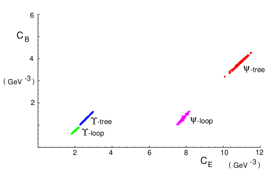
FIG. 4.: Tree-level and loop-level coefficients $C_{E}$ and $C_{B}$ for $\psi(2S)-J/\psi$ and $\Upsilon(2S)-\Upsilon(1S)$ systems. The $1-\sigma$ regions arise from a Monte-Carlo search in parameter space. We have used $V_{2}(\Lambda_{\chi})={1\over 2}$, $\alpha_{s}(r_{c\overline{c}})=0.55$ and $\alpha_{s}(r_{b\overline{b}})=0.33$. The loop-level fit is for $w_{4}=0$.

We see several interesting trends in these extractions. Firstly, the chromo-magnetic coefficient $C_{B}$ is significantly smaller than the chromo-electric coefficient $C_{E}$ for both systems. This is expected on grounds that the magnetic interaction should be suppressed by a power of the heavy quark three-velocity in the quarkonium. Secondly, both coefficients in the $\Upsilon$ system are substantially smaller than the corresponding quantity in the charmonium system. Again, this is to be expected on the grounds that the strong interactions will decouple in the limit of vanishing radius of the system. Our results at this order do not agree with results found in [19] where coefficients found in that work were approximately the same for both systems.

Fitting at one-loop is complicated by the fact that there are seven counterterms $w_{1}-w_{7}$. The counterterms $w_{1},w_{3},w_{5},w_{6}$ have only a small impact upon the decays under consideration as they are suppressed by powers of the $\pi$ mass compared to tree-level terms. The counterterm $w_{7}$ occurs in the trace of $T_{g}^{\mu\nu}$ at loop-level and as we have neglected the trace of $T_{g}^{\mu\nu}$ arising at loop-level (it is analytic in momenta and masses) we have set $w_{7}=0$. Naive dimensional analysis suggests that all the counterterms $w_{i}$ are of order unity, and hence the effects of setting each $w_{i}=0$ should be small. However, we find this not to be the case. It is clear from figs. 1 and 2 that the decays are well described at tree-level and additional momentum dependence arising at loop level will be small. As the amplitudes are dominated by the $G^{2}$ operator, we suspect and find that a non-zero value for the $w_{2}$ counterterm is required. With so many counterterms we can do little more than give examples.

As an explicit example, we set $w_{4}=0$ and have $w_{2}$ as the only counterterm to be fit to data. If the pion energy distributions became available then we would be able to fit both $w_{2}$ and $w_{4}$, but at present this is not possible. The counterterms $w_{1}$-$w_{7}$ are the same for all quarkonia systems, and we therefore simultaneously fit $C_{E}^{(\psi)},C_{B}^{(\psi)},C_{E}^{(\Upsilon)},C_{B}^{(\Upsilon)}$ and $w_{2}$ to the data sets for $\psi(2S)\rightarrow J/\psi\pi^{+}\pi^{-}$ and $\Upsilon(2S)\rightarrow\Upsilon(1S)\pi^{+}\pi^{-}$. The loop-level graphs in the chiral lagrangian that contribute to the decay are shown in fig. 5.

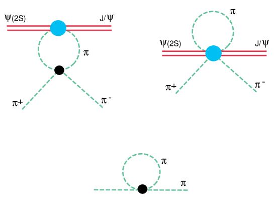
FIG. 5.: One-loop diagrams contributing to $\psi(2S)\rightarrow J/\psi\pi^{+}\pi^{-}$. The light-shaded circle denotes insertions of $G^{2}$ and $T_{g}^{\mu\nu}$. The dark circle denotes a strong interaction in the chiral lagrangian.

We find that

$$C_{E}^{(\psi)} = 7.8\pm 0.4\ {\rm GeV}^{-3}\ \ \ ,\ \ \ C_{B}^{(\psi)}=1.3\pm 0.3\ {\rm GeV}^{-3}$$ (43)

$$C_{E}^{(\Upsilon)} = 2.0\pm 0.2\ {\rm GeV}^{-3}\ \ \ ,\ \ \ C_{B}^{(\Upsilon)}=0.75\pm 0.14\ {\rm GeV}^{-3}$$ (44)

$$w_{2}(\Lambda_{\chi}) = -6.9\pm 0.4\ \ \ ,$$ (45)

where the errors on each quantity are correlated. It is comforting to see that the value of coefficients extracted at one-loop level are only slightly reduced from their tree-level extractions. One might fear that the relatively large momentum transfer involved in these processes $\sim 590\ {\rm MeV}$ may make the chiral expansion invalid, but it would appear that this is in fact not the case. However, there is a hint of a problem by the large value of $w_{2}$. The value of $w_{2}$ is such that it almost cancels the ${\cal O}(p^{4})$ contribution from the loop. It is interesting to note that for this fit we find that $C_{B}$ is much smaller than $C_{E}$ in the $\psi$-system. We are able to fit both the $\psi$ and $\Upsilon$ spectra with single counterterm that is independent of the quarkonium system. This suggests that higher order terms in the multipole expansion are small.

Fitting both $w_{2}$ and $w_{4}$ leads to a slightly better fit but the uncertainties associated with the parameters are large. The central values for the $C_{E,B}$ are very different from the tree-level extractions and one might worry that the expansion is breaking down, but the large uncertanties preclude any firm conclusions.

We note that others have looked at the role of final state interactions in these decays[29], but not using the framework of chiral perturbation theory.

V Comparison with the Large-$N_{c}$ Limit of QCD

One is presently unable to match directly from QCD onto the lagrange density involving quarkonia and gluons. Previous estimates of the interaction between quarkonia and light hadrons have been based largely on estimates of the various $C_{E}$ and $C_{B}$ in the large-$N_{c}$ limit of QCD [4, 5]. In the large-$N_{c}$ limit the repulsion in the colour octet channel vanishes as $1/N_{c}$ while the attraction in the singlet channel remains. Consequently, the colour octet intermediate state in the dominant diagrams in matching onto $C_{E}$ and $C_{B}$ can be described by plane waves. Further, the external color singlet states are coulombic. Matrix elements of a double insertion of the chromo-electric dipole operator are simply computed in terms of the overlap between coulomb bound-state wavefunctions and plane waves with a plane wave propogator. For zero-momentum transfer amplitudes this gives a sensible estimate for the actual matrix element, as there is a mass-gap between the intermediate state and the bound-state. However, for decay processes such as $\psi(2S)\rightarrow J/\psi\pi\pi$, the estimate is assured to be unreliable as the energy release is comparable to the gap between the bound state and the intermediate state(s).

At leading order there is no contribution to $C_{B}$ while there is a calculable contribution to $C_{E}$. For dipole-dipole interactions between the same initial and final states it is straightforward to show that [4, 5]

$$C_{E}^{[(nS),(nS)]} = {1\over 2}a_{0}^{3}d_{n}$$ (46)

$$d_{n} = {16\pi\over N_{c}^{2}}\ {1\over 3}\int{d^{3}k\over(2\pi)^{3}}{1\over k^{2}a_{0}^{2}+\epsilon/\epsilon_{0}}\left[{{\bf r^{i}}\over a_{0}}\Phi_{n}\right]^{*}(k)\left[{{\bf r^{i}}\over a_{0}}\Phi_{n}\right](k)\ \ \ ,$$ (47)

(${\bf i}$ is summed over) where $a_{0}$ is the bohr radius of the quarkonium ground state $a_{0}^{\psi}\sim(0.7\ {\rm GeV})^{-1}$, $a_{0}^{\Upsilon}\sim(1.5\ {\rm GeV})^{-1}$ [30]. The $\phi_{n}$ are coulomb wavefunctions for the n-th S-state, $\epsilon$ is the binding energy of the $n-th$ state and $\epsilon_{0}$ is the binding energy of the ground state. This calculation leads to

$$C_{E}^{[(1S),(1S)]} = a_{0}^{3}{14\pi\over 27}\ \ \ ,\ \ \ C_{B}^{[(1S),(1S)]}=0$$ (48)

$$C_{E}^{[(2S),(2S)]} = a_{0}^{3}{1004\pi\over 27}\ \ \ ,\ \ \ C_{B}^{[(2S),(2S)]}=0\ \ \ ,$$ (49)

which gives

$$C_{E}^{[(1S),(1S)]\psi} \sim 4.7\ ({\rm GeV})^{-3}\ \ \ ,\ \ \ C_{E}^{[(2S),(2S)]\psi}\sim 341\ ({\rm GeV})^{-3}$$ (50)

$$C_{E}^{[(1S),(1S)]\Upsilon} \sim 0.48\ ({\rm GeV})^{-3}\ \ \ ,\ \ \ C_{E}^{[(2S),(2S)]\Upsilon}\sim 35\ ({\rm GeV})^{-3}\ \ .$$ (51)

There is a problem in estimating the $C_{E,B}^{[(2S),(1S)]}$ from this construction from the fact that the energy release in the transition is the same magnitude as the off-shellness of the intermediate states in the free colour-octet propogator. In this limit a short-distance expansion makes little sense[20] and the operator-product expansion we have employed is inappropriate. However, it is more than likely that the colour-octet intermediate state has a mass splitting to the colour-singlet states, although the splitting does not become large in any limit of QCD. The splitting would allow one to perform the OPE as we have done and for the operators ${\cal O}_{E,B}$ to be the leading terms in a systematic expansion. As such, we cannot directly use the construction of the large-$N_{c}$ limit of QCD to make a reliable estimate of the $C_{E,B}^{[(2S),(1S)]}$. We can compare numerically the values of $C_{E,B}^{[(2S),(1S)]}$ we have obtained in previous sections and look to see if at least they are consistent. If we naively assume

$$C_{E,B}^{[(2S),(1S)]} \sim \sqrt{C_{E,B}^{[(1S),(1S)]}C_{E,B}^{[(2S),(2S)]}}\ \ \ ,$$ (52)

to provide an extremely rough estimate of what we might expect for the off-diagonal element, then we find that $C_{E}^{[(2S),(1S)]\psi}\sim 40({\rm GeV})^{-3}$ and $C_{E}^{[(2S),(1S)]\Upsilon}\sim 4({\rm GeV})^{-3}$ in the large-$N_{c}$ limit. These estimates are within factors of $\sim 4$ and $\sim 2$ of our extraction. From this we very cautiously hope that the large-$N_{c}$ estimates of the coefficients $C_{E,B}^{[(nS),(nS)]}$ are reasonably close to their true values and that the estimates for the binding energy of quarkonia in nuclear matter[10] are not unreasonable.

VI Applications

A Inelastic $\pi J/\psi\rightarrow\pi\psi(2S)$ and $\pi\Upsilon(1S)\rightarrow\pi\Upsilon(2S)$ Scattering

With the possibility of “$J/\psi$-suppression” being a tool for detecting the formation of a quark-gluon plasma in ultra-relativistic heavy ion collisions it is important to understand inelastic $J/\psi$ scattering in a gas of hadrons. Naively, one expects $\pi$’s to comprise a non-negligible fraction of the number density in a thermal hadronic gas, and as such, $\pi J/\psi$ inelastic scattering needs to be understood as a background to other mechanisms that remove the $J/\psi$’s produced in any given collision.

For $\pi J/\psi\rightarrow\pi\psi(2S)$ and $\pi\Upsilon(1S)\rightarrow\pi\Upsilon(2S)$ near threshold ($E_{\pi}^{\rm lab}\sim 810\ {\rm MeV}$) we can use directly the expression for ${\cal A}_{G}$ and ${\cal A}_{T}^{\mu\nu}$ discussed previously. It is likely that there will be significant corrections to the amplitudes for $\pi J/\psi\rightarrow\pi\psi(2S)$ and $\pi\Upsilon(1S)\rightarrow\pi\Upsilon(2S)$ determined from the crossed channels $\Upsilon(2S)\rightarrow\Upsilon(1S)\pi^{+}\pi^{-}$ and $\psi(2S)\rightarrow J/\psi\pi^{+}\pi^{-}$ simply due to the large energy transfer involved and a break-down of the chiral expansion in this kinematic regime. We expect that the calculation will fail close to threshold and the difference between the cross-section as computed at tree-level and at one-loop level will give some feeling for the range of validity of the chiral expansion.

FIG. 6.: The total cross-section in millibarns for $\pi J/\psi\rightarrow\pi\psi(2S)$ as a function of the $\pi$ lab energy in GeV. The curves are evaluated at the value of parameters corresponding to the best fit to $\psi(2S)\rightarrow J/\psi\pi^{+}\pi^{-}$ at tree-level and loop-level (with $w_{2}=-6.9$ and the remaining $w_{i}=0$).

The curves in fig. 6 indicate that the loop-level and tree-level estimates are not so different even near where the expansion must fail. This should be taken with extreme caution. However, we see that the cross section is of the order of $10^{-2}$ mb in the region where the computation is most reliable.

B Radiative Decays $\psi(2S)\rightarrow J/\psi\pi^{+}\pi^{-}\gamma$ and $\Upsilon(2S)\rightarrow\Upsilon(1S)\pi^{+}\pi^{-}\gamma$

The radiative decays $\psi(2S)\rightarrow J/\psi\pi^{+}\pi^{-}\gamma$ and $\Upsilon(2S)\rightarrow\Upsilon(1S)\pi^{+}\pi^{-}\gamma$ are dominated by electromagnetic interactions of the $\pi$’s that are calculable with the chiral lagrangian outlined in the previous sections, after gauging with respect to the electromagnetic interaction. Operators involving the electromagnetic field-strength tensor $F^{\mu\nu}$ arising in the matching between QCD and the effective theory of quarkonium will be suppressed by two powers of the quarkonium radius. There will be higher dimension operators in the chiral lagrangian arising from matching the theory of quarkonia and gluons onto the chiral lagrangian and quarkonia. Such operators are suppressed by additional powers of the chiral symmetry breaking scale. The leading contributions to $\psi(2S)\rightarrow J/\psi\pi^{+}\pi^{-}\gamma$ and $\Upsilon(2S)\rightarrow\Upsilon(1S)\pi^{+}\pi^{-}\gamma$ occur at tree-level and hence we do not need to discuss the role of local counterterms at leading order. We note that the decays $\psi(2S)\rightarrow J/\psi\pi^{0}\pi^{0}\gamma$ and $\Upsilon(2S)\rightarrow\Upsilon(1S)\pi^{0}\pi^{0}\gamma$ are forbidden by charge conjugation.

One might naively expect a significant contribution to the $\pi\pi\gamma$ decays from pole graphs with $\chi_{c0}(1P)$, $\chi_{c1}(1P)$ and $\chi_{c2}(1P)$ as intermediate states. However, G-parity forbids the $\chi_{cn}(1P)\rightarrow J/\psi\pi\pi$ transitions and therefore, such contributions are not present.

It is straightforward to determine the tree-level matrix element for the radiative decays. There are contributions from both the $G^{2}$ operator and the $T_{g}^{\mu\nu}$ operator as shown in fig.7.

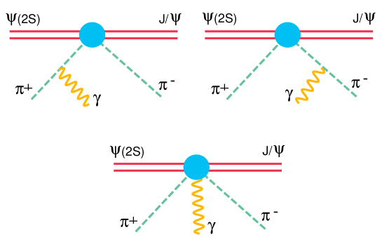
FIG. 7.: The tree-level diagrams contributing to $\psi(2S)\rightarrow J/\psi\pi^{+}\pi^{-}\gamma$. The light shaded circle denotes insertions of the $G^{2}$ and $T_{g}^{\mu\nu}$ operators.

The $G^{2}$ operator yields an amplitude of

$$i{\cal R}_{G} = ie\left(3m_{\pi}^{2}+2p_{+}\cdot p_{-}+2k\cdot(p_{+}+p_{-})\right)\left({p_{+}\cdot\varepsilon\over k\cdot p_{+}}-{p_{-}\cdot\varepsilon\over k\cdot p_{-}}\right)\ \ \ \ ,$$ (53)

where $k$ is the photon momentum, $p_{+,-}$ is the $\pi^{+,-}$ momentum resp., and $\varepsilon$ is the photon polarization tensor. The contribution from $T_{g}^{\mu\nu}$ is found to be

$$i{\cal R}_{T} = -2ieV_{2}(\mu)\left[v\cdot p_{-}\left({v\cdot kp_{+}\cdot\varepsilon\over p_{+}\cdot k}-v\cdot\varepsilon\right)-v\cdot p_{+}\left({v\cdot kp_{-}\cdot\varepsilon\over p_{-}\cdot k}-v\cdot\varepsilon\right)\right.$$ (55)

$$\left.+\left(v\cdot p_{+}v\cdot p_{-}-{1\over 4}p_{+}\cdot p_{-}-{1\over 4}k\cdot(p_{+}+p_{-})\right)\left({p_{+}\cdot\varepsilon\over k\cdot p_{+}}-{p_{-}\cdot\varepsilon\over k\cdot p_{-}}\right)\right]\ \ \ \ .$$

The full amplitude at this order is given by

$$i{\cal A}_{\gamma} = (C_{E}+C_{B})\left[i{\cal R}_{T}\right]\ +\ (C_{B}-C_{E}){g\over 2\beta(g)}\left[i{\cal R}_{G}\right]\ \ \ \ .$$ (56)

The distribution $d\Gamma/dY$ resulting from $i{\cal A}_{\gamma}$ as a function of the normalized photon energy $Y=E_{\gamma}/E_{\gamma}^{\rm max.}$ ($E_{\gamma}^{\rm max.}=309\ {\rm MeV}$) is shown for different values of the coefficients $C_{E}$ and $C_{B}$ in fig.8. In fig.9 we have shown the same differential spectrum weighted with the square of the normalized photon energy to highlight the higher energy part of the distribution. Experimentally verifying the differential distribution will be a good test of the chiral and multipole expansions.

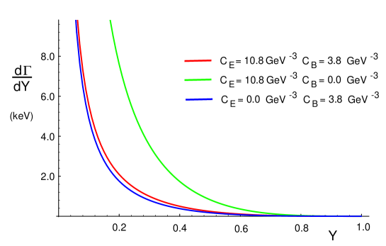
FIG. 8.: Differential decay spectrum as a function of normalized photon energy in $\psi(2S)\rightarrow J/\psi\pi^{+}\pi^{-}\gamma$. Shown are the distributions obtained for different values of $C_{E}$ and $C_{B}$.

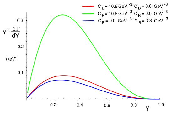
FIG. 9.: Differential decay spectrum as a function of normalized photon energy in $\psi(2S)\rightarrow J/\psi\pi^{+}\pi^{-}\gamma$ weighted with $Y^{2}$. Shown are the distributions for different values of $C_{E}$ and $C_{B}$.

The integrated branching fraction is infrared divergent as we have not included one-loop vertex and wavefunction graphs. However, it is useful to have the branching fraction for events with a $E_{\gamma}$ greater than some lower energy $E_{\gamma}^{\rm min}$.

$Y_{\rm min}$	Branching Fraction
0.2	$1.0\times 10^{-3}$
$0.4$	$2.2\times 10^{-4}$
$0.6$	$3.5\times 10^{-5}$
$0.8$	$1.8\times 10^{-6}$

TABLE I.: Branching fractions for $\psi(2S)\rightarrow J/\psi\pi^{+}\pi^{-}\gamma$ for different cuts on the normalized photon energy, $Y_{\rm min}$, for $\alpha_{s}(r_{c\overline{c}})=0.55$, $C_{E}=10.8\ {\rm GeV}^{-3}$ and $C_{B}=3.8\ {\rm GeV}^{-3}$.

In table 1 we have given the branching fraction for different values of $Y_{\rm min}$ for the tree-level extracted values of $C_{E}=10.8\ {\rm GeV}^{-3}$ and $C_{B}=3.8\ {\rm GeV}^{-3}$.

C Electromagnetic Polarizability of Quarkonia

While it is more than likely that the electromagnetic polarizability of quarkonia will never be measured, there is an interesting theoretical point to be discussed. The leading contribution to both the electric and magnetic polarizabilities, defined by an effective lagrange density,

$${\cal L}^{\rm eff.} = \sum_{v}\ \left(P^{\dagger}_{v}(f)P_{v}(i)-V^{\dagger}_{\mu v}(f)V^{\mu}_{v}(i)\right)\left[-2\pi(\alpha+\beta)v_{\sigma}v_{\rho}F^{\sigma\delta}F^{\rho}_{\delta}\ +\ \pi\beta F^{\sigma\delta}F_{\sigma\delta}\right]\ \ \ ,$$ (57)

comes from tree-level pole graphs, where two photons are coupled to the quarkonium via colour-singlet intermediate states. The constants $\alpha$ and $\beta$ are the electric and magnetic susceptibilities. Such contributions are finite in the chiral limit and are naively estimated to be

$$\alpha\sim\beta \sim {\alpha_{e}\over\pi\alpha_{s}(r_{Q\overline{Q}})}r_{Q\overline{Q}}^{3}\ \ \ ,$$ (58)

in the same way that $C_{E,B}$ are estimated in the large-$N_{c}$ limit. However, there is a contribution to $\alpha$ and $\beta$ from $C_{E}$ and $C_{B}$ via $\pi$ loops coupled to two photons, as shown in fig. 10.

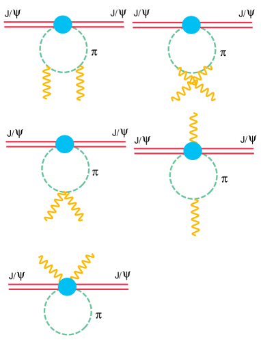
FIG. 10.: Diagrams contributing to the electromagnetic polarizabilities of the $J/\psi$. The shaded circle denotes insertions of $G^{2}$ and $T_{g}^{\mu\nu}$.

This is numerically subleading to the contribution from the pole graphs, except in the extreme chiral limit. In this limit the loop graphs are logarithmically infrared divergent,

$$\alpha^{\rm loop} = \beta^{\rm loop}=-{1\over 12\pi}V_{2}(\mu)(C_{E}+C_{B}){\alpha_{e}\over 4\pi}\log\left({m_{\pi}^{2}\over\Lambda_{\chi}^{2}}\right)\ \ \ ,$$ (59)

and only $T_{g}^{\mu\nu}$ contributes. Using the large-$N_{c}$ estimates of $C_{E}=4.7\ {\rm GeV}^{-3}$ and $C_{B}=0\ {\rm GeV}^{-3}$ along with the actual value of the $\pi$ mass and $V_{2}(\mu)={1\over 2}$, one finds a loop contribution of $\alpha^{\rm loop}=\beta^{\rm loop}\sim 10^{-6}\ {\rm fm^{3}}$.

D Decays from the $\Upsilon(3S)$

Until this point we have been considering decays from the $2S$ states in the $\psi$ and $\Upsilon$ systems. However, there is data available for the transitions $\Upsilon(3S)\rightarrow\Upsilon(1S)\pi\pi$ as shown in fig. 11, and $\Upsilon(3S)\rightarrow\Upsilon(2S)\pi\pi$ [26].

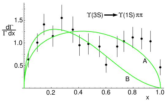
FIG. 11.: Spectrum for $\Upsilon(3S)\rightarrow\Upsilon(1S)\pi^{+}\pi^{-}$ verses $x$. The solid curve B shows the best tree-level fit for the data with $m_{\pi\pi}<0.65{\rm GeV}$, while curve A is the best fit over all $x$.

(Note that we have taken the data from fig. 11 of [26] and it is not the original data set.) The spectrum for $\Upsilon(3S)\rightarrow\Upsilon(2S)\pi\pi$ is similar to that of the decays from the $2S$ states and we will not discuss it further. There has been significant discussion of $\Upsilon(3S)\rightarrow\Upsilon(1S)\pi\pi$ as the differential spectrum does not have the same shape as that of transitions from the $2S$ states [29, 31, 32]. It has been suggested that a resonance in the $\Upsilon(1S)\pi$ channel [29, 31] is responsible for the observed distribution. Another suggestion was that the multipole expansion is subdominant to hadronic effects involving B-mesons[32]. It is important to note that the invariant mass of the $\pi\pi$ system can extend up to $0.9\ {\rm GeV}$. The soft pion analysis is expected to fail for the higher mass pairs. As such, one might expect to see modifications to the differential spectrum before the end-point. Further, it was assumed that $C_{B}$ vanished in the previous analyses, allowing only for a spectrum peaked near the high end of the spectrum. It is clear from fig. 11 that the best tree-level fit to the entire range of $x$ is poor, with the apparent minimum at $x\sim 0.6$ not reproduced. If we restrict ourselves to the low end of the spectrum where the chiral lagrangian is expected to be applicable, then that portion of the spectrum can be described with the multipole expansion. $T_{g}^{\mu\nu}$ dominates the decay amplitude with $C_{E}\sim C_{B}\sim 0.3$ yielding the best fit for $m_{\pi\pi}<0.65{\rm GeV}$. Clearly, only a portion of the spectrum can be described at leading order in the multipole and chiral expansions. Whether the deviations from the leading result arises from higher order terms in the chiral or multipole expansions or from a given resonance cannot be determined. However, in order to reproduce the low-mass region of the spectrum, a large value for the chromo-magnetic coupling $C_{B}$ is required, in contrast to transitions from the $2S$ states.

VII Discussion

We have explored the strong interactions and radiative decays of quarkonia in order to better understand the multipole and chiral expansions that might be appropriate for such processes. The unproven convergence of the multipole expansion is assumed throughout this work and we suggest that numerical factors could lead to convergence despite there being no rigorous limit of QCD in which this is true. Current discussions of how quarkonia interact with the light hadrons away from the chiral limit have been addressed and the strong decays $\psi(2S)\rightarrow J/\psi\pi^{+}\pi^{-}$, $\Upsilon(2S)\rightarrow\Upsilon(1S)\pi^{+}\pi^{-}$ were focused on at tree-level and loop-level in the chiral expansion. The leading couplings in the multipole expansion are found to be significantly smaller in the $\Upsilon$ system than in the $\psi$ system, consistent with naive scaling arguments. Further, counterterms appearing at loop level in the chiral expansion are found to be approximately the same for the $\psi$ and $\Upsilon$ systems, suggesting that the multipole expansion is converging. In addition, we discussed the large-$N_{C}$ limit in which estimates of the coefficients $C_{E,B}$ for various quarkonium states have been made. While there is nothing concrete that can be concluded, it would appear that the large-$N_{C}$ limit is not in serious conflict with data. Crossing symmetry has been used to estimate the size of the inelastic $\pi J/\psi\rightarrow\pi\psi(2S)$ scattering cross section that might be relevant for understanding $\psi$ suppression in ultra-relativistic heavy ion collisions. In the region where the theory is expected to be most reliable we find a small cross section, $\sim 10^{-2}\ {\rm mb}$. Power counting in the quarkonium radius indicates that the radiative decays $\psi(2S)\rightarrow J/\psi\pi^{+}\pi^{-}\gamma$, $\Upsilon(2S)\rightarrow\Upsilon(1S)\pi^{+}\pi^{-}\gamma$ are dominated by tree graphs computable in chiral perturbation theory. The photon energy spectrum is presented and branching fractions $\sim 10^{-4}$ are found. These branching fraction depends sensitively upon the values of $C_{E,B}$ used and thus provides a consistency test of the calculational framework. Finally, we made brief remarks on transitions from the $\Upsilon(3S)$ and on the electromagnetic polarizability of the $\psi$.

Acknowledgements

We would like to thank Jerry Miller for discussions that lead to this work. We also thank M. Luke for his critical reading of the manuscript. This work is supported by the Department of Energy.

REFERENCES

- [1] K. Gottfried, Phys. Rev. Lett. 40 (1978) 538.
- [2] M. Voloshin and V. Zakharov, Phys. Rev. Lett. 45 (1980) 688.
- [3] M. Voloshin, Nucl. Phys. B154 (1979) 365.
- [4] M. Peskin, Nucl. Phys. B156 (1979) 365.
- [5] G. Bhanot and M. Peskin, Nucl. Phys. B156 (1979) 391.
- [6] V.A. Novikov and M.A. Shifman, Z. Phys. C8 (1981) 43.
- [7] Y.-P. Kuang and T.-M. Yan, Phys. Rev. D22 (1980) 1652.
- [8] T.-M. Yan, Phys. Rev. D24 (1981) 2874.
- [9] S.J. Brodsky, I. Schmidt and G.F. de Teramond, Phys. Rev. Lett. 64 (1990) 1011.
- [10] M. Luke, A.V. Manohar and M.J. Savage, Phys.Lett. B288 (1992) 355-359.
- [11] A.B. Kaidalov and P.E. Volkovitsky, Phys. Rev. Lett. 69 (1992) 3155.
- [12] S.J. Brodsky and G.A. Miller, hep-ph/9707382 (1997), to appear in PLB.
- [13] E. Crosbie et al, Phys. Rev. D23 (1981) 600.
- [14] S. Brodsky and G.F. de Teramond, Phys. Rev. Lett. 60 (1988) 1924.
- [15] T. Matsui and H. Satz, Phys. Lett. B178 (1986) 416.
- [16] S. Gavin and R. Vogt, Phys.Rev.Lett. 78 (1997) 1006.
- [17] L.S. Brown and R.N. Cahn, Phys. Rev. Lett. 35 (1975) 1.
- [18] B. Grinstein and I. Rothstein, Phys. Lett. B385 (1996) 265.
- [19] T. Mannel and R. Urech, Z. Phys C 73 (1997) 541.
- [20] M. Luty and R. Sundrum, Phys.Lett. B312 (1993) 205-210.
- [21] R.S. Chivukula et al, Annals of Phys. 192 (1989) 93.
- [22] D. Kharzeev, CERN-TH-95-342, nucl-th/9601029 (1996).
- [23] M. Gluck, E. Reya and A. Vogt, Z. Phys. C53 (1992) 651.
- [24] H. Albrecht et al (ARGUS Collaboration), Z. Phys. 35 (1987) 283.
- [25] T.M. Himel: (thesis), SLAC-223 (1979), as presented in [24].
- [26] F. Butler et al, Phys.Rev. D49 (1994) 40.
- [27] P. Moxhay, Phys. Rev. D39 (1989) 3497.
- [28] L. Montanet et al (Particle Data Group), Phys.Rev. D50 (1994) 1173.
- [29] G. Belanger, T. DeGrand and P. Moxhay, Phys. Rev. 39 (1989) 257.
- [30] C. Quigg and J. L. Rosner, Phys. Rev. D23 (1981) 2625.
- [31] M.B. Voloshin, JETP Lett. 37 (1983) 69.
- [32] H.J. Lipkin and S.F. Tuan, Phys. Lett. B206 (1988) 349.