CERN-TH/97-281

Extended version

hep-ph/9710331

Towards Extractions of the CKM Angle $\gamma$ from
$B_{u,d}\to\pi K$ and Untagged $B_{s}\to K\overline{K}$ Decays

Robert Fleischer

Theory Division, CERN, CH-1211 Geneva 23, Switzerland

The decays $B_{d}\to\pi^{\mp}K^{\pm}$ and $B^{\pm}\to\pi^{\pm}K$ provide interesting constraints on the angle $\gamma$ of the unitarity triangle of the CKM matrix. It is shown that bounds on $\gamma$ can also be obtained from the time evolution of untagged $B_{s}\to K^{+}K^{-}$ and $B_{s}\to K^{0}\overline{K^{0}}$ decays, provided the $B_{s}$ system exhibits a sizeable width difference $\Delta\Gamma_{s}$. A detailed discussion of rescattering processes and electroweak penguin effects, which limit the theoretical accuracy of these constraints, and of methods to control them through experimental data is given. Moreover, strategies are pointed out to go beyond these bounds by relating the $B_{u,d}\to\pi K$ and untagged $B_{s}\to K\overline{K}$ decays through the $SU(3)$ flavour symmetry of strong interactions. If a tagged, time-dependent measurement of the $B_{s}\to K^{+}K^{-}$ and $B_{s}\to K^{0}\overline{K^{0}}$ modes should become possible, $\gamma$ could be determined from the corresponding observables in a way that makes use of only the $SU(2)$ isospin symmetry and takes into account rescattering effects “automatically”. The impact of new-physics contributions to $B^{0}_{s}$–$\overline{B^{0}_{s}}$ mixing is also analysed, and interesting features arising in such a scenario of physics beyond the Standard Model are pointed out.

CERN-TH/97-281
Extended version
April 1998

1 Introduction

The determination of the angle $\gamma$ of the usual non-squashed unitarity triangle [1] of the Cabibbo–Kobayashi–Maskawa matrix (CKM matrix) [2] is considered as being very challenging from an experimental point of view [3]. In order to accomplish this ambitious task, the decays $B^{0}_{d}\to\pi^{-}K^{+}$, $B^{+}\to\pi^{+}K^{0}$ and their charge conjugates are very promising and have received considerable interest in the recent literature [4]–[8]. These modes, which have recently been observed by the CLEO collaboration [9], should allow us to obtain direct information on the CKM angle $\gamma$ at future $B$-factories (BaBar, BELLE, CLEO III) (for interesting feasibility studies, see [6, 7, 10]). At present, there are only experimental results available for the following combined branching ratios [9]:

$$\mbox{BR}(B_{d}\to\pi^{\mp}K^{\pm}) \equiv \frac{1}{2}\left[\mbox{BR}(B^{0}_{d}\to\pi^{-}K^{+})+\mbox{BR}(\overline{B^{0}_{d}}\to\pi^{+}K^{-})\right]$$ (1)

$$= \left(1.5^{+0.5}_{-0.4}\pm 0.1\pm 0.1\right)\times 10^{-5}$$

$$\mbox{BR}(B^{\pm}\to\pi^{\pm}K) \equiv \frac{1}{2}\left[\mbox{BR}(B^{+}\to\pi^{+}K^{0})+\mbox{BR}(B^{-}\to\pi^{-}\overline{K^{0}})\right]$$ (2)

$$= \left(2.3^{+1.1}_{-1.0}\pm 0.3\pm 0.2\right)\times 10^{-5}.$$

In order to determine the CKM angle $\gamma$, the separate branching ratios for $B^{0}_{d}\to\pi^{-}K^{+}$, $B^{+}\to\pi^{+}K^{0}$ and their charge conjugates are needed, i.e. the combined branching ratios (1) and (2) are not sufficient, and an additional input is required to fix the magnitude of a certain decay amplitude $T$, which is usually referred to as a “tree” amplitude and will be discussed in more detail below [4, 6, 7]. Using arguments based on “factorization” [11], one expects that a future theoretical uncertainty of $|T|$ as small as ${\cal O}(10\%)$ may be achievable. Since detailed studies show that the properly defined amplitude $T$ is actually not just a colour-allowed “tree” amplitude, where “factorization” may work reasonably well [12], but that it receives also contributions from penguin and annihilation topologies due to certain rescattering effects [8, 13], these expectations appear too optimistic. In any case, some model dependence enters in the extracted value of $\gamma$.

As was pointed out in [5], it is in principle possible to obtain constraints on the CKM angle $\gamma$ that do not suffer from a model dependence related to $|T|$. To this end, the combined branching ratios (1) and (2) are sufficient. In general, such constraints, which take the form

$$0^{\circ}\leq\gamma\leq\gamma_{0}\quad\lor\quad 180^{\circ}-\gamma_{0}\leq\gamma\leq 180^{\circ},$$ (3)

depend also on $|T|$. However, if the ratio

$$R\equiv\frac{\mbox{BR}(B_{d}\to\pi^{\mp}K^{\pm})}{\mbox{BR}(B^{\pm}\to\pi^{\pm}K)}$$ (4)

of the combined $B_{u,d}\to\pi K$ branching ratios (1) and (2) is found to be smaller than 1 – its present experimental range is $0.65\pm 0.40$, so that this may indeed be the case – the bound $\gamma_{0}$ takes a maximal value, which is given by

$$\gamma_{0}^{\rm max}=\arccos(\sqrt{1-R})\,,$$ (5)

and depends only on $R$. The remarkable feature of these constraints is the fact that they exclude values of $\gamma$ around $90^{\circ}$, thereby providing complementary information to the present “indirect” range

$$41^{\circ}\mathrel{\hbox{\hbox to0.0pt{\hbox{\lower 4.0pt\hbox{$\sim$}}\hss}\hbox{$<$}}}\gamma\mathrel{\hbox{\hbox to0.0pt{\hbox{\lower 4.0pt\hbox{$\sim$}}\hss}\hbox{$<$}}}134^{\circ},$$ (6)

which arises from the usual fits of the unitarity triangle [14]. A detailed study of the implications of these bounds on $\gamma$ for the determination of the unitarity triangle can be found in [15]. Their theoretical accuracy is limited by certain rescattering processes and electroweak penguin effects, which led to considerable interest in the recent literature [16]–[20] (for earlier references, see [21]). A comprehensive analysis of these effects and strategies to control them through additional experimental data has recently been performed in [8].

In this paper, we focus on the modes $B_{s}\to K^{+}K^{-}$ and $B_{s}\to K^{0}\overline{K^{0}}$, which are the $B_{s}$ counterparts of the $B_{u,d}\to\pi K$ decays discussed above, where the up and down “spectator” quarks are replaced by a strange quark. Because of the expected large $B^{0}_{s}$–$\overline{B^{0}_{s}}$ mixing parameter $x_{s}\equiv\Delta M_{s}/\Gamma_{s}={\cal O}(20)$, experimental studies of CP violation in $B_{s}$ decays are regarded as being very difficult. In particular, an excellent vertex resolution system is required to keep track of the rapid oscillatory $\Delta M_{s}t$-terms arising in tagged $B_{s}$ decays. These terms cancel, however, in untagged $B_{s}$ decay rates, where one does not distinguish between initially present $B^{0}_{s}$ and $\overline{B^{0}_{s}}$ mesons. In that case, the expected sizeable width difference $\Delta\Gamma_{s}\equiv\Gamma_{H}^{(s)}-\Gamma_{L}^{(s)}$ between the mass eigenstates $B_{s}^{H}$ (“heavy”) and $B_{s}^{L}$ (“light”) of the $B_{s}$ system, which may be as large as ${\cal O}(20\%)$ of the average $B_{s}$ decay width $\Gamma_{s}$ [22], provides an alternative route to explore CP violation [23]. Several strategies have recently been proposed to extract CKM phases from such untagged $B_{s}$ decays [23]–[25] (for a review, see [26]).

In Ref. [24], it was pointed out that untagged data samples of the modes $B_{s}\to K^{+}K^{-}$ and $B_{s}\to K^{0}\overline{K^{0}}$ allow a determination of the CKM angle $\gamma$. As in the case of the $B_{u,d}\to\pi K$ transitions, to this end the magnitude of a certain “tree” amplitude $T_{s}$ has to be fixed, leading again to some model dependence of the extracted value of $\gamma$. The observables of the untagged $B_{s}\to K^{+}K^{-}$ and $B_{s}\to K^{0}\overline{K^{0}}$ modes provide, however, also constraints on $\gamma$, which do not depend on such an input. Their theoretical accuracy is also limited by certain rescattering and electroweak penguin effects, which will be investigated by following closely the formalism developed in [8].

The outline of this paper is as follows: in Section 2, we introduce a parametrization of the $B_{u,d}\to\pi K$ and $B_{s}\to K\overline{K}$ decay amplitudes in terms of “physical” quantities, and define the relevant observables. In Section 3, we discuss strategies to constrain and determine the CKM angle $\gamma$ with the help of these decays. A detailed discussion of rescattering processes and electroweak penguin effects, which limit the theoretical accuracy of these strategies, is given in Section 4. In Section 5, we point out that the methods to extract $\gamma$ from $B_{u,d}\to\pi K$ and $B_{s}\to K\overline{K}$ decays, which require knowledge of $|T|$ and $|T_{s}|$, can be combined by using the $SU(3)$ flavour symmetry of strong interactions. Following these lines, such an input can be avoided, and $|T|$ and $|T_{s}|$ can rather be determined as a “by-product”. In Section 6, we write a few words on a tagged analysis of the $B_{s}\to K\overline{K}$ modes, which would allow an extraction of $\gamma$ by using only the $SU(2)$ isospin symmetry of strong interactions, taking into account rescattering effects “automatically”. The impact of CP-violating new-physics contributions to $B^{0}_{s}$–$\overline{B^{0}_{s}}$ mixing for the observables of the $B_{s}\to K\overline{K}$ decays is analysed in Section 7, and the conclusions are given in Section 8.

2 Decay Amplitudes and Observables

The subject of this section is to introduce a general parametrization of the $B_{u,d}\to\pi K$ and $B_{s}\to K\overline{K}$ decay amplitudes in terms of “physical” quantities, and to define the relevant observables to obtain information on the CKM angle $\gamma$.

2.1 Decay Amplitudes

The case of the $B_{u,d}\to\pi K$ decays was discussed in detail in [8]. Using the $SU(2)$ isospin symmetry of strong interactions to relate QCD penguin topologies with internal top and charm quark exchanges (for subtleties related to QCD penguin topologies with internal up quarks, see [8, 13]), the $B^{+}\to\pi^{+}K^{0}$ and $B^{0}_{d}\to\pi^{-}K^{+}$ decay amplitudes can be expressed as follows:

$$A(B^{+}\to\pi^{+}K^{0}) = P$$ (7)

$$A(B^{0}_{d}\to\pi^{-}K^{+}) = -\,[P+T+P_{\rm ew}]\,,$$ (8)

where the quantity

$$P=-\left(1-\frac{\lambda^{2}}{2}\right)\lambda^{2}A\left[1+\rho\,e^{i\theta}e^{i\gamma}\right]{\cal P}_{tc}$$ (9)

with

$$\rho\,e^{i\theta}=\frac{\lambda^{2}R_{b}}{1-\lambda^{2}/2}\left[1-\left(\frac{{\cal P}_{uc}+{\cal A}}{{\cal P}_{tc}}\right)\right]$$ (10)

and

$${\cal P}_{tc} \equiv |{\cal P}_{tc}|e^{i\delta_{tc}}=\left(P_{t}-P_{c}\right)+\left(P_{\rm ew}^{t}-P_{\rm ew}^{c}\right)$$ (11)

$${\cal P}_{uc} \equiv |{\cal P}_{uc}|e^{i\delta_{uc}}=\left(P_{u}-P_{c}\right)+\left(P_{\rm ew}^{u}-P_{\rm ew}^{c}\right)$$ (12)

is usually referred to as a $\bar{b}\to\bar{s}$ “penguin” amplitude. In these expressions, $P_{q}$ and $P_{\rm ew}^{q}$ denote the contributions of QCD and electroweak penguin topologies with internal $q$ quarks $(q\in\{u,c,t\})$ to $B^{+}\to\pi^{+}K^{0}$, respectively, $\delta_{uc}$, $\delta_{tc}$, and $\theta$ are CP-conserving strong phases, the amplitude ${\cal A}$ is due to annihilation processes, and

$$\lambda\equiv|V_{us}|=0.22\,,\quad A\equiv\frac{1}{\lambda^{2}}\left|V_{cb}\right|=0.81\pm 0.06\,,\quad R_{b}\equiv\frac{1}{\lambda}\left|\frac{V_{ub}}{V_{cb}}\right|=0.36\pm 0.08$$ (13)

are the relevant CKM factors, expressed in terms of the Wolfenstein parameters [27]. The amplitudes $T$ and $P_{\rm ew}$ – the latter is essentially due to electroweak penguins – can be parametrized as follows [8]:

$$T\equiv e^{i\delta_{T}}e^{i\gamma}|T|=\lambda^{4}A\,R_{b}\,e^{i\gamma}\left[\tilde{\cal T}-{\cal A}+\left(\tilde{P}_{u}-P_{u}\right)+\left(\tilde{P}_{\rm ew}^{u}-\tilde{P}_{\rm ew}^{t}\right)-\left(P_{\rm ew}^{u}-P_{\rm ew}^{t}\right)\right]$$ (14)

$$P_{\rm ew}\equiv-\,|P_{\rm ew}|\,e^{i\delta_{\rm ew}}=-\left(1-\frac{\lambda^{2}}{2}\right)\lambda^{2}A\left[\left(\tilde{P}_{\rm ew}^{t}-\tilde{P}_{\rm ew}^{c}\right)-\left(P_{\rm ew}^{t}-P_{\rm ew}^{c}\right)\right],$$ (15)

where the tildes have been introduced to distinguish the $B^{0}_{d}\to\pi^{-}K^{+}$ amplitudes from those contributing to $B^{+}\to\pi^{+}K^{0}$, and $\delta_{T}$ and $\delta_{\rm ew}$ are CP-conserving strong phases. In the literature, $T$ is usually referred to as a colour-allowed $\bar{b}\to\bar{u}u\bar{s}$ “tree” amplitude. This terminology is, however, misleading in this case, since $T$ receives actually not only “tree” contributions, which are described by $\tilde{\cal T}$, but also contributions from penguin and annihilation topologies, as can be seen in (14) [8, 13]. The expressions for the charge-conjugate decays $B^{-}\to\pi^{-}\overline{K^{0}}$ and $\overline{B^{0}_{d}}\to\pi^{+}K^{-}$ can be obtained straightforwardly from (7) and (8) by performing the substitution $\gamma\to-\,\gamma$ in (9) and (14).

The $B^{0}_{s}\to K^{0}\overline{K^{0}}$ and $B^{0}_{s}\to K^{+}K^{-}$ decay amplitudes take a completely analogous form to (7) and (8):

$$A(B^{0}_{s}\to K^{0}\overline{K^{0}}) = P_{s}$$ (16)

$$A(B^{0}_{s}\to K^{+}K^{-}) = -\,[P_{s}+T_{s}+P_{\rm ew}^{s}]\,.$$ (17)

In contrast to $B^{+}\to\pi^{+}K^{0}$, its $B_{s}$ counterpart $B^{0}_{s}\to K^{0}\overline{K^{0}}$ does not receive an annihilation amplitude corresponding to ${\cal A}$, while an “exchange” amplitude $\tilde{\cal E}_{s}$ contributes to $B^{0}_{s}\to K^{+}K^{-}$, which is not present in $B^{0}_{d}\to\pi^{-}K^{+}$. Moreover, in the case of the $B_{s}$ modes, we have not only to deal with “ordinary” penguin topologies, but also with “penguin annihilation” processes, which we denote, as the authors of [28], generically by the symbol $(PA)$. Consequently, we obtain the following expressions for $\rho_{s}\,e^{i\theta_{s}}$, $T_{s}$ and $P_{\rm ew}^{s}$:

$$\rho_{s}\,e^{i\theta_{s}}=\frac{\lambda^{2}R_{b}}{1-\lambda^{2}/2}\left[1-\left\{\frac{{\cal P}_{uc}^{s}+({\cal PA})_{uc}^{s}}{{\cal P}_{tc}^{s}+({\cal PA})_{tc}^{s}}\right\}\right]$$ (18)

$$T_{s}\equiv e^{i\delta_{T}^{s}}e^{i\gamma}|T_{s}|=\lambda^{4}A\,R_{b}\,e^{i\gamma}\biggl{[}\tilde{\cal T}_{s}+\tilde{\cal E}_{s}+\left\{\tilde{P}_{u}^{s}+(\widetilde{PA})_{u}^{s}-P_{u}^{s}-(PA)_{u}^{s}\right\}$$

$$+\left\{\tilde{P}_{\rm ew}^{u(s)}+(\widetilde{PA})_{\rm ew}^{u(s)}-\tilde{P}_{\rm ew}^{t(s)}-(\widetilde{PA})_{\rm ew}^{t(s)}\right\}\,-\,\left\{P_{\rm ew}^{u(s)}+(PA)_{\rm ew}^{u(s)}-P_{\rm ew}^{t(s)}-(PA)_{\rm ew}^{t(s)}\right\}\biggr{]}$$

$$P_{\rm ew}^{s}\equiv-\,|P_{\rm ew}^{s}|\,e^{i\delta_{\rm ew}^{s}}=-\left(1-\frac{\lambda^{2}}{2}\right)\lambda^{2}A$$

$$\times\left[\left\{\tilde{P}_{\rm ew}^{t(s)}+(\widetilde{PA})_{\rm ew}^{t(s)}-\tilde{P}_{\rm ew}^{c(s)}-(\widetilde{PA})_{\rm ew}^{c(s)}\right\}\,-\,\left\{P_{\rm ew}^{t(s)}+(PA)_{\rm ew}^{t(s)}-P_{\rm ew}^{c(s)}-(PA)_{\rm ew}^{c(s)}\right\}\right].$$

In order to distinguish the $B^{0}_{s}\to K^{0}\overline{K^{0}}$ decay amplitudes from those contributing to $B^{0}_{s}\to K^{+}K^{-}$, we have introduced, as in the $B_{u,d}\to\pi K$ case, tildes to label the latter.

The expected hierarchy of the various contributions to the $B_{u,d}\to\pi K$ and $B_{s}\to K\overline{K}$ modes and the impact of rescattering processes will be discussed in Section 4. For the following considerations, the amplitude relations given in (7), (8) and (16), (17) are of particular interest. As was pointed out in [8], the amplitudes $\rho\,e^{i\theta}$, $T$ and $P_{\rm ew}$ are properly defined “physical” quantities. A similar comment applies to their $B_{s}$ counterparts.

2.2 Observables

In order to obtain information on the CKM angle $\gamma$ from the decays $B^{+}\to\pi^{+}K^{0}$, $B^{0}_{d}\to\pi^{-}K^{+}$ and their charge conjugates, the following observables play a key role [8]:

$$R \equiv \frac{\mbox{BR}(B_{d}\to\pi^{\mp}K^{\pm})}{\mbox{BR}(B^{\pm}\to\pi^{\pm}K)}=1\,-\,2\,\frac{r}{w}\,\left[\,\cos\delta\cos\gamma+\rho\,\cos(\delta-\theta)\,\right]+r^{2}$$ (21)

$$+\,2\,\frac{\epsilon}{w}\,\left[\,\cos\Delta+\rho\,\cos(\Delta-\theta)\cos\gamma\,\right]\,-\,2\,r\,\epsilon\,\cos(\delta-\Delta)\cos\gamma+\epsilon^{2}$$

$$A_{0} \equiv \frac{\mbox{BR}(B^{0}_{d}\to\pi^{-}K^{+})-\mbox{BR}(\overline{B^{0}_{d}}\to\pi^{+}K^{-})}{\mbox{BR}(B^{+}\to\pi^{+}K^{0})+\mbox{BR}(B^{-}\to\pi^{-}\overline{K^{0}})}=A_{\rm CP}(B_{d}\to\pi^{\mp}K^{\pm})\,R$$ (22)

$$=A_{+}+2\,\frac{r}{w}\,\sin\delta\sin\gamma+2\,r\,\epsilon\sin(\delta-\Delta)\sin\gamma+2\,\epsilon\,\frac{\rho}{w}\,\sin(\Delta-\theta)\sin\gamma\,,$$

where

$$A_{+}\equiv\frac{\mbox{BR}(B^{+}\to\pi^{+}K^{0})-\mbox{BR}(B^{-}\to\pi^{-}\overline{K^{0}})}{\mbox{BR}(B^{+}\to\pi^{+}K^{0})+\mbox{BR}(B^{-}\to\pi^{-}\overline{K^{0}})}=-\,2\,\frac{\rho}{w^{2}}\,\sin\theta\sin\gamma$$ (23)

measures direct CP violation in the decay $B^{+}\to\pi^{+}K^{0}$, and

$$w\equiv\sqrt{1+2\,\rho\,\cos\theta\cos\gamma+\rho^{2}}\,.$$ (24)

In (21) and (22), we have introduced the CP-conserving strong phase differences

$$\delta\equiv\delta_{T}-\delta_{tc}\,,\quad\Delta\equiv\delta_{\rm ew}-\delta_{tc}\,,$$ (25)

and the quantities

$$r\equiv\frac{|T|}{\sqrt{\left\langle|P|^{2}\right\rangle}}\,,\quad\epsilon\equiv\frac{|P_{\rm ew}|}{\sqrt{\left\langle|P|^{2}\right\rangle}}\,,$$ (26)

where

$$\left\langle|P|^{2}\right\rangle\equiv\frac{1}{2}\left(|P|^{2}+|\overline{P}|^{2}\right).$$ (27)

Note that tiny phase-space effects have been neglected in (21) and (22) (for a detailed discussion, see [5]).

In the case of the modes $B_{s}\to K^{0}\overline{K^{0}}$ and $B_{s}\to K^{+}K^{-}$, we have to deal with $B_{s}$ decays into final states, which are eigenstates of the CP operator. Taking into account the interference effects arising from $B^{0}_{s}$–$\overline{B^{0}_{s}}$ mixing, the time evolution of the corresponding untagged decay rates, which are defined by

$$\Gamma[f(t)]\equiv\Gamma(B_{s}^{0}(t)\to f)\,+\,\Gamma(\overline{B^{0}_{s}}(t)\to f)\,,$$ (28)

where $\Gamma(B_{s}^{0}(t)\to f)$ and $\Gamma(\overline{B^{0}_{s}}(t)\to f)$ denote the transition rates corresponding to initially, i.e. at time $t=0$, present $B_{s}^{0}$ and $\overline{B^{0}_{s}}$ mesons, takes the following form [3]:

$$\Gamma[f(t)]\propto\left[\left(\frac{1+|\xi_{f}|^{2}}{2}\right)-\,\mbox{Re}\,(\xi_{f})\right]e^{-\Gamma_{L}^{(s)}t}+\left[\left(\frac{1+|\xi_{f}|^{2}}{2}\right)+\mbox{Re}\,(\xi_{f})\right]e^{-\Gamma_{H}^{(s)}t}.$$ (29)

The observable

$$\xi_{f}=-\,\eta_{\rm CP}^{f}\,e^{-i\phi_{\rm M}^{(s)}}\,\frac{A(\overline{B^{0}_{s}}\to f)}{A(B^{0}_{s}\to f)}$$ (30)

is proportional to the ratio of the unmixed decay amplitudes $A(\overline{B^{0}_{s}}\to f)$ and $A(B^{0}_{s}\to f)$, and $\eta_{\rm CP}^{f}$ denotes the CP eigenvalue of the final state $f$. The weak $B^{0}_{s}$–$\overline{B^{0}_{s}}$ mixing phase $\phi_{\rm M}^{(s)}=2\,\mbox{arg}(V_{ts}^{\ast}V_{tb})$ is negligibly small in the Standard Model.

If we use the parametrization of the $B_{s}\to K\overline{K}$ decay amplitudes discussed in the previous subsection, we obtain

$$\Gamma[K^{0}\overline{K^{0}}(t)] = R_{L}\,e^{-\Gamma_{L}^{(s)}t}\,+\,R_{H}\,e^{-\Gamma_{H}^{(s)}t}$$ (31)

$$\Gamma[K^{+}K^{-}(t)] = \Gamma[K^{0}\overline{K^{0}}(0)]\left[\,a\,e^{-\Gamma_{L}^{(s)}t}\,+\,b\,e^{-\Gamma_{H}^{(s)}t}\right].$$ (32)

Introducing the phase-space factor

$${\cal C}=\frac{1}{8\,\pi\,M_{B_{s}}}\sqrt{1-4\left(\frac{M_{K}}{M_{B_{s}}}\right)^{2}}\,,$$ (33)

the $B_{s}\to K^{0}\overline{K^{0}}$ observables are given by

$$R_{L} = \left(1+2\,\rho_{s}\,\cos\theta_{s}\cos\gamma+\rho_{s}^{2}\cos^{2}\gamma\right)\Gamma_{0}$$ (34)

$$R_{H} = \left(\rho_{s}^{2}\sin^{2}\gamma\right)\Gamma_{0}\,,$$ (35)

where

$$\Gamma_{0}={\cal C}\left[\left(1-\frac{\lambda^{2}}{2}\right)\lambda^{2}A\left|{\cal P}_{tc}^{s}+({\cal PA})_{tc}^{s}\right|\right]^{2}.$$ (36)

The untagged $B_{s}\to K^{0}\overline{K^{0}}$ decay rate allows us to fix $\left\langle|P_{s}|^{2}\right\rangle$, which is defined in analogy to (27), through

$${\cal C}\left\langle|P_{s}|^{2}\right\rangle=\Gamma[K^{0}\overline{K^{0}}(0)]=R_{L}+R_{H}\,.$$ (37)

Consequently, in order to parametrize the untagged $B_{s}\to K^{+}K^{-}$ rate, we may introduce quantities $r_{s}$ and $\epsilon_{s}$ as in (26), i.e.

$$r_{s}\equiv\frac{|T_{s}|}{\sqrt{\left\langle|P_{s}|^{2}\right\rangle}}\,,\quad\epsilon_{s}\equiv\frac{|P_{\rm ew}^{s}|}{\sqrt{\left\langle|P_{s}|^{2}\right\rangle}}\,,$$ (38)

and obtain

$$a=1-2\,\frac{r_{s}}{w_{s}}\,\left[\,\cos\delta_{s}\cos\gamma+\rho_{s}\,\cos(\delta_{s}-\theta_{s})\cos^{2}\gamma\,\right]+r_{s}^{2}\,\cos^{2}\gamma$$

$$+\,2\,\frac{\epsilon_{s}}{w_{s}}\,\left[\,\cos\Delta_{s}+\rho_{s}\,\cos(\Delta_{s}-\theta_{s})\cos\gamma\,\right]-2\,r_{s}\,\epsilon_{s}\,\cos(\delta_{s}-\Delta_{s})\cos\gamma+\epsilon_{s}^{2}-\frac{\rho_{s}^{2}}{w_{s}^{2}}\sin^{2}\gamma$$

$$b=\left[r_{s}^{2}-2\,\frac{r_{s}}{w_{s}}\,\rho_{s}\,\cos(\delta_{s}-\theta_{s})+\frac{\rho_{s}^{2}}{w_{s}^{2}}\right]\sin^{2}\gamma\,,$$ (40)

where

$$w_{s}\equiv\sqrt{1+2\,\rho_{s}\,\cos\theta_{s}\cos\gamma+\rho_{s}^{2}}$$ (41)

corresponds to (24), and the strong phase differences $\delta_{s}$ and $\Delta_{s}$ are defined in analogy to (25). It is interesting to note that we have

$$\frac{\Gamma[K^{+}K^{-}(0)]}{\Gamma[K^{0}\overline{K^{0}}(0)]}\equiv R_{s}=a+b\,,$$ (42)

where $R_{s}$ takes the same form as the ratio $R$ of the combined $B_{u,d}\to\pi K$ branching ratios (see (21)).

The expressions given in (21), (22), as well as those given in (34), (35) and (2.2), (40) take into account both rescattering and electroweak penguin effects in a completely general way and make use only of the isospin symmetry of strong interactions. Before we analyse these effects in detail in Section 4, let us first turn to the strategies to constrain and determine the CKM angle $\gamma$ from these observables.

3 Probing the CKM Angle $\gamma$

Before focusing on the decays $B_{s}\to K^{+}K^{-}$ and $B_{s}\to K^{0}\overline{K^{0}}$, let us spend a few words on strategies to obtain information on the CKM angle $\gamma$ from their $B_{u,d}$ counterparts $B^{0}_{d}\to\pi^{-}K^{+}$ and $B^{+}\to\pi^{+}K^{0}$. For a detailed discussion, the reader is referred to [8].

3.1 A Brief Look at the Decays $B_{d}\to\pi^{\mp}K^{\pm}$ and $B^{\pm}\to\pi^{\pm}K$

As soon as the $B_{u,d}\to\pi K$ observables $R$ and $A_{0}$ have been measured, contours in the $\gamma\,$–$\,r$ plane can be fixed. Provided $r$, i.e. the magnitude of the “tree” amplitude $T$, can be fixed as well, a determination of $\gamma$ becomes possible [4, 6]. The value of $\gamma$ extracted this way suffers, however, from some model dependence, which is mainly due to the need to determine $r$ by using an additional input (other important limitations arise from rescattering and electroweak penguin effects, which will be discussed in Section 4). The authors of [6, 7] came to the conclusion that the future theoretical uncertainty of $r$ in the $B$-factory era may be as small as ${\cal O}(10\%)$. This expectation is, however, based on arguments using “factorization” [11, 12] and, therefore, is probably too optimistic. In particular, $T$ is not just a “tree” amplitude, as we have already noted, but it receives in addition contributions from penguin and annihilation topologies, which may shift its value significantly from the “factorized” result owing to certain final-state interaction effects [8]. Interestingly, the present CLEO data, summarized in (1) and (2), favour values of $r$ that are significantly larger than those obtained by applying “factorization” [5, 8], yielding

$$\left.r\right|_{\rm fact}=0.16\times a_{1}\times\left[\frac{|V_{ub}|}{3.2\times 10^{-3}}\right]\times\sqrt{\left[\frac{2.3\times 10^{-5}}{\mbox{BR}(B^{\pm}\to\pi^{\pm}K)}\right]\times\left[\frac{\tau_{B_{u}}}{1.6\,\mbox{ps}}\right]}\,.$$ (43)

Here the relevant $B\to\pi$ form factor obtained in the BSW model [29] has been used and $a_{1}\approx 1$ is the usual phenomenological colour factor [30]. This interesting feature may be the first indication of sizeable non-factorizable contributions to $r$.

As was pointed out in [5], it may, however, be possible to constrain the CKM angle $\gamma$ in a way that is independent of $r$, and therefore does not suffer from the uncertainty related to this quantity. If we use the “pseudo-asymmetry” $A_{0}$ to eliminate the strong phase $\delta$ in $R$, the resulting function of $r$ takes the following minimal value [8]:

$$R_{\rm min}=\kappa\,\sin^{2}\gamma\,+\,\frac{1}{\kappa}\left(\frac{A_{0}}{2\,\sin\gamma}\right)^{2}.$$ (44)

In this transparent expression, rescattering and electroweak penguin effects are included through the parameter $\kappa$, which is given by

$$\kappa=\frac{1}{w^{2}}\left[\,1+2\,(\epsilon\,w)\cos\Delta+(\epsilon\,w)^{2}\,\right].$$ (45)

The constraints on the CKM angle $\gamma$ are related to the fact that the values of $\gamma$ implying $R_{\rm min}>R_{\rm exp}$, where $R_{\rm exp}$ denotes the experimentally determined value of $R$, are excluded. If we keep both $r$ and $\delta$ as free, “unknown” parameters, we obtain $R_{\rm min}=\kappa\,\sin^{2}\gamma$, leading to the “original” bound (5), which has been derived in [5] for the special case $\kappa=1$. For values of $R$ as small as 0.65, which is the central value of present CLEO data, a large region around $\gamma=90^{\circ}$ is excluded. As soon as a non-vanishing experimental result for $A_{0}$ has been established, also an interval around $\gamma=0^{\circ}$ and $180^{\circ}$ can be ruled out, while the impact on the excluded region around $90^{\circ}$ is rather small [8].

3.2 A Closer Look at the Decays $B_{s}\to K^{+}K^{-}$ and $B_{s}\to K^{0}\overline{K^{0}}$

The time evolution of the untagged $B_{s}\to K^{0}\overline{K^{0}}$ decay rate (31) provides – in addition to the observables $R_{L}$ and $R_{H}$ – the overall normalization of the untagged $B_{s}\to K^{+}K^{-}$ rate (32), so that the observables $a$ and $b$ given in (2.2) and (40) can be determined. If we neglect for simplicity rescattering and electroweak penguin effects, i.e. $\rho_{s}=\epsilon_{s}=0$, we observe that $a$ and $b$ depend on the three “unknowns” $r_{s}$, $\delta_{s}$ and $\gamma$. Consequently, an additional input is required to determine these quantities. Since the observable $b$ fixes a contour in the $\gamma\,$–$\,r_{s}$ plane through $r_{s}=\sqrt{b}/|\sin\gamma|$, the CKM angle $\gamma$ can be extracted by using additional information on $r_{s}$, for instance the “factorized” result corresponding to (43) [24]. The observable $a$ then allows the determination of $\cos\delta_{s}$. Needless to note, this approach suffers from a similar model dependence as the $B_{u,d}\to\pi K$ strategy sketched in the previous subsection. Since the sum of $a$ and $b$ corresponds exactly to the ratio $R$ of the combined $B_{u,d}\to\pi K$ branching ratios, similar bounds on $\gamma$, which do not depend on $r_{s}$, can also be obtained from the $B_{s}\to K\overline{K}$ decays. Moreover, a comparison of $R$ and $R_{s}$ provides interesting insights into $SU(3)$ breaking.

A closer look shows, however, that it is possible to derive more elaborate bounds from the untagged $B_{s}\to K\overline{K}$ rates. To this end, we use the observable $b$, yielding

$$r_{s}=\frac{\rho_{s}}{w_{s}}\cos(\delta_{s}-\theta_{s})\,\pm\,\sqrt{\frac{b}{\sin^{2}\gamma}\,-\,\frac{\rho_{s}^{2}}{w_{s}^{2}}\sin^{2}(\delta_{s}-\theta_{s})}\,,$$ (46)

to eliminate $r_{s}$ in the observable $a$ (see (2.2) and (40)). The resulting expression allows the determination of $\cos\delta_{s}$ as a function of the CKM angle $\gamma$. Since $\cos\delta_{s}$ has to lie within the range between $-\,1$ and $+1$, an allowed range for $\gamma$ is implied. Before turning to an analysis of rescattering and electroweak penguin effects in the following section, let us here focus again on the special case $\rho=\epsilon=0$ to illustrate the basic idea of these constraints in a transparent way. In this case, we obtain

$$\cos\delta_{s}=\frac{1}{2\sqrt{b}}\left[\left(1-a\right)\tan\gamma\,+\,\frac{b}{\tan\gamma}\right]\mbox{sgn}(\sin\gamma)\,.$$ (47)

Since the observable $\varepsilon_{K}$ measuring indirect CP violation in the kaon system implies – using reasonable assumptions about certain hadronic parameters – that $\gamma$ lies within the range $0^{\circ}\leq\gamma\leq 180^{\circ}$, we have $\mbox{sgn}(\sin\gamma)=+1$. Let us also note that estimates based on quark-level calculations indicate $\cos\delta_{(s)}>0$ [5, 31]. In Fig. 1, we show the dependence of $\cos\delta_{s}$ determined with the help of (47) on $\gamma$ for various values of the $B_{s}\to K^{+}K^{-}$ observables $a$ and $b$. The allowed regions for $\gamma$ can be read off easily from this figure. They correspond to

$$\frac{\left|\,1-\sqrt{a}\,\right|}{\sqrt{b}}\leq|\cot\gamma\,|\leq\frac{1+\sqrt{a}}{\sqrt{b}}\,,$$ (48)

and imply

$$\gamma_{1}\leq\gamma\leq\gamma_{2}\quad\lor\quad 180^{\circ}-\gamma_{2}\leq\gamma\leq 180^{\circ}-\gamma_{1}$$ (49)

with

$$\gamma_{1}\equiv\mbox{arccot}\left(\frac{1+\sqrt{a}}{\sqrt{b}}\right)\,,\quad\gamma_{2}\equiv\mbox{arccot}\left(\frac{\left|\,1-\sqrt{a}\,\right|}{\sqrt{b}}\right)\,.$$ (50)

As a by-product, we get the following bound on the CP-conserving strong phase $\delta_{s}$:

$$|\cos\delta_{s}|\geq\sqrt{1-a}\,,$$ (51)

which becomes non-trivial once $a$ is found experimentally to be smaller than 1. It can also be read off nicely from the contours in the $\gamma\,$–$\,\cos\delta_{s}$ plane (see Fig. 1).

Figure 1: The contours in the $\gamma\,$–$\,\cos\delta_{s}$ plane for various values of the $B_{s}\to K^{+}K^{-}$ observables $a$ and $b$ in the case of neglected rescattering and electroweak penguin effects.

In the case of $\rho_{s}=\epsilon_{s}=0$, the bounds arising if $R_{s}$ is measured to be smaller than 1, which correspond to those that can be obtained from the combined $B_{u,d}\to\pi K$ branching ratios for $R<1$ and are related to $R_{\rm min}=\sin^{2}\gamma$ (see (3) and (5)), can be expressed as

$$\sqrt{\frac{1-R_{s}}{R_{s}}}=\sqrt{\frac{1-a-b}{a+b}}\leq|\cot\gamma\,|\,.$$ (52)

There are two differences between this bound and the one given in (48). First, (48) allows us to exclude $\gamma=0^{\circ}$ or $180^{\circ}$. Second, the bound (48) is more stringent than the $R_{s}$-bound (52), i.e. excludes a larger region around $\gamma=90^{\circ}$, if we have

$$\gamma_{2}<\gamma_{0,s}^{\rm max}\,,$$ (53)

where $\gamma_{0,s}^{\rm max}\equiv\arccos(\sqrt{1-R_{s}})$. This inequality is, however, equivalent to

$$\left(\,a-\sqrt{a}+b\,\right)^{2}>0\,,$$ (54)

which is trivially satisfied, unless

$$R_{s}\equiv a+b=\sqrt{a}\,.$$ (55)

In that particular case, we have $\gamma_{2}=\gamma_{0,s}^{\rm max}$, so that (48) and (52) exclude the same region around $\gamma=90^{\circ}$. Besides a sizeable width difference $\Delta\Gamma_{s}$ and non-vanishing values of $a$ and $b$, the bound (48) does not require any constraint on these observables such as $a+b<1$, which is needed for (52) to become effective. Unless future experiments encounter the special case $a=1$, always a certain range around $\gamma=90^{\circ}$ can be excluded, which is of particular phenomenological interest.

4 Impact of Rescattering Processes and
Electroweak Penguins

The issue of rescattering effects in the decays $B^{\pm}\to\pi^{\pm}K$ and $B_{d}\to\pi^{\mp}K^{\pm}$, originating from processes of the kind $B^{+}\to\{\pi^{0}K^{+},\,\pi^{0}K^{\ast+},\,\rho^{0}K^{\ast+},\,\ldots\,\}\to\pi^{+}K^{0}$, led to considerable interest in the recent literature [16]–[20]. A detailed study of the impact of these final-state interaction effects on the strategies to constrain and determine the CKM angle $\gamma$ from $B^{\pm}\to\pi^{\pm}K$ and $B_{d}\to\pi^{\mp}K^{\pm}$ decays, which we briefly discussed in the previous section, was performed in [8]. Concerning the contours in the $\gamma\,$–$\,r$ plane and the related bounds on $\gamma$, these effects can be taken into account completely by using additional experimental information on the decay $B^{+}\to K^{+}\overline{K^{0}}$ and its charge conjugate [8, 20]. Interestingly, the corresponding combined branching ratio may be considerably enhanced through rescattering processes to the ${\cal O}(10^{-5})$ level, so that $B^{\pm}\to K^{\pm}K$ may be measurable at future $B$-factories. A detailed analysis of the impact of electroweak penguins on the $B_{u,d}\to\pi K$ decays, which were raised in [6, 17, 32], was also performed in [8]. In this section, we will therefore focus on the $B_{s}$ modes $B_{s}\to K^{0}\overline{K^{0}}$ and $B_{s}\to K^{+}K^{-}$.

4.1 The Role of Rescattering Processes

The parameters $\rho$ and $\rho_{s}$ are highly CKM-suppressed by $\lambda^{2}R_{b}\approx 0.02$, as can be seen in (10) and (18). Model calculations performed at the perturbative quark level typically give $\rho,\rho_{s}={\cal O}(1\%)$ and do not indicate a significant compensation of this very large CKM suppression. However, in a recent attempt [18] to evaluate rescattering processes such as $B^{+}\to\{\pi^{0}K^{+}\}\to\pi^{+}K^{0}$, it is found that $|{\cal P}_{uc}|/|{\cal P}_{tc}|={\cal O}(5)$, implying that $\rho$ may be as large as ${\cal O}(10\%)$. A similar feature arises also in a simple model to describe final-state interactions, which assumes elastic rescattering processes and has been proposed in [16, 17]. An interesting phenomenological implication of large rescattering effects would be sizeable CP violation in $B^{\pm}\to\pi^{\pm}K$, allowing a first step towards constraining the parameter $\rho$ [8].

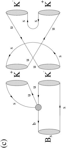
Figure 2: Examples of rescattering processes contributing to $B_{s}\to K\overline{K}$. The shaded circles represent insertions of the usual current–current operators $Q_{1,2}^{u}$, and $q\in\{u,d\}$ distinguishes between the final states $K^{+}K^{-}$ and $K^{0}\overline{K^{0}}$. The annihilation-like topology (c) arises only in the case of $B^{0}_{s}\to K^{+}K^{-}$ and contributes to the amplitude $\tilde{\cal E}_{s}$.

As was pointed out in [17, 33], the usual argument for the suppression of annihilation processes relative to tree-diagram-like topologies by a factor $f_{B}/m_{B}$ does not apply to rescattering processes. Consequently, these topologies may also play a more important role than naïvely expected. Model calculations [33] based on Regge phenomenology typically give an enhancement of the ratio $|{\cal A}|/|\tilde{\cal T}|$ from $f_{B}/m_{B}\approx 0.04$ to ${\cal O}(0.2)$. Rescattering processes of this kind can be probed, e.g. by the $\Delta S$ = 0 decay $B^{0}_{d}\to K^{+}K^{-}$. A future stringent bound on BR$(B^{0}_{d}\to K^{+}K^{-})$ at the level of $10^{-7}$ or lower may provide a useful limit on these rescattering effects [6]. The present upper bound obtained by the CLEO collaboration is $4.3\times 10^{-6}$ [9].

In the case of $B_{s}\to K\overline{K}$ decays, we have to deal with final-state interaction effects related to rescattering processes such as $B_{s}\to\{K^{+}K^{-}\}\to K^{0}\overline{K^{0}}$, which are illustrated in Fig. 2. Here the shaded circles represent insertions of the current–current operators

$$Q_{1}^{u}=(\bar{u}_{\alpha}s_{\beta})_{{\rm V-A}}\;(\bar{b}_{\beta}u_{\alpha})_{{\rm V-A}}\,,\quad Q_{2}^{u}=(\bar{u}_{\alpha}s_{\alpha})_{{\rm V-A}}\;(\bar{b}_{\beta}u_{\beta})_{{\rm V-A}}\,,$$ (56)

where $\alpha$ and $\beta$ are $SU(3)_{\rm C}$ colour indices. The topologies of the kind (a) and (b) shown in this figure contribute both to $\rho_{s}\,e^{i\theta_{s}}$ (see (18)), while (c) represents a potentially important contribution to the “exchange” amplitude $\tilde{\cal E}_{s}$, arising in the case of $B_{s}\to K^{+}K^{-}$. Topologies of the latter kind describe also contributions to the “penguin annihilation” amplitudes $(PA)_{s}$, if the current–current operators are replaced by penguin operators.

Although specific model calculations of these $B_{s}$ rescattering processes have not yet been performed, it is plausible to assume that features similar to those occurring for their $B_{u,d}$ counterparts may show up. Consequently, $\rho_{s}$ may be as large as ${\cal O}(10\%)$, and the role of the exchange and penguin annihilation amplitudes may be underestimated by the naïve expectation $|\tilde{\cal E}_{s}|/|\tilde{\cal T}_{s}|\approx|(PA)_{s}|/|P_{s}|\approx 0.04$. An important experimental tool to investigate the latter feature is provided by the transition $B_{s}\to\pi^{+}\pi^{-}$, which exhibits a decay amplitude proportional to $\tilde{\cal E}_{s}+(PA)_{s}$. The naïve expectation for the corresponding branching ratio is ${\cal O}(10^{-8})$, and a significant enhancement would indicate that rescattering contributions, as those shown in Fig. 2 (c), play an important role.

If we look at the untagged $B_{s}\to K^{0}\overline{K^{0}}$ rate (31) and their observables (34) and (35), we notice that the term proportional to $R_{H}$, evolving in time with the decay width $\Gamma_{H}^{(s)}$, is essentially due to rescattering processes. In Fig. 3, we illustrate this feature, which has some analogy to the generation of the CP asymmetry $A_{+}$ arising in $B^{\pm}\to\pi^{\pm}K$, by showing the dependence of the ratio $R_{H}/R_{L}$ on the CKM angle $\gamma$ for various values of $\rho_{s}$ and $\theta_{s}\in\{0^{\circ},180^{\circ}\}$. Since $R_{H}$ is proportional to $\rho_{s}^{2}$, final-state interaction effects may lead to values of $R_{H}/R_{L}$ of at most ${\cal O}(10\%)$. Consequently, a measurement of the part of the untagged $B_{s}\to K^{0}\overline{K^{0}}$ rate proportional to $e^{-\Gamma_{H}^{(s)}t}$ may be very difficult. However, as we will see in Section 7, the ratio $R_{H}/R_{L}$ could be dramatically enhanced from this Standard Model expectation, if $B^{0}_{s}$–$\overline{B^{0}_{s}}$ mixing receives sizeable CP-violating contributions from new physics.

Figure 3: The dependence of the ratio $R_{H}/R_{L}$ of the $B_{s}\to K^{0}\overline{K^{0}}$ observables on the CKM angle $\gamma$ for various values of $\rho_{s}$ and $\theta_{s}\in\{0^{\circ},180^{\circ}\}$.

Figure 4: The constraints on the parameter $\rho_{s}$ arising from the observables $R_{H}$ and $R_{L}$ of the untagged $B_{s}\to K^{0}\overline{K^{0}}$ rate.

In the case of the decay $B^{+}\to\pi^{+}K^{0}$, the CP asymmetry $A_{+}$ implies upper and lower bounds for $\rho$, which are given by

$$\rho_{\rm min}^{\rm max}=\frac{\sqrt{A_{+}^{2}\,+\,\left(1-A_{+}^{2}\right)\sin^{2}\gamma}\,\pm\,\sqrt{\left(1-A_{+}^{2}\right)\sin^{2}\gamma}}{|A_{+}|}\,,$$ (57)

and are discussed in detail in [8]. Concerning the mode $B_{s}\to K^{0}\overline{K^{0}}$, the ratio of the observables $R_{H}$ and $R_{L}$ implies upper and lower bounds for $\rho_{s}$, which take the form

$$(\rho_{s})^{\rm max}_{\rm min}=\frac{\sqrt{R_{H}}}{\left|\sqrt{R_{L}}\,|\sin\gamma|\,\mp\,\sqrt{R_{H}}\,|\cos\gamma|\right|}\,,$$ (58)

and are very different from (57). In Fig. 4, we show the dependence of (58) on the CKM angle $\gamma$ for various values of $R_{H}/R_{L}$. Interestingly, we have $(\rho_{s})_{\rm min}=(\rho_{s})^{\rm max}=\sqrt{R_{H}/R_{L}}$ for $\gamma=90^{\circ}$, so that $\rho_{s}$ is fixed completely in this case. The corresponding CP-conserving strong phases $(\theta_{s})^{\rm max}_{\rm min}$ are given by

$$(\theta_{s})_{\rm min}=\left\{\begin{array}[]{lcl}180^{\circ}&\,\mbox{for}&0^{\circ}<\gamma<90^{\circ}\\ 0^{\circ}&\,\mbox{for}&90^{\circ}<\gamma<180^{\circ}\end{array}\right\},\,\,\,(\theta_{s})^{\rm max}=\left\{\begin{array}[]{lcl}0^{\circ}&\,\mbox{for}&0^{\circ}<\gamma<90^{\circ}\\ 180^{\circ}&\,\mbox{for}&90^{\circ}<\gamma<180^{\circ}\end{array}\right\}$$ (59)

for $|\tan\gamma|>\sqrt{R_{H}/R_{L}}$, and by $(\theta_{s})^{\rm max}=(\theta_{s})_{\rm min}$ with $(\theta_{s})_{\rm min}$ given in (59) otherwise.

In order to constrain the CKM angle $\gamma$ in the presence of rescattering effects, i.e. $\rho_{s}\not=0$, we follow the strategy discussed in Subsection 3.2 and eliminate $r_{s}$ in (2.2) through (46), which yields the equation

$$A_{\rho}\,\cos^{2}\delta_{s}\,+\,2\,B_{\rho}\,\cos\delta_{s}\,\sin\delta_{s}\,-\,C^{2}_{\rho}\,=\,0\,,$$ (60)

having the solution

$$\cos^{2}\delta_{s}=\frac{A_{\rho}\,C^{2}_{\rho}\,+\,2\,B^{2}_{\rho}\,\pm\,2\,B_{\rho}\,\sqrt{A_{\rho}\,C^{2}_{\rho}\,+\,B^{2}_{\rho}\,-\,C^{4}_{\rho}}}{A^{2}_{\rho}\,+\,4\,B_{\rho}^{2}}$$ (61)

with

$$A_{\rho} = \frac{4}{w_{s}^{2}}\left[\left(\frac{b}{\sin^{2}\gamma}\right)\,-\,\frac{\rho_{s}^{2}}{w_{s}^{2}}\right]\cos^{2}\gamma\,+\,4\,C_{\rho}\frac{\rho_{s}}{w_{s}^{2}}\cos\theta_{s}\,\cos\gamma$$ (62)

$$B_{\rho} = 2\,C_{\rho}\,\frac{\rho_{s}}{w_{s}^{2}}\,\sin\theta_{s}\,\cos\gamma$$ (63)

$$C_{\rho} = 1\,-\,a\,+\,b\left(\frac{\cos\gamma}{\sin\gamma}\right)^{2}-\,\frac{\rho_{s}^{2}}{w_{s}^{2}}\,.$$ (64)

In these expressions, which represent the generalization of (47) in the presence of rescattering processes, electroweak penguin effects have been neglected, i.e. $\epsilon_{s}=0$. The corresponding contours in the $\gamma\,$–$\,\cos\delta_{s}$ plane are shown in Fig. 5 for $\rho_{s}=0.15$, various values of the strong phase $\theta_{s}$, and the $B_{s}\to K^{+}K^{-}$ observables $(a,b)=(0.60,0.15)$ and $(1.40,0.15)$. The thick solid lines represent the curves shown in Fig. 1. We observe that the final-state interaction effects are negligible in the case of $\theta_{s}=\pm\,90^{\circ}$, and are maximal for $\theta_{s}\in\{0^{\circ},180^{\circ}\}$, leading to an uncertainty of $\Delta\gamma=\pm\,8^{\circ}$ in this specific example.

Figure 5: The contours in the $\gamma\,$–$\,\cos\delta_{s}$ plane corresponding to $(a,b)=(0.60,0.15)$ and $(1.40,0.15)$ in the presence of rescattering effects described by $\rho_{s}=0.15$.

Figure 6: The contours in the $\gamma\,$–$\,\cos\delta_{s}$ plane corresponding to $(\rho_{s})^{\rm max}_{\rm min}$ for $R_{H}/R_{L}=0.025$ and $(a,b)=(0.60,0.15)$, $(1.40,0.15)$.

If it were possible to measure the ratio $R_{H}/R_{L}$ of the observables of the untagged $B_{s}\to K^{0}\overline{K^{0}}$ decay rate, either $\theta_{s}$ or $\rho_{s}$ could be eliminated in (62)–(64), and the quantity $w_{s}$ defined by (41) could be fixed through

$$w_{s}=\rho_{s}\,\sqrt{1+\frac{R_{L}}{R_{H}}}\,|\sin\gamma|\,.$$ (65)

The upper and lower bounds for $\rho_{s}$ that are implied by $R_{H}/R_{L}$ also play an important role to constrain the rescattering effects in the $\gamma\,$–$\,\cos\delta_{s}$ plane. If we assume, for illustrative purposes, that $R_{H}/R_{L}=0.025$ has been measured, and insert (58) and (59) in (62)–(64), we obtain the curves shown in Fig. 6, demonstrating nicely the way in which the final-state interaction effects can be controlled. By the time the $B_{s}\to K\overline{K}$ observables can be measured, we will probably have deeper insights into rescattering processes from analyses of $B^{\pm}\to K^{\pm}K$ and $B^{\pm}\to\pi^{\pm}K$ modes anyway, which – making use of the strategies proposed in [8, 20] – may provide stringent constraints on the parameter $\rho$.

4.2 The Role of Electroweak Penguins

In order to investigate the impact of electroweak penguins on the constraints on the CKM angle $\gamma$ arising from untagged $B_{s}\to K\overline{K}$ decays, let us neglect the rescattering effects discussed in the previous subsection. Combining (2.2) and (40), we obtain

$$H_{\epsilon}\,\cos\delta_{s}\,+\,K_{\epsilon}\,\sin\delta_{s}=M_{\epsilon}$$ (66)

with

$$H_{\epsilon}\,=\,1\,+\,\epsilon_{s}\,\cos\Delta_{s}\,,\quad K_{\epsilon}\,=\,\epsilon_{s}\,\sin\Delta_{s}\,,$$ (67)

$$M_{\epsilon}\,=\,\frac{|\sin\gamma|}{2\,\sqrt{b}\,\cos\gamma}\left[1\,+\,2\,\epsilon_{s}\cos\Delta_{s}\,+\,\epsilon_{s}^{2}\,-\,a\,+\,b\left(\frac{\cos\gamma}{\sin\gamma}\right)^{2}\right],$$ (68)

yielding

$$\cos\delta_{s}=\frac{H_{\epsilon}\,M_{\epsilon}\,\pm\,K_{\epsilon}\,\sqrt{H_{\epsilon}^{2}+K_{\epsilon}^{2}-M_{\epsilon}^{2}}}{H_{\epsilon}^{2}+K_{\epsilon}^{2}}\,.$$ (69)

The corresponding contours in the $\gamma\,$–$\,\cos\delta_{s}$ plane are illustrated in Fig. 7 for the $B_{s}\to K^{+}K^{-}$ observables $(a,b)=(0.60,0.15)$ and $(1.40,0.15)$, $\epsilon_{s}=0.1$, and various values of the strong phase difference $\Delta_{s}$. These curves are similar to those shown in Fig. 5 describing the final-state interaction effects. The electroweak penguin effects are negligibly small for $\Delta_{s}=\pm\,90^{\circ}$, and maximal for $\Delta_{s}\in\{0^{\circ},180^{\circ}\}$, leading to an uncertainty of $\Delta\gamma=\pm\,11^{\circ}$ in this example.

Figure 7: The contours in the $\gamma\,$–$\,\cos\delta_{s}$ plane corresponding to $(a,b)=(0.60,0.15)$ and $(1.40,0.15)$ in the presence of electroweak penguins described by $\epsilon_{s}=0.1$.

Figure 8: The contours in the $\gamma\,$–$\,\cos\delta_{s}$ plane corresponding to $(a,b)=(0.60,0.15)$ and $(1.40,0.15)$ in the presence of electroweak penguins described by $a_{s}=0.25$.

In the case of $B_{u,d}\to\pi K$ and $B_{s}\to K\overline{K}$ decays, electroweak penguins contribute only in “colour-suppressed” form; estimates based on simple calculations performed at the perturbative quark level, where the relevant hadronic matrix elements are treated within the “factorization” approach, typically give $\epsilon_{(s)}={\cal O}(1\%)$ [5]. Since these crude estimates may, however, well underestimate the role of electroweak penguins [6, 17, 32], we have used $\epsilon_{s}=0.1$ in Fig. 7. Consequently, an improved theoretical description of electroweak penguins is highly desirable. In Ref. [8], the expressions of the electroweak penguin operators and the isospin symmetry of strong interactions have been used to derive the following expression:

$$\frac{\epsilon}{r}\,e^{i(\Delta-\delta)}\approx 0.75\times a_{u,d}\,e^{i\omega_{u,d}}\,,$$ (70)

where

$$a_{u,d}\,e^{i\omega_{u,d}}\equiv\frac{a_{2}^{\rm eff}}{a_{1}^{\rm eff}}$$ (71)

is the ratio of generalized, complex colour factors corresponding to the usual coefficients $a_{1}$ and $a_{2}$. A similar relation holds also for the $B_{s}\to K\overline{K}$ parameters. Consequently, we have

$$\epsilon_{s}=q_{s}\,r_{s}\,,\quad\Delta_{s}=\delta_{s}+\omega_{s}$$ (72)

with $q_{s}\approx 0.75\times a_{s}$. Using (72), the definitions (67) and (68) are modified as follows:

$$H_{\epsilon}\,\to\,H_{q}\,=\,\cos\gamma\,-\,q_{s}\,\cos\omega_{s}\,,\quad K_{\epsilon}\,\to\,K_{q}\,=\,q_{s}\,\sin\omega_{s}\,,$$ (73)

$$M_{\epsilon}\,\to\,M_{q}\,=\,\frac{|\sin\gamma|}{2\,\sqrt{b}}\left[1\,-\,a\,+\,\frac{b}{\sin^{2}\gamma}\left(\cos^{2}\gamma\,-\,2\,q_{s}\cos\omega_{s}\,\cos\gamma\,+\,q_{s}^{2}\right)\right].$$ (74)

In Fig. 8, we show the corresponding contours in the $\gamma\,$–$\,\cos\delta_{s}$ plane for the same observables $a$ and $b$ as in our previous examples, $a_{s}=0.25$, and various values of the CP-conserving strong phase $\omega_{s}$. A first step towards constraining the electroweak penguin contributions experimentally is provided by the mode $B^{+}\to\pi^{+}\pi^{0}$, and is closely related to the issue of “colour-suppression”, as discussed in detail in [8].

4.3 Combined Rescattering and Electroweak Penguin Effects

The formulae describing combined rescattering and electroweak penguin effects in the contours in the $\gamma\,$–$\,\cos\delta_{s}$ plane are rather complicated. Eliminating $r_{s}$ in (2.2) through (46) yields an equation to determine $\cos\delta_{s}$, which has a form similar to (60):

$$\tilde{A}\,\cos^{2}\delta_{s}\,+\,2\,\tilde{B}\,\cos\delta_{s}\,\sin\delta_{s}\,-\,\tilde{C}\,=\,0,$$ (75)

and the solution

$$\cos^{2}\delta_{s}=\frac{\tilde{A}\,\tilde{C}\,+\,2\,\tilde{B}^{2}\,\pm\,2\,\tilde{B}\,\sqrt{\tilde{A}\,\tilde{C}\,+\,\tilde{B}^{2}\,-\,\tilde{C}^{2}}}{\tilde{A}^{2}\,+\,4\,\tilde{B}^{2}}\,.$$ (76)

The quantities $\tilde{A}$, $\tilde{B}$ and $\tilde{C}$ are given by

$$\tilde{A} = \left(\tilde{h}^{2}\,-\,\tilde{k}^{2}\right)\tilde{D}\,+\,4\,\tilde{E}\,\frac{\rho_{s}}{w_{s}^{2}}\left(\tilde{h}\,\cos\theta_{s}\,-\,\tilde{k}\,\sin\theta_{s}\right)\cos\gamma$$ (77)

$$\tilde{B} = \tilde{h}\,\tilde{k}\,\tilde{D}\,+\,2\,\tilde{E}\,\frac{\rho_{s}}{w_{s}^{2}}\left(\tilde{k}\,\cos\theta_{s}\,+\,\tilde{h}\,\sin\theta_{s}\right)\cos\gamma$$ (78)

$$\tilde{C} = \tilde{E}^{2}\,-\,4\,\tilde{E}\,\frac{\rho_{s}}{w_{s}^{2}}\,\tilde{k}\,\sin\theta_{s}\,\cos\gamma\,-\,\tilde{k}^{2}\tilde{D}$$ (79)

with

$$\tilde{h}=1\,+\,\epsilon_{s}\,w_{s}\,\cos\Delta_{s}\,,\quad\tilde{k}=\epsilon_{s}\,w_{s}\,\sin\Delta_{s}$$ (80)

and

$$\tilde{D} = \frac{4}{w^{2}_{s}}\left[\left(\frac{b}{\sin^{2}\gamma}\right)\,-\,\frac{\rho_{s}^{2}}{w_{s}^{2}}\right]\cos^{2}\gamma$$ (81)

$$\tilde{E} = 1-a+b\left(\frac{\cos\gamma}{\sin\gamma}\right)^{2}-\,\frac{\rho_{s}^{2}}{w_{s}^{2}}+2\,\frac{\epsilon_{s}}{w_{s}}\,\biggl{[}\cos\Delta_{s}+\rho_{s}\,\cos(\Delta_{s}-\theta_{s})\,\cos\gamma\biggr{]}+\,\epsilon_{s}^{2}\,.$$ (82)

In order to derive these expressions, no approximations have been made and they are valid exactly.

5 Combining $B_{u,d}\to\pi K$ and Untagged $B_{s}\to K\overline{K}$ Decays Through $SU(3)$ Flavour Symmetry

So far, we have discussed the $B_{u,d}\to\pi K$ and $B_{s}\to K\overline{K}$ decays separately. As we have just seen, interesting constraints on $\gamma$ may arise from the corresponding observables. The goal is, however, not only to constrain, but eventually to determine $\gamma$. If we consider the modes $B_{u,d}\to\pi K$ and $B_{s}\to K\overline{K}$ separately, information about the magnitudes of the amplitudes $T$ and $T_{s}$ is needed to accomplish this task [4, 6, 24]. Such an input can be avoided, if the $SU(3)$ flavour symmetry of strong interactions is applied, yielding

$$\cos\delta_{s}=\zeta_{\delta}\,\cos\delta\,,\quad r_{s}=\zeta_{r}\,r\,,$$ (83)

where the quantities $\zeta_{\delta}$ and $\zeta_{r}$ parametrize $SU(3)$-breaking corrections. As a first “guess”, we may use $\zeta_{\delta}=1$, $\zeta_{r}=1$, which corresponds to the strict $SU(3)$ limit. In order to extract $\gamma$ from a simultaneous analysis of $B_{u,d}\to\pi K$ and $B_{s}\to K\overline{K}$ decays, each of the two expressions given in (83) is in principle sufficient. The former applies to the contours in the $\gamma\,$–$\,\cos\delta_{(s)}$ plane, while the latter can be used for the $\gamma\,$–$\,r_{(s)}$ plane.

Let us first turn to the contours in the $\gamma\,$–$\,\cos\delta_{(s)}$ plane. In the case of the $B_{s}\to K\overline{K}$ decays, these contours play a key role to constrain the CKM angle $\gamma$, while it is more “natural” to consider contours in the $\gamma\,$–$\,r$ plane in the case of the $B_{u,d}\to\pi K$ modes [8]. However, the $B_{u,d}\to\pi K$ observables $R$ and $A_{0}$ fix also contours in the $\gamma\,$–$\,\cos\delta$ plane. If we eliminate $r$ in $R$ through the “pseudo-asymmetry” $A_{0}$ (see (21) and (22)), we obtain

$$\cos^{2}\delta\,=\,\frac{2\,V^{2}\,-\,U\,W\,\pm\,2\,V\,\sqrt{V^{2}\,-\,U\,W\,-\,W^{2}}}{U^{2}\,+\,4\,V^{2}}$$ (84)

with

$$U = 2\,A\left(k\,B\,+\,h\,C\,\right)\,+\,\left(B^{2}\,-\,C^{2}\right)\left(R\,-\,R_{0}\right)$$ (85)

$$V = B\,C\left(R\,-\,R_{0}\right)\,-\,A\left(h\,B\,-\,k\,C\right)$$ (86)

$$W = A^{2}\,-\,2\,k\,A\,B\,-\,\left(R\,-\,R_{0}\right)B^{2}\,,$$ (87)

where the quantities

$$h=\frac{1}{w}\left(\cos\gamma+\rho\,\cos\theta\right)+\epsilon\,\cos\Delta\,\cos\gamma\,,\quad k=\frac{\rho}{w}\,\sin\theta+\epsilon\,\sin\Delta\,\cos\gamma$$ (88)

$$A=\frac{A_{0}-A_{+}}{2\,\sin\gamma}-\frac{\epsilon\,\rho}{w}\,\sin(\Delta-\theta)\,,\quad B=\frac{1}{w}+\epsilon\,\cos\Delta\,,\quad C=\epsilon\,\sin\Delta\,,$$ (89)

and

$$R_{0}=1+2\,\frac{\epsilon}{w}\,\left[\,\cos\Delta+\rho\,\cos(\Delta-\theta)\cos\gamma\,\right]+\epsilon^{2}$$ (90)

were introduced in [8]. The corresponding contours in the $\gamma\,$–$\,\cos\delta$ plane are illustrated in Fig. 9 for $R=0.65$, $1.05$, and various values of $A_{0}$ in the case of neglected rescattering and electroweak penguin effects. Using the formulae given above and the strategies proposed in [8, 20], these effects can be included in these contours. For $R=0.65$, a significant range around $\gamma=90^{\circ}$ is excluded, which corresponds to $R<R_{\rm min}$, where $R_{\rm min}$ is given in (44). If the contours arising in the $\gamma\,$–$\,\cos\delta_{s}$ plane determined from the untagged $B_{s}\to K\overline{K}$ decays are included in the same figure (see Fig. 1), $\gamma$ and $\cos\delta_{(s)}$ can be determined with the help of the first relation given in (83).

Another approach to accomplish this task is to consider the contours in the $\gamma\,$–$\,r_{(s)}$ plane. To this end, we rewrite the observable $a$ given in (2.2) as

$$a=a_{0}\,-\,2\,r_{s}\left(f\,\cos\delta_{s}\,+\,g\,\sin\delta_{s}\right)\,+\,r_{s}^{2}\cos^{2}\gamma$$ (91)

with

$$a_{0}=1+2\,\frac{\epsilon_{s}}{w_{s}}\left[\cos\Delta_{s}+\rho_{s}\,\cos(\Delta_{s}-\theta_{s})\,\cos\gamma\right]+\epsilon_{s}^{2}-\frac{\rho_{s}^{2}}{w_{s}^{2}}\,\sin^{2}\gamma$$ (92)

$$f=\left[\frac{1}{w_{s}}\left(1+\rho_{s}\cos\theta_{s}\cos\gamma\right)+\epsilon_{s}\cos\Delta_{s}\right]\cos\gamma,\,\,\,g=\left(\frac{\rho_{s}}{w_{s}}\sin\theta_{s}\cos\gamma+\epsilon_{s}\sin\Delta_{s}\right)\cos\gamma,$$ (93)

and eliminate the strong phase $\delta_{s}$ in (40), yielding

$$r_{s}=\sqrt{S\,\pm\,\sqrt{S^{2}\,-\,T}}\,,$$ (94)

where

$$S=\frac{p\,q+l^{2}\,m}{q^{2}+l^{2}\cos^{4}\gamma}\,,\quad T=\frac{p^{2}+(a-a_{0})^{2}\,l^{2}}{q^{2}+l^{2}\cos^{4}\gamma}$$ (95)

with

$$p = \frac{b}{\sin^{2}\gamma}-\frac{\rho_{s}^{2}}{w_{s}^{2}}-\frac{\rho_{s}}{w_{s}}\,(a-a_{0})\left(\frac{f\cos\theta_{s}+g\,\sin\theta_{s}}{f^{2}+g^{2}}\right)$$ (96)

$$q = 1-\frac{\rho_{s}}{w_{s}}\left(\frac{f\cos\theta_{s}+g\,\sin\theta_{s}}{f^{2}+g^{2}}\right)\cos^{2}\gamma$$ (97)

$$l = \frac{\rho_{s}}{w_{s}}\left(\frac{g\,\cos\theta_{s}-f\sin\theta_{s}}{f^{2}+g^{2}}\right)$$ (98)

$$m = 2\,(f^{2}+g^{2})+(a-a_{0})\cos^{2}\gamma\,.$$ (99)

Figure 9: The contours in the $\gamma\,$–$\,\cos\delta$ plane for $R=0.65$, $1.05$ and various values of $A_{0}$ in the case of neglected rescattering and electroweak penguin effects.

Figure 10: The contours in the $\gamma\,$–$\,r_{s}$ plane for $a=0.60$, $b=0.15$ and $\rho_{s}=0.15$, $\epsilon_{s}=0$. The $B_{u,d}\to\pi K$ contours correspond to $R=0.75$, $A_{0}=0.2$ and $\rho=\epsilon=0$.

In Fig. 10, we have illustrated the corresponding contours in the $\gamma\,$–$\,r_{s}$ plane by choosing $a=0.60$ and $b=0.15$. The thick solid line has been calculated for $\rho_{s}=0$, while the thin lines have been obtained for $\rho_{s}=0.15$ and various values of the strong phase $\theta_{s}$. The effects of electroweak penguins have been neglected in this figure. Since the observable $b$ is not affected by electroweak penguins at all, as can be seen in (40), their effect on the contours in the $\gamma\,$–$\,r_{s}$ plane is rather small and is only due to the elimination of $\delta_{s}$ through the observable $a$. In Fig. 10, we have also included the contours arising from the $B_{u,d}\to\pi K$ observables $R=0.75$ and $A_{0}=0.2$ in the case of $\zeta_{r}=1$ and neglected rescattering and electroweak penguin effects, which can be taken into account by using the strategies presented in [8, 20]. Combining the $B_{s}\to K\overline{K}$ and $B_{u,d}\to\pi K$ contours, $\gamma$ and $r_{(s)}$ can be determined, as illustrated in Fig. 10. The $SU(3)$-breaking parameter $\zeta_{r}$ can be expressed as

$$\zeta_{r}=\sqrt{\frac{\left\langle|P|^{2}\right\rangle}{\left\langle|P_{s}|^{2}\right\rangle}}\frac{|T_{s}|}{|T|}\,,$$ (100)

where $\left\langle|P|^{2}\right\rangle$ and $\left\langle|P_{s}|^{2}\right\rangle$ can be fixed experimentally through the combined $B^{\pm}\to\pi^{\pm}K$ branching ratio (2) and the untagged $B_{s}\to K^{0}\overline{K^{0}}$ rate (37), respectively. Comparing their values with those of $R$ and $R_{s}$, we obtain interesting insights into $SU(3)$ breaking. The amplitudes $T$ and $T_{s}$ are given in (14) and (2.1), respectively, and their structure is quite similar. Note that the different signs of the ${\cal A}$ and $\tilde{\cal E}$ contributions are only due to our definition of meson states (see, for instance, [28]). In the strict $SU(3)$ limit, the combinations $\tilde{\cal T}-{\cal A}$ and $\tilde{\cal T}_{s}+\tilde{\cal E}_{s}$ would be equal.

Assuming $|T|\approx|T_{s}|$ is probably more reliable than $\cos\delta_{s}\approx\cos\delta$. However, as soon as the $B_{u,d}\to\pi K$ observables $R$ and $A_{0}$, as well as the $B_{s}\to K\overline{K}$ observables $a$ and $b$ have been measured, both the contours in the $\gamma\,$–$\,r_{(s)}$ plane and those in the $\gamma\,$–$\,\cos\delta_{(s)}$ plane should be considered to extract the CKM angle $\gamma$ and the hadronic parameters $r_{(s)}$ and $\cos\delta_{(s)}$ as discussed above. In addition to $\gamma$, in particular $r_{(s)}$ would be of special interest, since it allows a test of the factorization hypothesis by comparing its experimentally determined value with (43).

Figure 11: Representation of the amplitude relations (16) and (17) between the decays $B_{s}^{0}\to K^{+}K^{-}$, $B_{s}^{0}\to K^{0}\overline{K^{0}}$ and their charge conjugates in the complex plane.

6 A Brief Look at a Tagged Analysis of $B_{s}\to K\overline{K}$

In this paper, we have so far focused on the observables provided by an untagged measurement of the decays $B_{s}\to K^{0}\overline{K^{0}}$ and $B_{s}\to K^{+}K^{-}$, where the rapid oscillatory $\Delta M_{s}t$-terms cancel. Let us briefly discuss, in this section, an interesting feature of a tagged analysis of these modes. If the $\Delta M_{s}t$-oscillations could be resolved in such a measurement, the CKM angle $\gamma$ could be extracted by using only the amplitude relations (16) and (17), which are based on the $SU(2)$ isospin symmetry of strong interactions and are completely general. These relations can be represented in the complex plane as triangles for the $B_{s}^{0}\to K\overline{K}$ decays and their charge conjugates, as shown in Fig. 11, where $A_{s}\equiv A(B^{0}_{s}\to K^{+}K^{-})$, $P_{s}\equiv A(B^{0}_{s}\to K^{0}\overline{K^{0}})$, and $t_{s}\equiv T_{s}+P_{\rm ew}^{s}$. The angles $\varphi$ and $\psi$ can be determined by measuring the time-dependent CP asymmetries arising in $B^{0}_{s}\to K^{+}K^{-}$ and $B^{0}_{s}\to K^{0}\overline{K^{0}}$. These CP-violating asymmetries are defined for a generic final state $f$ by

$$a_{\rm CP}(t;f)\equiv\frac{\Gamma(B_{s}^{0}(t)\to f)\,-\,\Gamma(\overline{B^{0}_{s}}(t)\to f)}{\Gamma(B_{s}^{0}(t)\to f)\,+\,\Gamma(\overline{B^{0}_{s}}(t)\to f)}\,.$$ (101)

If $f$ is a CP eigenstate, we have

$$a_{\rm CP}(t;f)=2\,e^{-\Gamma_{s}t}\left[\frac{{\cal A}_{\rm CP}^{\rm dir}(B_{s}\to f)\cos(\Delta M_{s}t)+{\cal A}_{\rm CP}^{\rm mix-ind}(B_{s}\to f)\sin(\Delta M_{s}t)}{e^{-\Gamma_{H}^{(s)}t}+e^{-\Gamma_{L}^{(s)}t}\,+\,{\cal A}_{\Delta\Gamma}(B_{s}\to f)\left(e^{-\Gamma_{H}^{(s)}t}\,-\,e^{-\Gamma_{L}^{(s)}t}\right)}\right],$$ (102)

where

$${\cal A}_{\rm CP}^{\rm dir}(B_{s}\to f)=\frac{1-\left|\xi_{f}\right|^{2}}{1+\left|\xi_{f}\right|^{2}}\,,\quad{\cal A}_{\rm CP}^{\rm mix-ind}(B_{s}\to f)=\frac{2\,\mbox{Im}(\xi_{f})}{1+\left|\xi_{f}\right|^{2}}\,,$$ (103)

and

$${\cal A}_{\Delta\Gamma}(B_{s}\to f)=\frac{2\,\mbox{Re}(\xi_{f})}{1+\left|\xi_{f}\right|^{2}}$$ (104)

can be determined straightforwardly from the untagged rate given in (29). The observable $\xi_{f}$ has been introduced in (30). In the case of the decays $B_{s}\to K^{+}K^{-}$ and $B_{s}\to K^{0}\overline{K^{0}}$, we have

$${\cal A}_{\rm CP}^{\rm dir}(B_{s}\to K^{+}K^{-}) = \frac{|A_{s}|^{2}-|\overline{A_{s}}|^{2}}{|A_{s}|^{2}+|\overline{A_{s}}|^{2}}$$ (105)

$${\cal A}_{\rm CP}^{\rm mix-ind}(B_{s}\to K^{+}K^{-}) = \frac{2\,|A_{s}||\overline{A_{s}}|}{|A_{s}|^{2}+|\overline{A_{s}}|^{2}}\,\sin\left(\phi_{\rm M}^{(s)}+\varphi\right)$$ (106)

and

$${\cal A}_{\rm CP}^{\rm dir}(B_{s}\to K^{0}\overline{K^{0}}) = \frac{|P_{s}|^{2}-|\overline{P_{s}}|^{2}}{|P_{s}|^{2}+|\overline{P_{s}}|^{2}}$$ (107)

$${\cal A}_{\rm CP}^{\rm mix-ind}(B_{s}\to K^{0}\overline{K^{0}}) = \frac{2\,|P_{s}||\overline{P_{s}}|}{|P_{s}|^{2}+|\overline{P_{s}}|^{2}}\,\sin\left(\phi_{\rm M}^{(s)}+\psi\right),$$ (108)

where $\phi_{\rm M}^{(s)}=0$ to a good approximation in the Standard Model. The observables ${\cal A}_{\Delta\Gamma}(B_{s}\to K^{+}K^{-})$ and ${\cal A}_{\Delta\Gamma}(B_{s}\to K^{0}\overline{K^{0}})$ probe $\cos\left(\phi_{\rm M}^{(s)}+\varphi\right)$ and $\cos\left(\phi_{\rm M}^{(s)}+\psi\right)$, respectively. Consequently, the CP-violating observables allow the construction of the amplitudes $A_{s}$, $\overline{A_{s}}$ and $P_{s}$, $\overline{P_{s}}$ in the complex plane, i.e. of the dashed and solid lines in Fig. 11 (a). So far, we have not made any approximations, and this construction is valid exactly. However, in order to extract $\gamma$, we have to neglect the electroweak penguin amplitude $P_{\rm ew}^{s}$. Then we have $t_{s}=T_{s}$, and the relative orientation of the $A_{s}$, $P_{s}$, $T_{s}$ and $\overline{A_{s}}$, $\overline{P_{s}}$, $\overline{T_{s}}$ amplitudes can be fixed by requiring $|T_{s}|=|\overline{T_{s}}|$. The angle between $T_{s}$ and $\overline{T_{s}}$ is given by $2\gamma$. In Fig. 11 (b), the impact of electroweak penguins on this construction is illustrated for $\omega_{s}=0^{\circ}$ (see (72)).

From a conceptual point of view, this determination of $\gamma$ is quite analogous to that of the extraction of the CKM angle $\alpha$ from a combined analysis of the decays $B_{d}\to\pi^{+}\pi^{-}$ and $B_{d}\to K^{0}\overline{K^{0}}$, which was proposed in [34]. Recently, a study of tagged $B_{s}\to K^{0}\overline{K^{0}}$ and $B_{s}\to K^{+}K^{-}$ decays was performed in [35], where also the possibility of extracting $\gamma$ from these decays was pointed out. However, in that paper rescattering and electroweak penguin effects were neglected. Here we have shown that a time-dependent analysis of tagged $B_{s}\to K\overline{K}$ decays allows a determination of $\gamma$ taking into account rescattering effects “automatically”. This approach works also if new physics contributes to $B^{0}_{s}$–$\overline{B^{0}_{s}}$ mixing.

7 Physics Beyond the Standard Model

Let us focus in this section on a particular scenario of new physics [36, 37], where the $B_{u,d}\to\pi K$ and $B_{s}\to K\overline{K}$ modes are governed by the Standard Model diagrams and $B^{0}_{s}$–$\overline{B^{0}_{s}}$ mixing receives significant CP-violating new-physics contributions. A similar scenario for the $B_{u,d}\to\pi K$ modes and $B^{0}_{d}$–$\overline{B^{0}_{d}}$ mixing was considered in [15]. While the CP-violating weak mixing phase of the $B_{s}$ system vanishes to a good approximation within the Standard Model, as we have already noted, new physics may lead to a sizeable CP-violating weak $B^{0}_{s}$–$\overline{B^{0}_{s}}$ mixing phase. Applying the same notation as in [3, 37], we have

$$\phi_{\rm M}^{(s)}=0+2\,\phi_{\rm new}^{(s)}\equiv 2\,\phi\,.$$ (109)

If the decay $B_{s}\to K^{0}\overline{K^{0}}$ is still dominated by the Standard Model contributions, the observables $R_{L}$ and $R_{H}$ of the corresponding untagged transition rate introduced in (34) and (35) are modified as follows:

$$R_{L}=\left[\cos^{2}\phi+2\,\rho_{s}\cos\theta_{s}\cos\phi\cos\left(\phi+\gamma\right)+\rho_{s}^{2}\cos^{2}\left(\phi+\gamma\right)\right]\Gamma_{0}$$ (110)

$$R_{H}=\left[\,\sin^{2}\phi\,+\,2\,\rho_{s}\cos\theta_{s}\sin\phi\sin\left(\phi+\gamma\right)+\rho_{s}^{2}\sin^{2}\left(\phi+\gamma\right)\,\right]\Gamma_{0}\,.$$ (111)

Note that the new-physics contributions to $R_{L}$ and $R_{H}$ cancel in their sum, taking the same form as (37).

Figure 12: The dependence of $R_{H}/R_{L}$ on the CKM angle $\gamma$ in the presence of CP-violating new-physics contributions to $B^{0}_{s}$–$\overline{B^{0}_{s}}$ mixing for $\rho_{s}=0.2$ and $\theta_{s}\in\{0^{\circ},180^{\circ}\}$.

While rescattering effects may lead to values of $R_{H}/R_{L}$ of at most ${\cal O}(10\%)$ in the Standard Model, as we have seen in Subsection 4.1, in the scenario of new physics considered here, this ratio may be enhanced dramatically. This feature is shown in Fig. 12 for various values of the mixing phase $\phi$ and $\rho_{s}=0.2$. The upper and lower curves shown for each value of $\phi$ correspond to $\theta_{s}=0^{\circ}$ and $180^{\circ}$. Note that $\rho_{s}$ enters in (111) already at the ${\cal O}(\rho_{s})$ level, in contrast to (35).

The CP-violating new-physics phase $\phi$ can be extracted, for instance, from the decays $B_{s}\to J/\psi\,\phi$ or $B_{s}\to D_{s}^{+}D_{s}^{-}$ [36, 37]. In contrast to $B_{s}\to K^{0}\overline{K^{0}}$, which is a “rare” penguin-induced decay, these channels are governed by tree-level processes. Consequently, it is plausible to assume that their decay amplitudes are in general affected to a smaller extent by physics beyond the Standard Model than that of $B_{s}\to K^{0}\overline{K^{0}}$ [38]. Since an analysis of $B_{s}\to J/\psi(\to l^{+}l^{-})\,\phi(\to K^{+}K^{-})$ requires consideration of the angular distributions of its decay products [24, 39], let us here focus on the mode $B_{s}\to D_{s}^{+}D_{s}^{-}$. Its untagged decay rate is given by [24]

$$\Gamma[D_{s}^{+}D_{s}^{-}(t)]\equiv D_{L}\,e^{-\Gamma_{L}^{(s)}t}+D_{H}\,e^{-\Gamma_{H}^{(s)}t}=\left[\,\cos^{2}\phi\,e^{-\Gamma_{L}^{(s)}t}+\sin^{2}\phi\,e^{-\Gamma_{H}^{(s)}t}\,\right]\tilde{\Gamma}_{0}$$ (112)

and allows the determination of

$$\cos 2\,\phi=\frac{D_{L}-D_{H}}{D_{L}+D_{H}}\equiv{\cal D}\,.$$ (113)

The corresponding combination of the $B_{s}\to K^{0}\overline{K^{0}}$ observables $R_{L}$ and $R_{H}$ takes on the other hand the form

$${\cal R}\equiv\frac{R_{L}-R_{H}}{R_{L}+R_{H}} = \left[\,1-\frac{2\,\rho_{s}^{2}\sin^{2}\gamma}{1+2\,\rho_{s}\,\cos\theta_{s}\,\cos\gamma+\rho_{s}^{2}}\,\right]\cos 2\,\phi$$ (114)

$$-\,2\,\rho_{s}\left[\,\frac{\cos\theta_{s}+\rho_{s}\cos\gamma}{1+2\,\rho_{s}\,\cos\theta_{s}\,\cos\gamma+\rho_{s}^{2}}\,\right]\sin\gamma\,\sin 2\,\phi\,,$$

so that we have

$$\frac{{\cal D}-{\cal R}}{2\,{\cal D}}=\rho_{s}\,\sin\gamma\left[\,\frac{\pm\left(\cos\theta_{s}+\rho_{s}\cos\gamma\right)\sqrt{1/{\cal D}^{2}-1}+\rho_{s}\sin\gamma}{1+2\,\rho_{s}\,\cos\theta_{s}\,\cos\gamma+\rho_{s}^{2}}\,\right]=\,{\cal O}(\rho_{s}).$$ (115)

In the case of $|\theta_{s}|\approx 90^{\circ}$, this quantity is even of ${\cal O}(\rho_{s}^{2})$. A future measurement of (115) that is significantly larger than ${\cal O}(10\%)$ would indicate new-physics contributions to the $B_{s}\to K^{0}\overline{K^{0}}$ decay amplitude (see [18, 32] for discussions of such scenarios).

Using (113) to determine $\cos 2\,\phi$, we encounter a sign ambiguity, since it cannot be decided experimentally which one of the two decay widths corresponds to $\Gamma_{L}^{(s)}$ and $\Gamma_{H}^{(s)}$. While one expects $\Gamma_{L}^{(s)}>\Gamma_{H}^{(s)}$ within the Standard Model, that need not be the case in the scenario of new physics discussed here, leading to the following modification of the Standard Model width difference $\Delta\Gamma_{s}^{\rm SM}<0$ [40]:

$$\Delta\Gamma_{s}=\Delta\Gamma_{s}^{\rm SM}\cos 2\,\phi.$$ (116)

Consequently, the magnitude of $\Delta\Gamma_{s}$ is reduced, and for $\cos 2\,\phi<0$ even its sign is reversed. An interesting implication of (113) and (116), which provides a nice consistency check, is the feature that the larger part $D_{L,H}$ of (112) always enters with a larger decay width $\Gamma^{(s)}_{L,H}$ than the smaller piece $D_{H,L}$.

Assuming, as in (110) and (111), that new physics shows up only in $B^{0}_{s}$–$\overline{B^{0}_{s}}$ mixing, it is a straightforward exercise to derive the modified expressions for the observables $a$ and $b$ of the untagged $B_{s}\to K^{+}K^{-}$ rate given in (2.2) and (40). Since the corresponding formulae are rather complicated in the general case, and therefore not very instructive, let us just give the expressions for neglected rescattering and electroweak penguin effects:

$$\left.a\right|_{\rho_{s}=\epsilon_{s}=0} = \cos^{2}\phi-2\,r_{s}\cos\delta_{s}\cos\phi\cos\left(\phi+\gamma\right)+r_{s}^{2}\cos^{2}\left(\phi+\gamma\right)$$ (117)

$$\left.b\right|_{\rho_{s}=\epsilon_{s}=0} = \sin^{2}\phi\,-\,2\,r_{s}\cos\delta_{s}\sin\phi\sin\left(\phi+\gamma\right)+r_{s}^{2}\sin^{2}\left(\phi+\gamma\right),$$ (118)

which are very similar to (110) and (111). In such a scenario of physics beyond the Standard Model, the new-physics contributions to $a$ and $b$ cancel in their sum $R_{s}\equiv a+b$. Since the new-physics phase $\phi$ can be determined (up to discrete ambiguities) from analyses of $B_{s}\to J/\psi\,\phi$ or $B_{s}\to D_{s}^{+}D_{s}^{-}$ decays, it is straightforward to see that the strategies presented in the previous sections can still be performed for such a scenario of new physics. In fact, since $\rho_{s}$ enters $R_{H}/R_{L}$ already at the ${\cal O}(\rho_{s})$ level, it may be considerably easier to constrain $\rho_{s}$ through this ratio. Neglecting terms of ${\cal O}(\rho_{s}^{2})$ yields

$$\rho_{s}\cos\theta_{s}\approx\frac{R_{H}\cos^{2}\phi\,-\,R_{L}\sin^{2}\phi}{\left(R_{H}+R_{L}\right)\sin 2\phi\,\sin\gamma+2\left(R_{L}\sin^{2}\phi\,-\,R_{H}\cos^{2}\phi\right)\cos\gamma}\,.$$ (119)

A similar comment applies to the observable $b$, receiving only contributions from second-order terms ${\cal O}(r_{s}^{2})$, ${\cal O}(r_{s}\,\rho_{s})$ and ${\cal O}(\rho_{s}^{2})$ in the Standard Model, as can be seen in (40). If we neglect all second-order terms of this kind and those involving $\epsilon_{s}$, we obtain

$$a \approx \left(\,1\,-\,2\,x\,\cos\gamma\,+\,2\,z\,\right)\cos^{2}\phi\,+\,\left(\,x\,-\,y\,\right)\sin\gamma\,\sin 2\,\phi$$ (120)

$$b \approx \left(\,1\,-\,2\,x\,\cos\gamma\,+\,2\,z\,\right)\sin^{2}\phi\,-\,\left(\,x\,-\,y\,\right)\sin\gamma\,\sin 2\,\phi\,,$$ (121)

where

$$x\equiv r_{s}\,\cos\delta_{s}\,,\quad y\equiv\rho_{s}\,\cos\theta_{s}\,,\quad z\equiv\epsilon_{s}\,\cos\Delta_{s}\,.$$ (122)

Since $y$ can be determined with the help of (119) as a function of $\gamma$, it can be eliminated in (120) and (121). Consequently, the $B_{s}\to K^{+}K^{-}$ observables $a$ and $b$ then allow the extraction of $\gamma$ and $x$ for a given value of the quantity $z$, parametrizing the uncertainty due to electroweak penguins. Let us emphasize that untagged data samples are sufficient to this end, in contrast to the strategy discussed in Section 6, making use of tagged $B_{s}\to K\overline{K}$ decays. Needless to note, another possibility is to extract $\gamma$ and $z$ as functions of $x$, or $x$ and $z$ as functions of $\gamma$. Neglecting rescattering and electroweak penguin effects, i.e. $y=z=0$, the corresponding formulae simplify considerably and yield

$$\tan\gamma\approx\frac{a\,-\,b\,-\,(\,a\,+\,b\,)\,\cos 2\,\phi}{(\,1\,-\,a\,-\,b\,)\,\sin 2\,\phi}\,,$$ (123)

where $\cos 2\phi$ is given in (113) and

$$|\sin 2\phi|=2\,\frac{\sqrt{D_{L}\,D_{H}}}{D_{L}\,+\,D_{H}}\,.$$ (124)

Consequently, within this approximation, the observables of the untagged $B_{s}\to K\overline{K}$ decays provide sufficient information to determine the CKM angle $\gamma$. One should keep it in mind, however, that new-physics contributions to $B^{0}_{s}$–$\overline{B^{0}_{s}}$ mixing result also in a reduction of the width difference $|\Delta\Gamma_{s}|$ (see (116)), which could, on the other hand, make untagged analyses more difficult.

8 Conclusions

In summary, we have seen that $B_{u,d}\to\pi K$ and untagged $B_{s}\to K\overline{K}$ decays offer interesting tools to probe the CKM angle $\gamma$. It is possible to obtain constraints on $\gamma$ both from combined $B_{d}\to\pi^{\mp}K^{\pm}$, $B^{\pm}\to\pi^{\pm}K$ branching ratios and from the time evolution of untagged $B_{s}\to K^{+}K^{-}$, $B_{s}\to K^{0}\overline{K^{0}}$ decays. To this end, in the former case the ratio $R$ of combined $B_{u,d}\to\pi K$ branching ratios has to be smaller than 1, while in the latter case only a sizeable width difference $\Delta\Gamma_{s}$ is required. These bounds on $\gamma$ provide information complementary to the present range for this angle arising from the usual fits of the unitarity triangle and are hence of particular phenomenological interest. Moreover, also a certain range for $\gamma$ around $0^{\circ}$ and $180^{\circ}$ can be excluded through the untagged $B_{s}\to K\overline{K}$ decays. In the $B_{u,d}\to\pi K$ case, direct CP violation in $B_{d}\to\pi^{\mp}K^{\pm}$ has to be observed to accomplish this task.

The theoretical accuracy of these constraints, which make only use of the general amplitude structure arising within the Standard Model and of the $SU(2)$ isospin symmetry of strong interactions, is limited by certain rescattering processes and contributions arising from electroweak penguins. In this paper, we have presented a completely general formalism, taking also into account these effects. The rescattering effects can be controlled in the case of the $B_{u,d}\to\pi K$ decays by using experimental data on the mode $B^{\pm}\to K^{\pm}K$. Concerning the bounds on $\gamma$, the rescattering effects can, in this way, be included completely. In the case of the $B_{s}\to K\overline{K}$ decays, the observables of the untagged $B_{s}\to K^{0}\overline{K^{0}}$ rate play an important role in this respect. Moreover, by the time the $B_{s}\to K\overline{K}$ decays can be measured, we will probably have a better understanding of rescattering effects anyway, through studies of $B_{u,d}\to\pi K$ and $B^{\pm}\to K^{\pm}K$ modes at the $B$-factories, which will start operating in the near future. A similar comment applies to contributions from electroweak penguins.

In order to go beyond these constraints and to determine $\gamma$ from the $B_{u,d}\to\pi K$ and untagged $B_{s}\to K\overline{K}$ decays separately, the magnitudes of the amplitudes $T$ and $T_{s}$ have to be fixed, introducing hadronic uncertainties into the values of $\gamma$ determined this way. Such an input can be avoided by considering the contours arising in the $\gamma\,$–$\,r_{(s)}$ and $\gamma\,$–$\,\cos\delta_{(s)}$ planes, and applying the $SU(3)$ flavour symmetry to relate $r_{s}$ to $r$ and $\cos\delta_{s}$ to $\cos\delta$, respectively. Using the formalism presented in this paper, rescattering and electroweak penguin effects can be included in these contours. As a “by-product”, this strategy yields also values for the hadronic quantities $r_{(s)}$ and $\cos\delta_{(s)}$, which are of special interest to test the factorization hypothesis.

Provided a tagged, time-dependent measurement of the decays $B_{s}\to K^{+}K^{-}$ and $B_{s}\to K^{0}\overline{K^{0}}$ can be performed, it would be possible to extract $\gamma$ in a way taking into account rescattering effects “automatically”. To this end, the $B_{s}\to K\overline{K}$ observables are sufficient, i.e. no additional input, such as the $SU(3)$ flavour symmetry, is required, and the theoretical accuracy of $\gamma$ would only be limited by electroweak penguins.

If future experiments should find that the ratio $R_{H}/R_{L}$ of the observables of the untagged $B_{s}\to K^{0}\overline{K^{0}}$ rate is significantly larger than ${\cal O}(10\%)$, we would have an indication of physics beyond the Standard Model leading to additional CP-violating contributions to $B^{0}_{s}$–$\overline{B^{0}_{s}}$ mixing. The transition $B_{s}\to D_{s}^{+}D_{s}^{-}$ provides an even more powerful probe of such a scenario of new physics, and allows a clean determination of the corresponding CP-violating new-physics phase. Moreover, a comparison of the observables of the untagged $B_{s}\to K^{0}\overline{K^{0}}$ and $B_{s}\to D_{s}^{+}D_{s}^{-}$ rates may indicate sizeable new-physics contributions to the decay amplitude of the former channel. If new physics should manifest itself exclusively through a CP-violating contribution to $B^{0}_{s}$–$\overline{B^{0}_{s}}$ mixing, the CKM angle $\gamma$ can still be determined with the help of the strategies proposed in this paper. Interestingly, the experimental analysis of the modes $B_{s}\to K^{+}K^{-}$ and $B_{s}\to K^{0}\overline{K^{0}}$ may even become easier, although $|\Delta\Gamma_{s}|$ is reduced through new-physics contributions to $B^{0}_{s}$–$\overline{B^{0}_{s}}$ mixing. This is because – in contrast to the Standard Model case – the parts of the untagged $B_{s}\to K\overline{K}$ rates evolving with $e^{-\Gamma_{H}^{(s)}t}$ are no longer essentially due to terms proportional to ${\cal O}(r_{s}^{2})$, ${\cal O}(r_{s}\,\rho_{s})$ and ${\cal O}(\rho_{s}^{2})$. Keeping only terms linear in $r_{s}$, $\rho_{s}$ and $\epsilon_{s}$, $\gamma$ can be extracted by using only the observables of the untagged $B_{s}\to K\overline{K}$ decays as a function of the electroweak penguin parameter $\epsilon_{s}\cos\Delta_{s}$. This strategy would be considerably easier than the one making use of tagged $B_{s}\to K\overline{K}$ decays noted in the previous paragraph.

At present, data for the $B_{u,d}\to\pi K$ modes are already starting to become available. On the other hand, time-dependent experimental studies of $B_{s}$ decays are regarded as being very difficult, since in general rapid oscillatory $\Delta M_{s}t$-terms have to be resolved. These terms cancel, however, in untagged data samples of $B_{s}$ decays, which have played a major role in this paper. Here the width difference $\Delta\Gamma_{s}$ provides an interesting tool to extract CKM phases. Such untagged studies are clearly more promising, in terms of efficiency, acceptance and purity, than tagged measurements. However, a lot of statistics is required and hadron machines appear to be most promising for such experiments. The feasibility depends of course also crucially on a sizeable width difference $\Delta\Gamma_{s}$. Certainly time will tell whether it is large enough to constrain – and eventually extract – $\gamma$ with the help of the $B_{s}\to K^{+}K^{-}$ and $B_{s}\to K^{0}\overline{K^{0}}$ decays discussed in this paper. If we are lucky, these modes may even shed light on the physics beyond the Standard Model.

References

- [1] L.L. Chau and W.-Y. Keung, Phys. Rev. Lett. 53 (1984) 1802; C. Jarlskog and R. Stora, Phys. Lett. B208 (1988) 268.
- [2] N. Cabibbo, Phys. Rev. Lett. 10 (1963) 531; M. Kobayashi and T. Maskawa, Progr. Theor. Phys. 49 (1973) 652.
- [3] For a recent review, see R. Fleischer, Int. J. Mod. Phys. A12 (1997) 2459.
- [4] R. Fleischer, Phys. Lett. B365 (1996) 399.
- [5] R. Fleischer and T. Mannel, Phys. Rev. D57 (1998) 2752.
- [6] M. Gronau and J.L. Rosner, preprint CALT-68-2142 (1997) [hep-ph/9711246].
- [7] F. Würthwein and P. Gaidarev, preprint CALT-68-2153 (1997) [hep-ph/9712531].
- [8] R. Fleischer, preprint CERN-TH/98-60 (1998) [hep-ph/9802433], to appear in the European Physical Journal C.
- [9] R. Godang et al., preprint CLEO 97-27, CLNS 97/1522 (1997) [hep-ex/9711010].
- [10] The BaBar Physics Book, preprint SLAC-R-504, in preparation.
- [11] J. Schwinger, Phys. Rev. Lett. 12 (1964) 630; R.P. Feynman, in Symmetries in Particle Physics, Ed. A. Zichichi (Acad. Press, New York, 1965); O. Haan and B. Stech, Nucl. Phys. B22 (1970) 448; D. Fakirov and B. Stech, Nucl. Phys. B133 (1978) 315; L.L. Chau, Phys. Rep. B95 (1983) 1.
- [12] J.D. Bjorken, Nucl. Phys. B (Proc. Suppl.) 11 (1989) 325; SLAC-PUB-5389 (1990), published in the proceedings of the SLAC Summer Institute 1990, p. 167.
- [13] A.J. Buras, R. Fleischer and T. Mannel, preprint CERN-TH/97-307 (1997) [hep-ph/9711262].
- [14] A.J. Buras, Technical University Munich preprint TUM-HEP-299-97 (1997) [hep-ph/9711217], invited plenary talk given at the 7th International Symposium on Heavy Flavor Physics, Santa Barbara, California, 7-11 July 1997, to appear in the proceedings.
- [15] Y. Grossman, Y. Nir, S. Plaszczynski and M. Schune, Nucl. Phys. B511 (1998) 69.
- [16] J.-M. Gérard and J. Weyers, Université catholique de Louvain preprint UCL-IPT-97-18 (1997) [hep-ph/9711469].
- [17] M. Neubert, preprint CERN-TH/97-342 (1997) [hep-ph/9712224].
- [18] A.F. Falk, A.L. Kagan, Y. Nir and A.A. Petrov, Phys. Rev. D57 (1998) 4290.
- [19] D. Atwood and A. Soni (1997) [hep-ph/9712287].
- [20] R. Fleischer, preprint CERN-TH/98-128 (1998) [hep-ph/9804319].
- [21] L. Wolfenstein, Phys. Rev. D52 (1995) 537; J. Donoghue, E. Golowich, A. Petrov and J. Soares, Phys. Rev. Lett. 77 (1996) 2178; B. Blok and I. Halperin, Phys. Lett. B385 (1996) 324; B. Blok, M. Gronau and J.L. Rosner, Phys. Rev. Lett. 78 (1997) 3999.
- [22] A.J. Buras et al., Nucl. Phys. B245 (1984) 369; M.B. Voloshin et al., Yad. Fiz. 46 (1987) 181 [Sov. J. Nucl. Phys. 46 (1987) 112]; A. Datta et al., Phys. Lett. B196 (1987) 382 and Nucl. Phys. B311 (1988) 35; R. Aleksan et al., Phys. Lett. B316 (1993) 567; M. Beneke, G. Buchalla and I. Dunietz, Phys. Rev. D54 (1996) 4419.
- [23] I. Dunietz, Phys. Rev. D52 (1995) 3048.
- [24] R. Fleischer and I. Dunietz, Phys. Rev. D55 (1997) 259.
- [25] R. Fleischer and I. Dunietz, Phys. Lett. B387 (1996) 361.
- [26] R. Fleischer, University of Karlsruhe preprint TTP97-21 (1997) [hep-ph/9705404], invited plenary talk given at the 2nd International Conference on Physics and CP Violation, Honolulu, Hawaii, 24-27 March 1997, to appear in the proceedings.
- [27] L. Wolfenstein, Phys. Rev. Lett. 51 (1983) 1945.
- [28] M. Gronau, O.F. Hernández, D. London and J.L. Rosner, Phys. Rev. D52 (1995) 6356 and 6374.
- [29] M. Bauer, B. Stech and M. Wirbel, Z. Phys. C29 (1985) 637 and C34 (1987) 103.
- [30] M. Neubert and B. Stech, preprint CERN-TH/97-99 (1997) [hep-ph/9705292], to appear in Heavy Flavours II, Eds. A.J. Buras and M. Lindner (World Scientific, Singapore, 1998).
- [31] A. Ali and C. Greub, Phys. Rev. D57 (1998) 2996.
- [32] R. Fleischer and T. Mannel, University of Karlsruhe preprint TTP97-22 (1997) [hep-ph/9706261].
- [33] See the articles by B. Blok et al. in [21].
- [34] A.J. Buras and R. Fleischer, Phys. Lett. B360 (1995) 138.
- [35] C.S. Kim, D. London and T. Yoshikawa, Phys. Rev. D57 (1998) 4010.
- [36] For reviews, see for instance Y. Grossman, Y. Nir and R. Rattazzi, preprint SLAC-PUB-7379 (1997) [hep-ph/9701231], to appear in Heavy Flavours II, Eds. A.J. Buras and M. Lindner (World Scientific, Singapore, 1997); M. Gronau and D. London, Phys. Rev. D55 (1997) 2845; Y. Nir and H.R. Quinn, Annu. Rev. Nucl. Part. Sci. 42 (1992) 211.
- [37] R. Fleischer, preprint CERN-TH/97-241 (1997) [hep-ph/9709291], invited plenary talk given at the 7th International Symposium on Heavy Flavor Physics, Santa Barbara, California, 7-11 July 1997, to appear in the proceedings.
- [38] Y. Grossman and M.P. Worah, Phys. Lett. B395 (1997) 241.
- [39] A.S. Dighe, I. Dunietz and R. Fleischer, preprint CERN-TH/98-85 (1998) [hep-ph/9804253].
- [40] Y. Grossman, Phys. Lett. B380 (1996) 99.