Abstract

An effective low energy action for Yang-Mills theories is proposed, which invokes an additional auxiliary field $H_{\mu\nu}$ for the field strength $F_{\mu\nu}$. For a particular relation between the parameters of this action a gluon propagator with a $1/p^{4}$ behaviour for $p^{2}\to 0$ in the Landau gauge is obtained. The abelian subsector of this action admits a duality transformation, where the dual action contains a Goldstone boson $\varphi$ as the dual of $H_{\mu\nu}$, and corresponds to an abelian Higgs model in the broken phase describing the condensation of magnetic charges. The Wilsonian renormalization group equations for the parameters of the original action are integrated in some approximation, and we find that the relation among the parameters associated with confinement appears as an infrared attractive fixed point.

LPTHE Orsay 97-44

September 1997

1 Introduction

Presently we are still lacking a proper field theoretical formulation, let alone a quantitative description, of confinement in continuum QCD. An illustrative picture is provided by the Mandelstam-t’Hooft dual superconductor mechanism of confinement [2]. Here it is assumed that monopoles (with respect to the $U(1)$ subgroups of $SU(3)_{color}$) condense in the QCD vacuum. Then it is supposed that chromo-electric flux tubes confine chromo-electric charges in the same way as magnetic flux tubes confine magnetic charges inside a superconductor, where electric charges have condensed.

It is very difficult, however, to formulate this idea in the context of a local quantum field theory, and even more to prove, that this is a consequence of the infrared dynamics of QCD. There are indications for condensed monopoles in the QCD vacuum from lattice QCD [3], but this does not help to find a description of monopole condensation in the continuum.

Monopoles are known to arise as classical solutions (solitons) in field theoretic models like the Georgi-Glashow model ($SO(3)$ Yang-Mills theory with Higgs scalars in the adjoint representation) [4]. t’Hooft has pointed out that similar structures could also appear in pure Yang-Mills theories, since the role of the fundamental Higgs scalars could eventually be played by some composite fields [2, 4]. In any case the monopoles can be understood, in the framework of such models, as defects in space-time of $U(1)$ gauge fields which arise once the unitary gauge is chosen [2, 4, 5, 6].

It is notoriously difficult, however, to describe such defects (or solitons in general) in terms of quantum fields [7] and hence to study quantities like effective potentials. Moreover, even if one assumes the presence of fields with magnetic charges, a formulation of a quantum field theory is far from trivial: a Lagrangian for $U(1)$ gauge fields, in the presence of both electrically and magnetically charged fields, is necessarily non-Poincaré-invariant (a fixed vector $n_{\mu}$ has to be introduced as in axial gauges) and either non-local or requires the introduction of a second gauge potential [8, 5].

These latter problems can be circumvented by the introduction of dual fields: in the case of a scalar field $\varphi$ with magnetic charge, e.g., the dual field would be an antisymmetric tensor $H_{\mu\nu}$ (in $d=4$). In terms of $H_{\mu\nu}$ it is possible to formulate Lagrangians, which are both Poincaré invariant and local [9, 10].

Employing, on the other hand, dual gauge potentials, it is at least possible to formulate low energy models for QCD, which realize the Mandelstam-t’Hooft dual superconductor mechanism of confinement [11, 12]. Clearly, these models are entirely based on assumptions and do not allow to make contact with the bare Lagrangian of QCD.

The purpose of the present paper is twofold: first, we propose a low energy effective action for $SU(N)$ Yang-Mills theories, which invokes an antisymmetric tensor field $H_{\mu\nu}^{a}$ in the adjoint representation of the gauge group. We show that, for suitably chosen parameters, this effective action implies confinement in the sense of a ${1/p^{4}}$ infrared singularity of the gluon propagator in the Landau gauge. The abelian subsector of the action admits a duality transformation, and the corresponding dual action is the one of an abelian Higgs model with a Goldstone boson in the broken phase. Since accordingly the dual electric charge has condensed in the vacuum, it follows that the original magnetic charge has condensed in the vacuum.

The role of the field $H_{\mu\nu}^{a}$ in this action is the one of a composite field for the field strength tensor $F_{\mu\nu}^{a}$. This can be made explicit by interpreting the low energy effective action as a Wilsonian effective action, which satisfies Wilsonian exact renormalization group equations (ERGEs). The ERGEs allow to relate the low energy effective action in a continuous manner to a bare Lagrangian or high energy action, in which the field $H_{\mu\nu}^{a}$ appears only without space-time derivatives and can be eliminated by its algebraic equations of motion of the form $H_{\mu\nu}^{a}=F_{\mu\nu}^{a}$.

The second purpose of the paper is thus to set up the system of ERGEs for the effective action, and to solve them within some approximation, which allows to keep track of all the important parameters. We find indeed that the ERGE flow leads us from the bare Yang-Mills action at high scales (including the auxiliary field $H_{\mu\nu}^{a}$) towards a low energy effective action, whose parameters are such that confinement in the above sense (${1/p^{4}}$ behavior of the gluon propagator and monopole condensation) occurs. We have thus available both a model for a low energy effective action, which realizes the t’Hooft-Mandelstam mechanism of confinement, and a formalism, which allows us to compute the corresponding parameters from the bare Lagrangian.

Let us, to close the introduction, repeat the essential ideas behind the Wilsonian ERGE approach [13]: the starting point is a partition function, in which an infrared cutoff $k$ for all propagators is introduced. From the partition function one obtains the generating functionals ${\cal G}_{k}(J)$ and its Legendre transform $\Gamma_{k}(\varphi)$, which are the usual generating functionals of connected and one-particle-irreducible Green functions respectively, where, however, only internal propagators with $p^{2}>k^{2}$ contribute. For both functionals ${\cal G}_{k}(J)$ and $\Gamma_{k}(\varphi)$ one can write down exact but simple differential equations with respect to $k$, the ERGEs. For very large values of $k$, the functionals become simply related to the bare Lagrangian of the corresponding theory, the knowledge of which can thus serve as boundary condition for the integration of the ERGEs at some large value $k=\Lambda$. Integrating the ERGEs down to $k=0$ provides us with the full physical functionals as the effective action $\Gamma_{0}(\varphi)$. With the integration starting at some large but finite value $k=\Lambda$, $\Gamma_{0}(\varphi)$ corresponds to the effective action in the presence of an UV cutoff $\Lambda$, and is obtained as a function of the finite parameters of the corresponding bare Lagrangian. Actually, in order to study the renormalizability of a theory, the $\Lambda$ dependence of $\Gamma_{0}(\varphi)$ can also be studied using ERGEs (which now correspond to exact differential equations with respect to $\Lambda$ [14]). In the recent years, much progress has been made in employing this approach both for scalar theories and gauge theories [15] – [20].

A particularly useful aspect of this method is the fact that it can be extended in a straightforward way to functionals of local composite operators [18, 19]: these can be introduced in any theory by introducing sources for the composite operators in the partition function. After a Legendre transformation one obtains an effective action which depends on both fundamental and composite fields. This effective action can also be studied using ERGEs. Its dependence on the composite field(s), at the starting scale $k=\Lambda$ of the ERGE flow, has to be trivial: the action $\Gamma_{\Lambda}$ depends on the composite field just through a quadratic term without derivatives, which would allow - in principle - for its trivial elimination by its algebraic equation of motion. The dependence of the full physical effective action $\Gamma_{0}$ at $k=0$ on the composite field depends on the dynamics of the theory and is obtained as before by integration of the ERGEs. If the full propagator of the composite field, as obtained from the quadratic terms in $\Gamma_{0}$, possesses a pole in $p^{2}$ with the correct sign of the residuum, the composite field corresponds to a propagating bound state. Even if such a pole is absent, however, the presence of the composite (auxiliary) field can be helpful for simplifying the description of the dynamics of the theory.

Below we will introduce a composite field $H_{\mu\nu}^{a}$ for the field strength operator $F_{\mu\nu}^{a}(A)$ in non-abelian Yang-Mills theories. Although we do not expect $H_{\mu\nu}^{a}$ to correspond to a physical propagating bound state in such theories, we will find that its presence can be very helpful for simplifying the description of confinement.

In the next section we will discuss several general properties of an effective action invoking a composite field $H_{\mu\nu}^{a}$: its formal definition, and the conditions under which one obtains confinement. We will describe the duality transformation (of the abelian subsector), which allows to interpret confinement as the condensation of monopoles.

In section 3 we will study the ERGE flow for the effective action in some approximation and find that it interpolates indeed between the bare Yang-Mills action at the starting scale $k=\Lambda$ and a confining action at low scales. Section 4 is devoted to conclusions and an outlook.

2 Effective Action for Yang-Mills Theories with an Antisymmetric Tensor Field

Let us start this section with the definitions of the generating functionals in Euclidean Yang-Mills theory in the presence of an infrared cutoff $k$, and a source $K_{\mu\nu}^{a}$ coupled to the composite operator

$$F_{\mu\nu}^{a}=\partial_{\mu}\ A_{\nu}^{a}-\partial_{\nu}\ A_{\mu}^{a}+g\ f_{bc}^{a}\ A_{\mu}^{b}\ A_{\nu}^{c}\quad.$$ (2.1)

We will use the short-hand notations

$$J\cdot A\equiv\int{\cal D}_{p}\ J_{\mu}^{a}(-p)\ A_{\mu}^{a}(p)\ \ \hbox{etc.}\quad;$$

$${\cal D}_{p}\equiv{d^{4}p\over(2\pi)^{4}}\quad.$$ (2.2)

Including the standard covariant gauge fixing, ghosts and the infrared cutoff, the expression for the generating functional of connected Green functions ${\cal G}_{k}(J,\chi,\bar{\chi},K)$ is

$$\exp\left(-{\cal G}_{k}(J,\chi,\bar{\chi},K)\right) = \int{\cal D}_{reg}(A,c,\bar{c})\exp\Big{(}-(S_{YM}+S_{g}+\Delta S_{k})$$ (2.3)

$$+J\cdot A+\bar{\chi}\cdot c+\chi\cdot\bar{c}+K\cdot F+K\cdot K\Big{)}\quad.$$

Here $S_{YM}$ is the standard Yang-Mills action

$$S_{YM}={1\over 4}\int d^{4}x\ F_{\mu\nu}^{a}\ F_{\mu\nu}^{a}\quad,$$ (2.4)

and $S_{g}$ the gauge fixing and ghost part:

$$S_{g}=\int d^{4}x\left[{1\over 2\alpha}\partial_{\mu}\ A_{\mu}^{a}\ \partial_{\nu}\ A_{\nu}^{a}+\partial_{\mu}\ \bar{c}^{a}\left(\delta_{ac}\ \partial_{\mu}+g\ f^{a}_{bc}\ A_{\mu}^{b}\right)c^{c}\right]\quad.$$ (2.5)

The term $\Delta S_{k}$ implements the infrared cutoff for the gauge and ghost fields; it is given by

$$\Delta S_{k}=\int{\cal D}_{p}\left[{1\over 2}A_{\mu}^{a}(-p)\ R_{\mu\nu}^{k}(p^{2})\ A_{\nu}^{a}(p)+\bar{c}^{a}(-p)\ R_{g}^{k}(p^{2})\ c^{a}(p)\right]\quad.$$ (2.6)

The functions $R_{\mu\nu}^{k}$ and $R_{g}^{k}$ modify the gauge and ghost propagators such that modes with $p^{2}\ll k^{2}$ are suppressed. Convenient choices are

$$R_{\mu\nu}^{k}(p^{2})=\left(p^{2}\ \delta_{\mu\nu}+\left({1\over\alpha}-1\right)p_{\mu}\ p_{\nu}\right){e^{-p^{2}/k^{2}}\over 1-e^{-p^{2}/k^{2}}}\quad,$$

$$R_{g}^{k}(p^{2})=p^{2}{e^{-p^{2}/k^{2}}\over 1-e^{-p^{2}/k^{2}}}\quad.$$ (2.7)

The functions $R_{\mu\nu}^{k}(p^{2})$ and $R_{g}^{k}(p^{2})$ vanish for $k^{2}=0$, and are finite for $p^{2}\ll k^{2}$ such that the full gluon and ghost propagators are infrared finite in this regime.

$K$ denotes the source for the composite operator $F_{\mu\nu}^{a}$, and we have used the freedom [21] to add a term quadratic in $K$, which simplifies the boundary conditions for the Wilsonian generating functionals ${\cal G}_{k}$ and $\Gamma_{k}$ for $k\to\infty$ [19].

The index “reg” attached to the path integral measure indicates an ultraviolet regularization, which is required to make the path integral well defined. Finally the generating functionals will be defined entirely through integrated ERGEs with suitable boundary conditions, which corresponds implicitely to a regularization involving higher derivatives. Its explicit form is, however, not required here.

The underlying gauge symmetry constrains the physical generating functionals ${\cal G}_{0}$ and $\Gamma_{0}$ severely via Slavnov-Taylor identities. These imply modified Slavnov-Taylor identities for the functionals ${\cal G}_{k}$ and $\Gamma_{k}$ in the presence of a non-vanishing infrared cutoff $k$ [16, 17]. In principle their proper formulation requires the introduction of sources coupled to the BRST variations of all the fields in the path integral eq. (2.3). Although we will also make use of these identities (e.g. in order to relate the three-gluon, four-gluon and ghost-gluon vertices) we have, for simplicity, not shown these sources explicitely in eq. (2.3). In particular they are not required for the ERGEs themselves.

The effective action in the presence of the infrared cutoff $k$ is defined, as usual, through the Legendre transform

$$\widetilde{\Gamma}_{k}(A,c,\bar{c},H)={\cal G}_{k}(J,\chi,\bar{\chi},K)+J\cdot A+\bar{\chi}\cdot c+\chi\cdot\bar{c}+K\cdot H\quad.$$ (2.8)

Sometimes it is more convenient to subtract the cutoff terms $\Delta S_{k}$ from $\widetilde{\Gamma}_{k}$ and to work with

$$\Gamma_{k}(A,c,\bar{c},H)=\widetilde{\Gamma}_{k}(A,c,\bar{c},H)-\Delta S_{k}\quad.$$ (2.9)

From the path integral (2.3) and the Legendre transform (2.8) it is straighforward to derive the ERGE for the cutoff effective action [15]-[20]:

$$\partial_{k}\Gamma_{k}={1\over 2}\int{d^{4}p\over(2\pi)^{4}}\partial_{k}\ R^{k}(p^{2})_{ij}\left({\delta^{2}\widetilde{\Gamma}_{k}\over\delta\ \bar{\varphi}_{\ell}(-p)\ \delta\varphi_{m}(p)}\right)^{-1}_{ji}\quad.$$ (2.10)

Here the fields $\varphi_{i}\equiv(A_{\mu}^{a},c^{a},\bar{c}^{a},H_{\mu\nu}^{a})$ denote all possible field appearing as arguments of $\Gamma_{k}$ or $\widetilde{\Gamma}_{k}$, the index $i$ corresponding to the field type and the Lorentz and gauge group indices.

The matrix $R_{ij}^{k}$ has non-vanishing matrix elements only in the subsectors $(A_{\mu}^{a},A_{\nu}^{a})$ and $(\bar{c}^{a},c^{a})$, cf. the form of $\Delta S_{k}$ given in eq. (2.6). The inverse functional

$(\delta^{2}\widetilde{\Gamma}_{k}/\delta\bar{\varphi}_{\ell}\delta\varphi_{m})^{-1}_{ji}$, however, has to be constructed on the complete space spanned by $(A_{\mu},c,\bar{c},H_{\mu\nu})$ including the auxiliary field $H_{\mu\nu}^{a}$.

It is clear that, in general, $\Gamma_{k}$ contains terms with arbitrary powers of the fields, and with arbitrary powers of derivatives or momenta $p$. Moreover, the modified Slavnov-Taylor identities [16, 17] require, in general, the presence of all terms, which are invariant under the global part of the gauge group (and have vanishing ghost number). Let us, to start with, write down explicitely the BRST invariant terms in $\Gamma_{k}$ which a) are quadratic in the field strength $F_{\mu\nu}^{a}$, the auxiliary field $H_{\mu\nu}^{a}$ or the ghosts, b) contain the lowest non-trivial number of (covariant) derivatives:

$$\Gamma_{k} = {Z\over 4}\left(F_{\mu\nu}\right)^{2}-{n\over 2}F_{\mu\nu}\ H_{\mu\nu}+{m^{2}\over 4}\left(H_{\mu\nu}\right)^{2}$$ (2.11)

$$+ {h\over 2}\left(D_{\mu}\ \widetilde{H}_{\mu\nu}\right)^{2}+{\beta\over 2}\left(D_{\mu}\ H_{\mu\nu}\right)^{2}+Z_{g}\ \partial_{\mu}\ \bar{c}\ D_{\mu}\ c$$

$$+ {1\over 2\alpha}\left(\partial_{\mu}\ A_{\mu}\right)^{2}+\Delta S_{k}+\cdots$$

Here $\widetilde{H}_{\mu\nu}^{a}$ is defined by $\widetilde{H}_{\mu\nu}^{a}={1\over 2}\varepsilon_{\mu\nu\rho\sigma}\ H_{\rho\sigma}^{a}$, and the covariant derivative $D_{\mu}$, acting on fields $\varphi^{a}$ in the adjoint representation of the gauge group, by

$$D_{\mu}\ \varphi^{a}=\partial_{\mu}\ \varphi^{a}+\bar{g}\ f_{bc}^{a}\ A_{\mu}^{b}\ \varphi^{c}\quad.$$ (2.12)

The dots in (2.11) denote terms of higher order in the fields, the field strength or derivatives, and terms which are not BRST invariant (like a gluon mass term) but fixed in terms of the other ones through the modified Slanov-Taylor identities.

All parameters $Z$, $n$, $m$, $h$, $\beta$, $Z_{g}$ and $\alpha$ appearing in (2.11) depend on the scale $k$, which is equal to the infrared cutoff in $\Delta S_{k}$ introduced in the path integral (2.3) and present also $\Gamma_{k}$ itself. The corresponding ERGEs can be obtained by expanding both sides of eq. (2.10) to second order in the corresponding fields, and to the corresponding order of derivatives. These ERGEs will be derived and studied in section 3.

The boundary conditions for the integration of the ERGEs are imposed at some large scale $k=\Lambda$, where we require $\Gamma_{k=\Lambda}$ to correspond to the bare Lagrangian of the theory up to additional terms required by the modified Slavnov-Taylor identities. Implicitely this leads to a physical effective action $\Gamma_{k=0}$, after the integration of the ERGEs, which contains all quantum contributions with an ultraviolet cutoff $\Lambda$. (In some cases it may be desirable to work with a perturbatively improved action at $k=\Lambda$ [20]; this will not, however, be employed here).

The boundary conditions concerning the dependence of $\Gamma_{k=\Lambda}$ on the auxiliary field $H_{\mu\nu}^{a}$ are fixed by the way the source $K_{\mu\nu}^{a}$ is introduced in the path integral (2.3) [19]. The corresponding terms $\exp(K\cdot F+K\cdot K)$ can be rewritten with the help of an auxiliary quantum field $H^{\prime}$:

$$\exp\left(K\cdot F+K\cdot K\right)={\cal N}\int{\cal D}H^{\prime}\exp\left(-{1\over 4}(H^{\prime}-F)^{2}+K\cdot H^{\prime}\right)\quad.$$ (2.13)

Now the auxiliary field appears on the same footing as the fundamental fields $A$, $c$ and $\bar{c}$, with an action $S_{H^{\prime}}$ given by $S_{H^{\prime}}={1\over 4}(H^{\prime}-F)^{2}$. (This way of introducing the auxiliary field $H_{\mu\nu}^{a}$ is close to the field strength formulation of Yang-Mills theories [22].) It is actually convenient to rescale the auxiliary field by a power of $\Lambda$, the only scale in the theory, in order to give it the appropriate dimension of a bosonic field in $d=4$. Then one finds for the boundary condition of the action $\Gamma_{k}$:

$$\Gamma_{k=\Lambda}=S_{YM}+S_{g}+\Delta S_{k}+{1\over 4}(\Lambda H-F)^{2}\quad,$$ (2.14)

with $S_{YM}$, $S_{g}$ and $\Delta S_{k}$ as in eqs. (2.4)– (2.6). For the parameters $Z$, $n$, $m$, $h$, $\beta$ and $Z_{g}$ in (2.11) this implies

$$Z(\Lambda)=2\ ,\qquad n(\Lambda)=\Lambda\ ,\qquad m(\Lambda)=\Lambda\quad,$$

$$h(\Lambda)=0\ ,\qquad\beta(\Lambda)=0\ ,\qquad Z_{g}(\Lambda)=1\quad.$$ (2.15)

Note that, for arbitrary parameters in (2.11), the field $H_{\mu\nu}^{a}$ could be eliminated from (2.11) by its equations of motion. This would lead to a dependence of $\Gamma_{k}$ on the field strength $F_{\mu\nu}^{a}$ of the form

$$\Gamma_{k}(F)=\left(Z_{eff}/4\right)\left(F_{\mu\nu}^{a}\right)^{2}+\dots\quad,$$ (2.16)

where the dots denote terms of higher order in the covariant derivatives (induced by the terms $\sim h,\beta$) and with

$$Z_{eff}=Z-{n^{2}\over m^{2}}\quad.$$ (2.17)

In terms of $Z_{eff}$ the boundary conditions (2) become

$$Z_{eff}(\Lambda)=1$$ (2.18)

as they should.

Turning back to the case of general parameters in (2.11), and leaving aside the gluon mass for the moment, the terms shown in (2.11) allow to obtain the full propagators for all fields. The term proportional to $h$ and quadratic in $H_{\mu\nu}^{a}$ corresponds to a kinetic term for $H_{\mu\nu}^{a}$. The expression $(\partial_{\mu}\widetilde{H}_{\mu\nu}^{a})^{2}$ is actually invariant under a gauge symmetry of the form $\delta H_{\mu\nu}^{a}=\partial_{[\mu}\Lambda_{\nu]}^{a}$ and would not be invertible, but the additional term proportional to $\beta$ serves as a “gauge fixing term” and allows for a finite $H_{\mu\nu}^{a}$ propagator (even for $m,n=0$).

The gauge fixing parameter $\alpha$ in (2.11) can actually be chosen at will, and throughout the paper we will work in the Landau gauge $\alpha=0$, which is known to be a fixed point of the ERGEs [20].

Special attention in deriving the propagators has to be paid to the term ${n\over 2}F\cdot H$, which induces a mixing between the gluon $A_{\mu}^{a}$ and the auxiliary field $H_{\mu\nu}^{a}$; this modifies the gluon propagator considerably. Omitting the infrared cutoff in $\Delta S_{k}$ for simplicity, one obtains

$$\left({\delta^{2}\Gamma\over\delta\varphi_{i}(-p)\ \delta\varphi_{j}(p)}\right)^{-1}_{A_{\mu}^{a},A_{\nu}^{b}} = \delta_{ab}\left(\delta_{\mu\nu}-{p_{\mu}p_{\nu}\over p^{2}}\right)\cdot P_{A}(p^{2})\quad,$$

$$P_{A}(p^{2}) = {p^{2}\beta+m^{2}\over p^{2}(Zm^{2}-n^{2})+Z\beta p^{4}}\quad,$$ (2.19a)

$$\left({\delta^{2}\Gamma\over\delta\varphi_{i}(-p)\ \delta\varphi_{j}(p)}\right)^{-1}_{A_{\mu}^{a},H_{\rho\sigma}^{b}} = -i\delta_{ab}\left(p_{\rho}\ \delta_{\mu\sigma}-p_{\sigma}\ \delta_{\mu\rho}\right)\cdot P_{AH}(p^{2})\quad,$$

$$P_{AH}(p^{2}) = {n\over p^{2}(Zm^{2}-n^{2})+Z\beta p^{4}}\quad,$$ (2.19b)

$$\left({\delta^{2}\Gamma\over\delta\varphi_{i}(-p)\ \delta\varphi_{j}(p)}\right)^{-1}_{H_{\rho\sigma}^{a},H_{\kappa\lambda}^{b}} = \delta_{ab}\left(\delta_{\rho\kappa}\ \delta_{\sigma\lambda}-\delta_{\rho\lambda}\ \delta_{\sigma\kappa}\right)P_{HH,1}(p^{2})$$

$$+\delta_{ab}\Big{(}\delta_{\rho\kappa}\ p_{\sigma}\ p_{\lambda}-\delta_{\rho\lambda}\ p_{\sigma}\ p_{\kappa} + \delta_{\sigma\lambda}\ p_{\rho}\ p_{\kappa}-\delta_{\sigma\kappa}\ p_{\rho}\ p_{\lambda}\Big{)}P_{HH,2}(p^{2})\quad,$$

$$P_{HH,1}(p^{2}) = {1\over hp^{2}+m^{2}}\quad,$$

$$P_{HH,2}(p^{2}) = {Z(h-\beta)p^{2}+n^{2}\over(hp^{2}+m^{2})(p^{2}(Zm^{2}-n^{2})+Z\beta p^{4})}\ ,$$ (2.19c)

$$\left({\delta^{2}\Gamma\over\delta\varphi_{i}(-p)\ \delta\varphi_{j}(p)}\right)^{-1}_{\bar{c}^{a},c^{b}} = \delta_{ab}\ P_{g}(p^{2})\quad$$

$$P_{g}(p^{2}) = {1\over Z_{g}p^{2}}\quad.$$ (2.19d)

From eqs. (2.19) and (2) one easily obtains simple expressions for the propagators at the starting point $k=\Lambda$. Let us now have a closer look at the gluon propagator $P_{A}(p^{2})$ in eq. (2.19a) (which would remain unchanged, if we would eliminate $H_{\mu\nu}^{a}$ by its equation of motion). It depends on four parameters $Z$, $m$, $n$ and $\beta$ which, in turn, depend on the scale $k$. Let us now assume, that at some scale $k_{c}$ (possibly with $k_{c}=0$) the parameters $Z$, $m$ and $n$ satisfy the relation

$$Z(k_{c}^{2})-{n^{2}(k_{c}^{2})\over m^{2}(k_{c}^{2})}\equiv Z_{eff}(k_{c}^{2})=0\quad.$$ (2.20)

Then the gluon propagator $P_{A}$ becomes

$$P_{A}(p^{2})={p^{2}+\Lambda_{c}^{2}\over Zp^{4}}\quad,\qquad\Lambda_{c}^{2}={m^{2}\over\beta}\quad.$$ (2.21)

Thus we find that, for $p^{2}\ll\Lambda_{c}^{2}$, the gluon propagator behaves like $1/p^{4}$. Although the gluon propagator itself is a gauge dependent quantity, it is widely believed that such a behaviour is a signal of confinement: G. West [23] has shown that a $1/p^{4}$ behaviour of the gluon propagator in any gauge leads to an area law of the Wilson loop, and corresponding results have been obtained in the context of Schwinger-Dyson equations for Yang-Mills theories [24]. Subsequently we will adopt the conventional manner of speaking and call eqs. (2.20) and (2.21) a confining behaviour.

Although we have not shown, at present, that such a confining behaviour actually appears for some value of $k_{c}$ (see section 3 below), we will proceed with the interpretation of its consequences. We wish to show that an effective action $\Gamma_{k_{c}}$, which exhibits confinement in the sense of eqs. (2.20) and (2.21), describes a physical situation in which monopole condensation has occurred. To this end we wish to perform a duality transformation of the abelian subsector of $\Gamma_{k_{c}}$. (Note that this does not imply that we neglect the non-abelian contributions to the ERGEs). For simplicity we will take only one $U(1)$ subgroup into account, the generalization to several $U(1)$ subgroups being straighfroward.

Neglecting $S_{g}$, $\Delta S_{k}$ and the terms not shown explicitely in (2.3), and eliminating $m^{2}$ by the relation (2.20), the abelian projection of $\Gamma_{k_{c}}$ becomes

$$\Gamma_{k_{c}}={1\over 4Z}\left(ZF_{\mu\nu}-n\ H_{\mu\nu}\right)^{2}+{h\over 2}\left(\partial_{\mu}\ \widetilde{H}\right)^{2}+{\beta\over 2}\left(\partial_{\mu}\ H_{\mu\nu}\right)^{2}\ \ \ .$$ (2.22)

Here $F_{\mu\nu}$ is the abelian field strength, and all gauge group indices have disappeared. For the duality transformation we will also omit the “gauge fixing” term $\sim\beta$, since its presence would complicate the duality transformation considerably.

The equations of motion for the abelian gauge field $A_{\mu}$ and $H_{\mu\nu}$, respectively, are then of the form

$$\partial_{\mu}\left(Z\ F_{\mu\nu}-n\ H_{\mu\nu}\right)=0\quad,$$

$$h\ \varepsilon_{\mu\nu\rho\sigma}\ \partial_{\rho}\ \partial_{\lambda}\ \widetilde{H}_{\lambda\sigma}-F_{\mu\nu}+{n\over Z}H_{\mu\nu}=0\quad.$$ (2.23)

The Bianci identities corresponding to the fields $A_{\mu}$ and $H_{\mu\nu}$ are given by

$$\partial_{\mu}\ \widetilde{F}_{\mu\nu} = 0\quad,$$

$$\partial_{\mu}\ \partial_{\nu}\ \widetilde{H}_{\mu\nu} = 0\quad.$$ (2.24)

Now we introduce dual fields: the dual of $A_{\mu}$ is an abelian gauge field $B_{\mu}$ with field strength $F_{\mu\nu}^{B}$, and the dual of the antisymmetric field $H_{\mu\nu}$ is a scalar $\varphi$ (with a “field strength” $\partial_{\mu}\varphi$). The duality transformation mixes the original fields $A_{\mu}/H_{\mu\nu}$ and the dual fields $B_{\mu}/\varphi$ in a non-trivial way. It is given by

$$\sqrt{Z}\ F_{\mu\nu}^{B} = {1\over 2}\varepsilon_{\mu\nu\rho\sigma}\left(Z\ F_{\rho\sigma}-n\ H_{\rho\sigma}\right)\quad,$$

$$\partial_{\nu}\varphi-\widetilde{m}B_{\nu} = \sqrt{h}\ \partial_{\mu}\ \widetilde{H}_{\mu\nu}$$ (2.25)

with $\widetilde{m}=n/2\sqrt{Zh}$.

In terms of the dual fields the action $\widetilde{\Gamma}_{k_{c}}$ becomes

$$\widetilde{\Gamma}_{k_{c}}(B,\varphi)={1\over 4}\left(F_{\mu\nu}^{B}\right)^{2}+{1\over 2}\left(\partial_{\mu}\varphi-\widetilde{m}B_{\mu}\right)^{2}\quad.$$ (2.26)

It generates the equations of motion for $B_{\mu}$ and $\varphi$, respectively,

$${1\over 2}\partial_{\mu}\ F_{\mu\nu}^{B}+\widetilde{m}\left(\partial_{\nu}\varphi-\widetilde{m}B_{\nu}\right)=0\quad,$$

$$\hbox{\hbox to0.0pt{$\sqcap$\hss}$\sqcup$}\varphi-\widetilde{m}\ \partial_{\mu}\ B_{\mu}=0\quad.$$ (2.27)

After inserting the duality transformations (2) one finds that their content is equal to the Bianci identities (2). The Bianci identifies corresponding to the dual fields $B_{\mu}$ and $\varphi$ are given by

$$\partial_{\mu}\ \widetilde{F}_{\mu\nu}^{B} = 0\quad,$$

$$\varepsilon_{\mu\nu\rho\sigma}\ \partial_{\rho}\ \partial_{\sigma}\varphi = 0\quad.$$ (2.28)

Again, after inserting the duality transformations (2), one finds that their content is equal to the original equations of motion (2.23).

Let us now interpret the dual action $\widetilde{\Gamma}_{k_{c}}$, (2.26): the scalar field $\varphi$ couples like a Goldstone Boson to the dual (“magnetic”) gauge field $B_{\mu}$, i.e. we are describing the Goldstone and gauge field sector of an abelian Higgs model, where the dual “magnetic” $U(1)$ is spontaneously broken. The dual action $\widetilde{\Gamma}_{k_{c}}$ can be obtained from a full abelian Higgs model,

$$\widetilde{\Gamma}_{k_{c}}={1\over 4}\left(F_{\mu\nu}^{B}\right)^{2}+\left(\partial_{\mu}+ieB_{\mu}\right)\phi^{*}\left(\partial_{\mu}-ieB_{\mu}\right)\phi+V(|\phi|^{2})$$ (2.29)

in the limit where the vev of the complex scalar field $\phi$ is frozen,

$$\phi={v\over\sqrt{2}}\ e^{i\varphi/v}\quad,$$ (2.30)

and the identification $ev=\widetilde{m}$ is made. Since the charge $e$ of the complex field $\phi$ (its “electric” coupling to the dual gauge field $B_{\mu}$) is to be interpreted as a magnetic charge with respect to the original gauge field $A_{\mu}$, the spontaneous breakdown of the dual $U(1)$ gauge symmetry due to dual electric charge condensation is to be interpreted as magnetic charge condensation in the original theory (in spite of the fact that no non-trivial vacuum appeared in the original theory !).

Abelian Higgs models as duals of a confining low-energy effective actions of Yang-Mills theories have been proposed before [11, 12]. Here, however, we have obtained the Goldstone degree of freedom naturally as the dual of an antisymmetric field $H_{\mu\nu}$, which was introduced originally for a quite different purpose, namely as an auxiliary field for the composite operator $F_{\mu\nu}^{a}$. (During the preparation of this paper we became aware of a related proposal in [25]). Also the idea of describing magnetically charged scalar fields as duals of an antisymmetric field $H_{\mu\nu}$ is not new [9, 10], but this approach was not applied to the dual Meissner effect in [9, 10].

In the following we emphasize that we do not have to assume the validity of the confining relation (2.20), which is required for the duality transformation to be possible, in an ad hoc fashion: we have a dynamical scheme at our disposal, the Wilsonian ERGEs, which allows to obtain $\Gamma_{k_{c}}$ - within certain approximations - from the bare Yang-Mills Lagrangian. This will be the subject of the next section.

3 The Wilsonian ERGEs

In this section we will discuss the Wilsonian ERGEs for the parameters appearing (2.11), starting with the functional ERGE (2.10) for the cutoff effective action. Since all parameters $Z$, $n$, $m^{2}$, $h$, $\beta$ and $Z_{g}$ multiply expressions which contain quadratic terms in the fields ($\sim AA$, $AH$, $HH$, or $\bar{c}c$) the corresponding ERGEs can be obtained by expanding both sides of the functional ERGE (2.10) to second order in the fields, and to the appropriate zeroth, first or second order in the derivatives acting on the fields. From the general structure of the ERGEs [15]-[20] one finds that the right-hand sides of the ERGEs for parameters, which correspond to quadratic terms in the fields, involve only coefficients of trilinear and quartic terms in the fields. Now we will define the approximation which we will employ in the following: we will, on the r.h. sides of the ERGEs, take only those trilinear couplings into account, which appear due to the non-abelian structures in the terms $(F_{\mu\nu}^{a})^{2}$, $F_{\mu\nu}H_{\mu\nu}$ and $\partial_{\mu}\bar{c}D_{\mu}c$ in (2.11). These depend on $Z$, $n$, $Z_{g}$ and the coupling $\bar{g}$ (in eq. (2.12) and in $F_{\mu\nu}^{a}$), but the Slavnov-Taylor identities fix, in this approximation and in the Landau gauge [20] $\bar{g}$ to be

$$\bar{g}=g_{0}/Z_{g}$$ (3.1)

with $g_{0}$ (which is equal to the “bare” coupling in $\Gamma_{k=\Lambda}$) independent of $k$. If one eliminates $H_{\mu\nu}^{a}$ by its equation of motion, and with an appropriate field redefinition of $A_{\mu}^{a}$, one easily finds that a physical running gauge coupling $g_{phys}$ (defined at the 3-gluon, 4-gluon or ghost-gluon vertex) is given by

$$g_{phys}=\bar{g}/\sqrt{Z_{eff}}=g_{0}/\left(Z_{g}\cdot\sqrt{Z_{eff}}\right)$$ (3.2)

with $Z_{eff}$ as in eq. (2.17).

The approximation consists, in particular, in neglecting the contributions from the vertices appearing in the terms $(D_{\mu}\widetilde{H}_{\mu\nu})^{2}$ and $(D_{\mu}H_{\mu\nu})^{2}$ (remember, however, that $h=\beta=0$ at the starting point) and the contributions from terms not shown explicitely in (2.11). The presence of some such terms in $\Gamma_{k}$ is actually required by the modified Slanov-Taylor identities [16, 17]. (Amongst others, the presence of a gluon mass term is necessary. The modified Slavnov-Taylor identities imply, however, that this term vanishes in the limit $k^{2}\to 0$). Note that an approximation of the ERGEs of the present type does not imply that $\Gamma_{k}$ violates these identities; we rather neglect contributions on the right-hand side of the ERGEs of parameters, which themselves are not constrained by the Slavnov-Taylor identities.

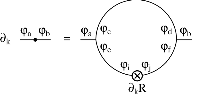
Figure 1: Diagrammatic form of the ERGEs for the parameters corresponding to terms quadratic in the fields in $\Gamma_{k}$. The external fields $\varphi_{a}$, $\varphi_{b}$ have to be chosen to be $A$, $H$, $c$, or $\bar{c}$ as described in the text. The crossed circle denotes an insertion of the function $\partial_{k}R^{k}(p^{2})$.

With $\bar{g}$ determined by (3.1) we have thus obtained a closed system of ERGEs for the 6 parameters $Z$, $n$, $m^{2}$, $h$, $\beta$ and $Z_{g}$. This is the minimal set which allows a) to parametrize the bare action (or the bare Lagrangian), and to obtain the correct 1-loop $\beta$ functions, and b) to parametrize a “confining” action where the parameters satisfy eq. (2.20). Since actually the quartic vertex without derivatives in $(F_{\mu\nu}^{a})^{2}$ does not contribute to the ERGEs in this approximation, all 6 ERGEs are of the same diagrammatic form as shown in fig. 1.

The type of external fields $\{\varphi_{a},\varphi_{b}\}$ and the powers of derivatives $\partial_{\mu}$ acting on them depend on the parameter, whose ERGE one is considering:

– $\{\varphi_{a},\varphi_{b}\}=\{A,A\}$ and ${\cal O}\left(\partial^{2}_{\mu}\right)$ in the case of $Z$,

– $\{\varphi_{a},\varphi_{b}\}=\{A,H\}$ and ${\cal O}\left(\partial_{\mu}\right)$ in the case of $n$,

– $\{\varphi_{a},\varphi_{b}\}=\{H,H\}$ and ${\cal O}\left(\partial_{\mu}^{0}\right)$ in the case of $m^{2}$,

– $\{\varphi_{a},\varphi_{b}\}=\{H,H\}$ and ${\cal O}\left(\partial^{2}_{\mu}\right)$ in the cases of $h$ and $\beta$,

– $\{\varphi_{a},\varphi_{b}\}=\{\bar{c},c\}$ and ${\cal O}\left(\partial^{2}_{\mu}\right)$ in the case of $Z_{g}$.

Note that two different Lorentz index structures are possible in the case $\{H,H\}$ and ${\cal O}\left(\partial^{2}_{\mu}\right)$, which have to be distinguished in order to separate the contributions to $h$ and $\beta$. The internal fields $\{\varphi_{i},\varphi_{j}\}$ attached to the insertion of $\partial_{k}R$ in fig. 1 have necessarily to be of the type $\{A,A\}$ or $\{\bar{c},c\}$, because only for these fields infrared cutoff terms $\Delta S_{k}$ exist. We have to take into account, however, mixed propagators of the type $\{\varphi_{e},\varphi_{i}\}=\{H,A\}$ or $\{\varphi_{c},\varphi_{d}\}=\{H,A\}$ etc., which lead to many different contributions even if the external fields $\{\varphi_{i},\varphi_{j}\}$ are fixed.

In order to exhibit the resulting ERGEs we employ the following notations: $P_{A}$, $P_{AH}$ etc. denote the propagator functions shown in eqs. (2.19), with the infrared cutoffs

$$R^{k}(p^{2})={e^{-p^{2}/k^{2}}\over 1-e^{-p^{2}/k^{2}}}$$ (3.3)

due to $\Delta S_{k}$ and the form of the functions $R_{\mu\nu}^{k}(p^{2})$ and $R_{g}^{k}(p^{2})$ (cf. eq. (2)) restored. This is easily done by replacing $Z\to Z+R^{k}$ and $Z_{g}\to Z_{g}+R^{k}$ in eqs. (2.19). Actually the exhibited form of the equations is general and allows for different choices of the cutoff function (3.3). (Our choice guarantees that all integrals appearing on the r.h. sides of the ERGEs are ultraviolet finite; however, we were not able to perform these momentum integrations analytically.)

Because of the required development in powers of derivatives (or external momenta) the quantities $p^{2}{\partial P_{A}\over\partial p^{2}}$ etc. appear frequently, and we define for convenience

$$P^{\prime}\equiv p^{2}\ {\partial P\over\partial p^{2}}\quad,\qquad P^{\prime\prime}\equiv p^{4}\ {\partial^{2}P\over(\partial p^{2})^{2}}$$ (3.4)

in all cases $P_{A}$, $P_{AH}$ etc. Finally we define $\partial_{k}\equiv k^{2}\partial/\partial k^{2}$, and performed the combinatories of the gauge group indices in the case of a $SU(N)$ gauge group. The 6 ERGEs then become

$$\partial_{k}\ Z = {N\bar{g}^{2}\over 16\pi^{2}}\int_{0}^{\infty}dp^{2}\ p^{4}\ \partial_{k}\ R^{k}\Big{[}Z^{2}\left({31\over 6}P_{A}^{3}+3P_{A}^{2}P^{\prime}_{A}+P_{A}^{2}P^{\prime\prime}_{A}\right)$$ (3.5a)

$$-nZ\Big{(}{16\over 3}P_{A}^{2}\ P_{AH}+{8\over 3}P_{A}\ P_{AH}\ P^{\prime}_{A}+P_{A}\ P_{AH}\ P^{\prime\prime}_{A}$$

$$+{10\over 3}P_{A}^{2}\ P^{\prime}_{AH}+P_{A}^{2}\ P^{\prime\prime}_{AH}\Big{)}$$

$$+n^{2}\Big{(}P_{A}\ P_{AH}\left({3\over 2}P^{\prime}_{AH}+{1\over 2}P^{\prime\prime}_{AH}\right)\Big{)}$$

$$+P^{2}_{AH}\left({5\over 12}P_{A}+{7\over 12}P^{\prime}_{A}+{1\over 4}P^{\prime\prime}_{A}\right)$$

$$+P_{A}^{2}\left({9\over 4}P^{\prime}_{HH,1}+{13\over 12}P^{\prime\prime}_{HH,1}+{3\over 4}P_{HH,2}+{11\over 12}P^{\prime}_{HH,2}+{1\over 4}P^{\prime\prime}_{HH,2}\right)$$

$$+{1\over 6}Z_{g}^{2}\ P_{g}^{3}\Big{]}\quad,$$

$$\partial_{k}\ n={N\bar{g}^{2}\over 16\pi^{2}}\int_{0}^{\infty}dp^{2}\ p^{4}\ \partial_{k}\ R^{k}\ n\ P_{A}^{2}\left({5\over 2}Z\ P_{A}-{3\over 2}n\ P_{AH}\right)\quad,$$ (3.5b)

$$\partial_{k}\ m^{2}={N\bar{g}^{2}\over 16\pi^{2}}\int_{0}^{\infty}dp^{2}\ p^{4}\ \partial_{k}\ R^{k}\ n^{2}\ P_{A}^{3}\quad,$$ (3.5c)

$$\partial_{k}\ Z_{g}={N\bar{g}^{2}\over 16\pi^{2}}\int_{0}^{\infty}dp^{2}\ p^{4}\ \partial_{k}\ R^{k}\ Z_{g}^{2}\ P_{A}\ P_{g}{3\over 4}\left(P_{A}+P_{g}\right)\quad,$$ (3.5d)

$$\partial_{k}\ h = {N\bar{g}^{2}\over 16\pi^{2}}\int_{0}^{\infty}dp^{2}\ p^{2}\ \partial_{k}\ R^{k}\ n^{2}\ P_{A}^{2}\left({1\over 6}P_{A}+{4\over 3}P^{\prime}_{A}+{2\over 3}P^{\prime\prime}_{A}\right)\quad,$$

$$\partial_{k}\beta = {1\over 2}\partial_{k}h\quad.$$ (3.5e)

Note that all integrals are trivially UV finite since, with the present choice of $R^{k}$, $\partial_{k}R^{k}$ decreases exponentially for large $p^{2}$, and IR finiteness is ensured by the presence of the IR cutoff terms in the propagators.

Let us first insert the “starting point values” (2.1) for the parameters on the r.h. sides of the ERGEs (3.5). Then all integrals can be performed analytically, and we should obtain the correct 1-loop $\beta$ functions. We find

$$\partial_{k}\ Z={Ng_{0}^{2}\over 16\pi^{2}}\cdot{31\over 6}\quad,$$

$$\partial_{k}\ n={Ng_{0}^{2}\over 16\pi^{2}}\cdot{7\over 4}\Lambda\quad,$$

$$\partial_{k}\ m^{2}={Ng_{0}^{2}\over 16\pi^{2}}\cdot{1\over 2}\Lambda^{2}\quad,$$

$$\partial_{k}\ h=-{Ng_{0}^{2}\over 16\pi^{2}}\cdot{7\over 12}\quad,$$

$$\partial_{k}\ Z_{g}={Ng_{0}^{2}\over 16\pi^{2}}\cdot{3\over 4}\quad.$$ (3.6)

This leads, indeed, to

$$\partial_{k}\ Z_{eff}=\partial_{k}\left(Z-{n^{2}\over m^{2}}\right)={Ng_{0}^{2}\over 16\pi^{2}}\cdot{13\over 6}\quad,$$ (3.7)

thus we obtain the correct 1-loop $\beta$ function for $g_{phys}$ as defined in eq. (3.2). From eqs. (3) and (3.7) one concludes that $Z$, $n$, $m^{2}$, $Z_{g}$ and $Z_{eff}$ start to decrease with decreasing $k^{2}$, whereas $h$ (and hence $\beta$, cf. (3)) start to increase.

The complete system of ERGEs (3.5) can be integrated numerically, with the choice of $g_{0}\equiv g_{phys}(\Lambda^{2})$ as the only freedom at the starting point. In fig. 2 we show a typical result obtained with $g_{0}=1.3$. We plot directly $Z_{eff}(k^{2})=Z(k^{2})-n^{2}(k^{2})/m^{2}(k^{2})$ and, for convenience, $\alpha_{phys}(k^{2})=g_{0}^{2}/(4\pi Z_{g}^{2}(k^{2})Z_{eff}(k^{2}))$ versus $-\ell n(k^{2}/\Lambda^{2})$. We find that at a small, but finite value of $k^{2}=k_{c}^{2}$ ($=1,94\cdot 10^{-5}\Lambda^{2}$ in the present case) both $Z_{g}(k_{c}^{2})$ and $Z_{eff}(k_{c}^{2})$ vanish, thus $\alpha_{phys}(k^{2})$ runs into a Landau singularity and the r.h. sides of the ERGEs (3.5) explode. The parameters $Z(k^{2})$, $n(k^{2})$ and $m^{2}(k^{2})$, however, remain finite and non-vanishing for $k^{2}\to k_{c}^{2}$ (in the present case we have $Z(k_{c}^{2})\cong 0.24$, $n(k_{c}^{2})\cong.43\cdot\Lambda$, $m^{2}(k_{c}^{2})\cong 0,76\cdot\Lambda^{2}$).

From the previous section, in particular from eq. (2.20) and the subsequent discussion, we know that a vanishing of $Z_{eff}(k_{c}^{2})$ corresponds to a confining form of the gluon propagator. In the corresponding expression eq. (2.21) a dimensionful quantity $\Lambda_{c}^{2}=m^{2}/\beta$ appears which could be related to the slope of a linearly rising $q\bar{q}$-potential obtained by a “dressed” one-gluon exchange (with a gluon propagator as in eq. (2.21)) in the non-relativistic limit. As such it should be independent from the starting scale $\Lambda$. However, $\Lambda$ is the only dimensionful scale in our approach, hence all dimensionful quantities are necessarily proportional to $\Lambda$. The physical meaning of $\Lambda$ is implicit in the choice of the bare coupling $g_{0}$: $g_{0}=g_{phys}(\Lambda^{2})$. Given the $\Lambda$-loop $\beta$ function for $g_{phys}$ (the 2-loop $\beta$ function is not obtained correctly within our approximation), the combined dependence of $\Lambda_{c}^{2}$ on $\Lambda^{2}$ and $g_{0}^{2}$ should thus be of the form

$$\Lambda_{c}^{2}=\Lambda^{2}\ e^{-(16\pi^{2}/11g_{0}^{2})}\left(1+{\cal O}\left({g_{0}^{2}\over 4\pi}\right)\right)\quad.$$ (3.8)

We have calculated the quantity

$$C={\Lambda^{2}\over\Lambda_{c}^{2}(k_{c}^{2})}\ e^{-(16\pi^{2}/11g_{0}^{2})}={\Lambda^{2}\beta(k_{c}^{2})\over m^{2}(k_{c}^{2})}\ e^{-(16\pi^{2}/11g_{0}^{2})}$$ (3.9)

for various choices of $g_{0}$, where the pattern of ERGE flow for all parameters is always of the form presented in the case $g_{0}=1.3$ (but with different results for $k_{c}^{2}/\Lambda^{2}$, of course): $g_{0}=1.3$: $C=1.68\cdot 10^{-2}$; $g_{0}=1.4$: $C=1.38\cdot 10^{-2}$; $g_{0}=1.5$: $C=1.20\cdot 10^{-2}$; $g_{0}=1.6$: $C=1,09\cdot 10^{-2}$; $g_{0}=1.7$: $C=1.01\cdot 10^{-2}$. Thus, although the corresponding values of $\Lambda_{c}^{2}(k_{c}^{2})/\Lambda^{2}$ vary over 2 orders of magnitude, $C$ remains approximately constant with an accuracy in agreement with eq. (3.8). (For even larger values of $g_{0}$ the ratio $\Lambda_{c}^{2}/\Lambda^{2}$ becomes larger than 1, i.e. the UV cutoff $\Lambda$ is below the “confinement scale” $\Lambda_{c}$, whereas for smaller values of $g_{0}$ the number of discrete steps for the integration of the ERGEs ($\sim\Lambda^{2}/k_{c}^{2}$) becomes extremely large without any new insight being gained).

Actually the fact that the “confining” relation $Z_{eff}(k_{c}^{2})=0$ and hence a Landau singularity in $\alpha_{phys}(k_{c}^{2})$ appears already at a finite value of $k^{2}=k_{c}^{2}$ is to be considered as an artefact of the present approximation to the ERGEs, which does evidently not yet capture the entire infrared dynamics of Yang-Mills theories (as, e.g., a possible gluon condensate). Focusing on the three parameters $Z$, $n$ and $m^{2}$, which appear in the “confining” relation (2.20), it is very interesting, however, that an analytic result can be obtained, which is independent of the other parameters: let us consider the r.h. sides of the corresponding ERGEs in the case where the relation $Z(k^{2})-n^{2}(k^{2})/m^{2}(k^{2})=0$ is fulfilled. In addition we assume that the scale $k^{2}$ is already far below the “confinement scale” $\Lambda_{c}^{2}=m^{2}/\beta$, $k^{2}\ll\Lambda_{c}^{2}$. Since only momenta with $p^{2}\raise 1.29167pt\hbox{$<$\kern-7.5pt\raise-4.73611pt\hbox{$\sim$}}k^{2}$ contribute to the integrals of the ERGEs (3.5) (remember the exponential damping), this assumption allows to simplify the propagators considerably and to obtain analytic results. We find

$$\partial_{k}\ Z={N\bar{g}^{2}\over 16\pi^{2}}\cdot{\Lambda_{c}^{2}\over k^{2}}\cdot{Z\over 4}\quad,$$

$$\partial_{k}\ n={N\bar{g}^{2}\over 16\pi^{2}}\cdot{\Lambda_{c}^{2}\over k^{2}}\cdot{n\over 4}\quad,$$

$$\partial_{k}\ m^{2}={N\bar{g}^{2}\over 16\pi^{2}}\cdot{\Lambda_{c}^{2}\over k^{2}}\cdot{m^{2}\over 4}\quad.$$ (3.10)

One easily derives

$$\partial_{k}\ Z_{eff}=\partial_{k}\left(Z-{n^{2}\over m^{2}}\right)={N\bar{g}^{2}\over 16\pi^{2}}\cdot{\Lambda_{c}^{2}\over k^{2}}\cdot{Z_{eff}\over 4}\quad,$$ (3.11)

i.e. whereas the individual parameters $Z$, $n$, and $m^{2}$ continue to run in a way which depends on the running of $\bar{g}^{2}$, $Z_{eff}=0$ is a quasi-fixed point of the ERGEs. Moreover, in agreement with our numerical analysis, this quasi-fixed point is infrared attractive. Were it not for the singular behaviour of $\bar{g}^{2}$ for small $k^{2}$ due to the vanishing of $Z_{g}$, the integrated eq. (3.11) would lead to a smooth vanishing of $Z_{eff}$ for $k^{2}\to 0$. Again, however, we cannot check in how far the quasi-fixed point $Z_{eff}=0$ depends on the present approximations to the ERGEs.

4 Conclusions

The intentions of the present paper are twofold: first, we proposed an effective low energy action for Yang-Mills theories, which involves an additional antisymmetric tensor field $H_{\mu\nu}^{a}$ introduced as an auxiliary field for the composite local operator $F_{\mu\nu}^{a}$. We have seen that, for a particular relation between 3 of the 6 parameters in this action, a confining gluon propagator in the sense of a $1/p^{4}$ behaviour for $p^{2}\to 0$ is obtained. On the other hand, we were able to relate this behaviour to a condensate of monopoles: the presence of the field $H_{\mu\nu}^{a}$ in the original action generates automatically the presence of a Goldstone boson $\varphi$ in the dual action (of the abelian subsystem), which is thus of the form of an abelian Higgs model in the broken phase (with frozen radial excitations). This “dual” role of the auxiliary field $H_{\mu\nu}^{a}$ is certainly a particular feature of gauge theories in $d=4$ dimensions. An amazing and conceptually important feature is the fact that, from the point of view of the original action, the confining behaviour of the gluon propagator is not directly related to a non-trivial vacuum (it can be speculated, however, that a vanishing of $Z_{eff}$ is a necessary condition for the formation of a gluon condensate).

Second, we have discussed a dynamical scheme, which allows to compute the corresponding low energy effective action from the bare Yang-Mills Lagrangian: the Wilsonian ERGEs including auxiliary fields. Since this constitutes, a priori, an exact formalism, it allows for various approximations in order to turn it into a closed system of differential equations. These approximations can be chosen such that they correspond to the physical problem under consideration. Here we did not solve the ERGEs for the parameters corresponding to higher dimensional or non-BRST-invariant terms in the effective action, whose knowledge is not required for the check of the “confining relation” eq. (2.20). The approximation consisted then in the neglect of the contributions of these parameters to the ERGEs of the 6 important parameters $Z$, $n$, $m^{2}$, $h$, $\beta$ and $Z_{g}$. We have seen that, within this approximation, the relation (2.20) constitutes indeed an infrared attractive quasi-fixed point of the ERGEs. On the other hand, the fact that the relation (2.20) is assumed already at a finite scale $k^{2}=k_{c}^{2}$, and the physical gauge coupling runs into a Landau singularity, is obviously an artifact of the approximation. We have certainly not yet solved the problem of finding approximations to the system of ERGEs, which allow to obtain numerically reliable results in the infrared.

However, the present approach may point into a direction where this problem may be solvable. We have seen that the duality transformation of the abelian subsystem provides us with the action of an abelian Higgs model in the broken phase. This model has trivial infrared fixed points in the Wilsonian sense, since it contains no massless physical fields which could contribute to the ERGE flow in the limit $k^{2}\sim p^{2}\to 0$. Duality transformations can also be considered for full non-abelian actions, see [26] for first steps in this direction. Here the genuine problem is that one obtains actions, which are non-local, non-polynomial in the fields, and/or involve additional auxiliary degrees of freedom. On the other hand, all these features are already present in Wilsonian effective actions in general, and the Wilsonian functional ERGE is capable to cope with then. Let us now speculate that the result of a duality transformation of a full non-abelian action, again in the presence of auxiliary fields $H_{\mu\nu}^{a}$, leads us again to dual actions which contain no massless physical fields. Then we would obtain automatically infrared fixed points for the Wilsonian ERGEs for the dual action, which allow to obtain numerically reliable results in the infrared. It then remains to reinterpret the infrared effective action of the dual theory in terms of the original theory in order to extract its physical consequences. Although we are aware of the speculative nature of this approach it is presently under investigation.

Figure 2: Result of the numerical integration of the ERGEs (3.5) with $g_{0}=1.3$. $Z_{eff}(k^{2})$ and $\alpha_{phys}(k^{2})$ are defined in eq. (2.17) and below eq. (3.7), respectively. The ERGE flow starts at $-\ell n(k^{2}/\Lambda^{2})=0$ and stops due to the Landau singularity at $-\ell n(k^{2}_{c}/\Lambda^{2})\sim 10.85$.

References

- [1]
- [2] S. Mandelstam, Phys. Rep. 23C (1976) 245; G. t’Hooft, Nucl. Phys. B190 (1981) 455.
- [3] Lattice 96, Proceedings; Nucl. Phys. B (Proc. Suppl.) 53 (1997).
-
[4]
A. Polyakov, JETP Lett. 20 (1974) 194;
G. t’Hooft, Nucl. Phys. B79 (1974) 276. - [5] M. Blagojevic, P. Senjanovic, Phys. Rep. 157 (1988) 233.
- [6] A. Di Giacomo, M. Mathur, Phys. Lett. B400 (1997) 129.
-
[7]
K. Bardakci, S. Samuel, Phys. Rev. D18 (1978)
2849;
E. Akhmedov, M. Chernodub, M. Polikarpov, M. Zubkov, Phys. Rev. D53 (1996) 2087. - [8] D. Zwanziger, Phys. Rev. D3 (1971) 880.
- [9] M. Mathur, H. Sharatchandra, Phys. Rev. Lett. 66 (1991) 3097.
- [10] K. Lee, Phys. Rev. D48 (1993) 2493.
- [11] S. Maedan, Y. Matsubara, T. Suzuki, Prog. Theor. Phys. 84 (1990) 130 and refs. therein.
-
[12]
M. Baker, J. Ball, F. Zachariasen, Phys. Rep. 209
(1991) 73, Int. J. Mod. Phys.
A11 (1996) 343;
M. Baker, J. Ball, N. Brambilla, G. Prosperi, F. Zachariasen, Phys. Rev. D54 (1996) 2829. -
[13]
K. Wilson and I. Kogut, Phys. Rep. 12 (1974) 75;
F. Wegner, in: Phase Transitions and Critical Phenomena, Vol. 6, eds. C. Domb and M. Green (Academic Press, NY 1975). -
[14]
S. Weinberg, in: Proceedings of the 1976 International
School of Subnuclear Physics,
Erice, ed. A. Zichichi;
J. Polchinski, Nucl. Phys. B231 (1984) 269. -
[15]
G. Keller, C. Kopper, Phys. Lett. B273
(1991) 323;
G. Keller, C. Kopper, M. Salmhofer, Helv. Phys. Acta 65 (1997) 32;
C. Wetterich, Phys. Lett. B301 (1993) 90;
C. Wetterich, M. Reuter, Phys. Lett. B334 (1994) 412;
T. Morris, Int. J. Mod. Phys. A9 (1994) 2411;
M. D’Attanasio, T. Morris, Phys. Lett. B378 (1996) 213;
For more references see J. Comellas, Y. Kubyshin, E. Moreno, Nucl. Phys. B490 (1997) 653. -
[16]
C. Becchi, in: Lectures given at the Summer School
in Theoretical Physics, Parma
1991-1993, eds. M. Bonini, G. Marchesini and E. Onofri,
Parma University 1993;
M. Bonini, M. D’Attanasio, G. Marchesini, Nucl. Phys. B418 (1994) 81, Nucl. Phys. B421 (1994) 429, Nucl. Phys. B437 (1995) 163, Phys. Lett. B346 (1995) 87. - [17] U. Ellwanger, Phys. Lett. B335 (1994) 364.
- [18] U. Ellwanger, Z. Phys. C58 (1993) 619.
- [19] U. Ellwanger, C. Wetterich, Nucl. Phys. B423 (1994) 137.
-
[20]
U. Ellwanger, M. Hirsch, A. Weber, Z. Phys. C69
(1996) 687 and hep-ph/9606468,
to appear in Z. Phys. C;
U. Ellwanger, hep-ph/9702309, to appear in Z. Phys. C;
B. Bergerhoff, C. Wetterich, hep-ph/9708425. - [21] R. Haymaker, Riv. Nuovo Cim. 14 (1991), No. 8.
-
[22]
M. Holperu, Phys. Rev. D16 (1977) 1798;
M. Quandt, H. Reinhardt, hep-th/9707185 and refs. therein. - [23] G. West, Phys. Lett. B115 (1982) 468.
- [24] C. Roberts and A. Williams, Prog. in Part. and Nucl. Physics 33 (1994) 477, and references therein.
- [25] K. Kondo, preprint CHIBA-EP-99, hep-th/9709109.
-
[26]
K. Itabashi, Prog. Theor. Phys. 65 (1981) 1423;
L. Mizrachi, Annals Phys. 153 (1984) 417 and Phys. Lett. B139 (1984) 374;
A. Caticha, Phys. Rev. D37 (1988) 2323.