Abstract

Cut vertices, a generalization of matrix elements of local operators, are revisited, and an expansion in terms of minimally subtracted cut vertices is formulated. An extension of the formalism to deal with semi-inclusive deep inelastic processes in the target fragmentation region is explicitly constructed. The problem of factorization is discussed in detail.

1 Introduction

Factorization theorems [1, 2] are an essential tool in QCD hard processes since they allow to separate short-distance from long-distance effects. The former, due to asymptotic freedom, are calculable in perturbation theory, while the latter can be parameterized into phenomenological distributions.

Factorization theorems are proved by showing that cross sections develop collinear singularities occurring in a universal factorized fashion, while soft singularities, which could in principle spoil such a picture, cancel out.

Operator Product Expansion (OPE) [3, 4] as well is a powerful method to separate short-distance from long-distance effects but it has unfortunately found practical applications only in the context of inclusive Deep Inelastic Scattering (DIS). This stems from the fact that OPE works for amplitudes in particular kinematic regions whereas to describe physical processes one needs a prediction for cross sections, i.e. cut amplitudes. However there is a generalization of OPE, the cut vertex expansion, originally proposed by Mueller [5], that allows to treat processes different from DIS, since it directly deals with cross sections. With this method the cross section for DIS ($e^{+}e^{-}\to h+X$) factorizes into a spacelike (timelike) cut vertex convoluted with a coefficient function. The former contains the long-distance behavior while the latter is calculable as usual in perturbation theory. In the context of DIS this expansion is equivalent to the one obtained by applying OPE, as it can be proved that a spacelike cut vertex is actually equivalent to a matrix element of a minimal twist local operator [6, 7]. Nevertheless the cut vertex expansion holds also in $e^{+}e^{-}\to h+X$ and in this case the cut vertex corresponds to a non-local operator. In Ref.[6] a parton model interpretation of cut vertices was given. In such a picture a spacelike cut vertex is in some sense equivalent to a parton distribution, whereas a timelike cut vertex corresponds to a fragmentation function. The cut vertex technique has been applied in Ref.[8] to a variety of hard processes.

We remarked that a cut vertex is a (generally non-local) operator and therefore it needs renormalization. Cut vertex renormalization was originally proposed in the collinear subtraction scheme [5] but one can work in the MS scheme with minor modifications [9] and here the coefficient function is expected to be analytical in the zero mass limit [10].

Let us now consider the semi-inclusive process $p+J(q)\to p^{\prime}+X$. In the region in which the transverse momentum of the observed hadron, or equivalently the momentum transfer $t=-(p-p^{\prime})^{2}$, is of order of the hard scale $Q^{2}$, the cross section can be written either as a convolution of a parton density with a hard cross section and a fragmentation function, or, in the language of cut vertices, as a convolution of a spacelike with a timelike cut vertex through a coefficient function. However a similar picture does not work in the limit $t\ll Q^{2}$ since in that region the cross section is dominated by the target fragmentation mechanism.

In a recent paper [11] an extension of the cut vertex approach has been proposed in order to deal with semi-inclusive DIS in the target fragmentation region. It has been argued that a generalized cut vertex expansion holds in the limit $t\ll Q^{2}$. This fact has relevant phenomenological consequences. As shown in Ref.[11], once such an expansion is proved, it is possible to define a new object, an extended fracture function ${\cal M}_{A,A^{\prime}}^{i}(x,z,t,Q^{2})$, just in terms of a new cut vertex. Whereas ordinary fracture functions [12] give the probability of extracting a parton $i$ with momentum fraction $x$ from an incoming hadron $A$, observing another hadron $A^{\prime}$ with momentum fraction $z$ in the final state, extended fracture functions depend on the further scale $t$ at which $A^{\prime}$ is detected.

In the present paper we want to construct explicitly such a generalized cut vertex expansion and we will eventually show that this program can be carried out with no substantial complication. The model we will work in is $(\phi^{3})_{6}$, which, despite its simpler structure, shares several important aspects with QCD: it is asymptotically free and the topology of the leading diagrams resembles that of QCD in a physical gauge. The cut vertex method, which, as a generalization of OPE, is based on Zimmermann formalism [4], combined with infrared power counting techniques [2, 13], will allow us to formulate an expansion of the semi-inclusive cross section in the target fragmentation region into a new MS cut vertex convoluted with the same coefficient function appearing in inclusive DIS.

The paper is organized as follows. In Sect. 2 we will review the cut vertex formalism, first with some examples and then showing how an expansion in terms of minimally subtracted cut vertices can be given. In Sect. 3 we will generalize the cut vertex formalism to semi-inclusive DIS. In Sect. 4 we will discuss factorization and in Sect. 5 we will sketch our conclusions.

2 A cut vertex expansion

2.1 Examples

Cut vertices arise quite naturally when dealing with processes characterized by a large momentum transfer. Let us consider DIS in $\phi^{3}_{6}$

$$p+J(q)\rightarrow X$$

with the current $J=\frac{1}{2}\phi^{2}$. The structure function is defined as

$$F(p,q)=\frac{Q^{2}}{2\pi}\int e^{iqx}<p|J(x)J(0)|p>.$$ (2.1.1)

We choose a frame in which $p=(p_{+},{\bf 0},p_{-})$, with $p_{+}\gg p_{-}$ and $pq\simeq p_{+}q_{-}$. Given a vector $k=(k_{+},{\bf k},k_{-})$ define ${\hat{k}}=(k_{+},{\bf 0},0)$. We now consider the ladder contribution to the structure function, represented in Fig.1.

Figure 1: A one loop contribution to DIS in $(\phi^{3})_{6}$

We have

$$W_{1}(p,q)=\int V_{1}(p,k)M_{1}(k,q)\frac{d^{6}k}{(2\pi)^{6}}$$ (2.1.2)

where

$$V_{1}(p,k)=2\pi\lambda^{2}\delta_{+}((p-k)^{2})\frac{1}{k^{4}}$$ (2.1.3)

$$M_{1}(k,q)=Q^{2}\delta_{+}((k+q)^{2}).$$ (2.1.4)

In the limit $p^{2}\to 0$ this graph develops a collinear singularity which corresponds to the configuration in which $k$ is parallel to $p$. Hence in the integration in (2.1.2) two distinct regions give contribution in the large $Q^{2}$ limit

$$(a)~{}~{}~{}\mbox{collinear:}~{}~{}~{}k^{2}\ll Q^{2}\mbox{ and }k\parallel p$$

$$(b)~{}~{}~{}\mbox{UV:}~{}~{}~{}~{}~{}~{}~{}~{}~{}~{}k^{2}\sim Q^{2}.$$ (2.1.5)

Factorization is proved by arranging the integral (2.1.2) so as to isolate the contributions in these regions:

$$W_{1}(p,q) =\int V_{1}(p,k)M_{1}(\hat{k},q)\frac{d^{6}k}{(2\pi)^{6}}+\int V_{1}(\hat{p},k)\left(M_{1}(k,q)-M_{1}(\hat{k},q)\right)\frac{d^{6}k}{(2\pi)^{6}}$$

$$+\int\Big{(}V_{1}(p,k)-V_{1}(\hat{p},k)\Big{)}\Big{(}M_{1}(k,q)-M_{1}(\hat{k},q)\Big{)}\frac{d^{6}k}{(2\pi)^{6}}.$$ (2.1.6)

The first term dominates in the collinear region, while the second is important in the UV region. The third term is the remainder and is manifestly suppressed by a power of $1/Q^{2}$. The operation we performed is called oversubtraction: it is a subtraction in addition to standard UV renormalization and aims at isolating the leading part of the cross section.

It is now straightforward to show that the first two terms in (2.1) can be written in a factorized form. If we define the bare cut vertex $v^{(0)}(p^{2},x)=\delta(1-x)$ and its one loop radiative correction (see Fig.2)

Figure 2: (a) The bare cut vertex (b) One of its radiative corrections

$$v^{(1)}(p^{2},x)=\int V_{1}(p,k)x\delta\left(x-\frac{k_{+}}{p_{+}}\right)\frac{d^{6}k}{(2\pi)^{6}}$$ (2.1.7)

we can write

$$W_{1}(p,q) \simeq\int\frac{du}{u}v^{(1)}(p^{2},u)C^{(0)}(x/u,Q^{2})+\int\frac{du}{u}v^{(0)}(p^{2},u)C^{(1)}_{1}(x/u,Q^{2})$$

$$=\int\frac{du}{u}v(p^{2},u)C_{1}(x/u,Q^{2})\Big{|}_{order\lambda^{2}}$$ (2.1.8)

where

$$C^{(0)}(x,Q^{2})=M_{1}(0,x,Q^{2})$$ (2.1.9)

$$C^{(1)}_{1}(x,Q^{2})=\int V_{1}(\hat{p},k)\left(M_{1}(k,q)-M_{1}(\hat{k},q)\right)\frac{d^{6}k}{(2\pi)^{6}}$$ (2.1.10)

and it appears that factorization works as in Fig.3.

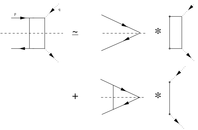
Figure 3: Factorization of the ladder diagram in $(\phi^{3})_{6}$

As usual a simpler factorized expression can be obtained by taking moments with respect to $x$. Defining the Mellin transform as

$$f_{\sigma}=\int^{1}_{0}dxx^{\sigma-1}f(x)$$ (2.1.11)

we get

$$W_{1}^{\sigma}(p^{2},Q^{2})=v_{\sigma}(p^{2})C_{1}^{\sigma}(Q^{2}).$$ (2.1.12)

Actually both the terms in (2.1) are UV divergent expressions. Nevertheless, due to the finiteness of the initial integral, divergences can be removed by adding and subtracting a suitable UV counterterm, as we will clarify in the next section.

Figure 4: A virtual correction to the DIS in $(\phi^{3})_{6}$

Let us now consider the graph in Fig.4. In the large $Q^{2}$ limit it gives

$$W_{2}(p,q)=-\frac{1}{2}\delta(1-x)\frac{\lambda^{2}}{(4\pi)^{3}}\left(\log\frac{Q^{2}}{4\pi\mu^{2}}+\mbox{finite terms}\right)$$ (2.1.13)

where the proper MS counterterm has been added in order to cure the ordinary UV divergence. Whereas in the previous example there was a divergence in the limit $p^{2}\to 0$, which is a signal of long-distance dependence, here the limit $p^{2}\to 0$ is harmless. Hence

$$W_{2}(p,q)=\int v^{(0)}(p^{2},u)C^{(1)}_{2}(x/u,Q^{2})$$ (2.1.14)

with

$$C^{(1)}_{2}(x,Q^{2})=W_{2}(0,x,Q^{2})$$ (2.1.15)

that is factorization works as in Fig.5. Thus the unique leading contribution is obtained when a large momentum flows in the loop, and no long-distance contribution arises from this graph which gives only a correction to the coefficient function.

Figure 5: Its decomposition in the large $Q^{2}$ limit

In the following we will generalize this construction for a general graph: the leading contributions to the DIS structure function in $(\phi^{3})_{6}$ are given by the decomposition depicted in Fig.6.

Figure 6: Relevant decomposition for DIS in $(\phi^{3})_{6}$

Here $\tau$ is the hard subgraph, that is the part of the graph in which a large momentum flows, and $\lambda$ is the soft subgraph. Decompositions with more than two legs connecting the hard to the soft subgraph are suppressed by powers of $1/Q^{2}$. By using this fact and Zimmermann formalism [4] we will be able to define a cut vertex expansion at all orders.

2.2 Cut vertex expansion for DIS in $(\phi^{3})_{6}$

Let us consider a general graph $\Gamma$ giving contribution to the deep inelastic structure function, renormalized for example in the MS scheme. We saw that the strategy which allows to isolate the leading term in the structure function consists in oversubtractions. In order to implement this program at all orders we need a definition of renormalization part and of a subtraction operator. First of all we define the graph ${\tilde{\Gamma}}$ as $\Gamma$ in which the vertices of insertion of $J$ are merged at the same point $V$ (see Fig.7).

Figure 7: (a) general cut graph $\Gamma$ contributing to the DIS structure function (b) the graph obtained from $\Gamma$ by merging the currents at the same point $V$

Keeping in mind the conclusions of the previous subsection we define a renormalization part $\gamma$ as a subgraph of $\Gamma$ such that ${\tilde{\gamma}}$ is either the bare cut vertex or a proper subdiagram of ${\tilde{\Gamma}}$ containing $V$ with two external legs. As usual a forest $\cal U$ of $\Gamma$ is a set of non overlapping renormalization parts of $\Gamma$. A forest may be empty.

Given a renormalization part $\gamma$ of $\Gamma$, its contribution in the loop integral as a function of external momenta must be of the form $I_{\gamma}(k,q)$. We define the subtraction operator $t^{\gamma}$ as

$$t^{\gamma}I_{\gamma}(k,q)=I_{\gamma}(\hat{k},q).$$ (2.2.1)

Now, as we have done in the previous examples, we have to relate the structure function, the leading term and the remainder through an identity.

Given the graph $\Gamma$ the contribution to the structure function is

$$W_{\Gamma}(p,q)=\int J_{\Gamma}(p,k_{1}...k_{l},q)\frac{d^{6}k_{1}}{(2\pi)^{6}}...\frac{d^{6}k_{l}}{(2\pi)^{6}}\equiv I_{\Gamma}$$ (2.2.2)

where $k_{i},i=1...l$ is the set of loop momenta to be integrated over. We define

$$X_{\Gamma}=\sum_{\cal U(\Gamma)\neq\emptyset}~{}\prod_{\gamma\in\cal U}\left(-t^{\gamma}\right)I_{\Gamma}$$ (2.2.3)

$$Z_{\Gamma}=\sum_{{\cal U}_{t}(\Gamma)}~{}\prod_{\gamma\in{\cal U}_{t}}\left(-t^{\gamma}\right)I_{\Gamma}$$ (2.2.4)

$$Y_{\Gamma}=-\sum_{{\cal U}_{t}(\Gamma)}~{}\prod_{\gamma\in{\cal U}_{t}}\left(-t^{\gamma}\right)\left(-t^{\gamma_{t}}\right)I_{\Gamma}$$ (2.2.5)

where ${\cal U}_{t}(\Gamma)$ are $\Gamma$ forests which do not contain the bare cut vertex as renormalization part, and $\gamma_{t}$ is the bare cut vertex. The following identity holds [4, 10]

$$W_{\Gamma}=-X_{\Gamma}+Z_{\Gamma}-Y_{\Gamma}.$$ (2.2.6)

The claim is that in (2.2.6) $-X_{\Gamma}$ is the leading term while $Z_{\Gamma}-Y_{\Gamma}$ is the remainder and is suppressed in the large $Q$ limit.

The next step is to show that $X_{\Gamma}$ has a factorized structure. The definition of renormalization part we have given is such that the renormalization parts in a forest $\cal U$ are all nested. Therefore it is possible to select the innermost renormalization part $\gamma_{0}$ and the expression for $X_{\Gamma}$ can be recast in the form

$$X_{\Gamma}=-\sum_{\gamma_{0}}\sum_{{\cal U}_{t}(\Gamma/\gamma_{0})}~{}\prod_{\gamma\in{\cal U}_{t}(\Gamma/\gamma_{0})}(-t^{\gamma})\int\frac{d^{6}k}{(2\pi)^{6}}I_{\Gamma/\gamma_{0}}(p,k)~{}t^{\gamma_{0}}I_{\gamma_{0}}(k,q),$$ (2.2.7)

where we used our definition of renormalization part. By taking moments we get a completely factorized expression

$$\left(W_{\Gamma}\right)_{\sigma}\sim-\left(X_{\Gamma}\right)_{\sigma} =\sum_{\gamma_{0}}\sum_{{\cal U}_{t}(\Gamma/\gamma_{0})}~{}\prod_{\gamma\in{\cal U}_{t}(\Gamma/\gamma_{0})}(-t^{\gamma})\tilde{v}_{\Gamma/\gamma_{0}}^{\sigma}(p^{2})~{}\tilde{C}^{\sigma}_{\gamma_{0}}(Q^{2})$$

$$=\sum_{\gamma_{0}}\bar{v}_{\Gamma/\gamma_{0}}^{\sigma}(p^{2})\bar{C}^{\sigma}_{\gamma_{0}}(Q^{2})\equiv v_{\sigma}^{M}(p^{2})C^{M}_{\sigma}(Q^{2})$$ (2.2.8)

where

$$\tilde{v}_{\Gamma/\gamma_{0}}^{\sigma}(p^{2}) =\int_{0}^{1}dxx^{\sigma-1}\int I_{\Gamma/\gamma_{0}}(p,k)x\delta\left(x-\frac{k_{+}}{p_{+}}\right)\frac{d^{6}k}{(2\pi)^{6}}$$

$$=\int I_{\Gamma/\gamma_{0}}(p,k)\left(\frac{k_{+}}{p_{+}}\right)^{\sigma}\theta(k_{+})\frac{d^{6}k}{(2\pi)^{6}}$$ (2.2.9)

and

$$\tilde{C}^{\sigma}_{\gamma_{0}}(Q^{2})=\int_{0}^{1}dxx^{\sigma-1}I_{\gamma_{0}}(0,x,Q^{2})$$ (2.2.10)

are the unrenormalized cut vertex and coefficient function respectively, while $\bar{v}_{\Gamma/\gamma_{0}}^{\sigma}(p^{2})$ and $\bar{C}^{\sigma}_{\gamma_{0}}(Q^{2})$ are renormalized quantities. We saw in the previous subsection that in the large $Q$ limit separately divergent contributions may arise even if we start from a UV finite integral. In eq. (2.2) the operator acting on $\tilde{v}_{\Gamma/\gamma_{0}}^{\sigma}(p^{2})$ performs cut vertex renormalization by using the same prescription adopted in oversubtraction. Thus eq. (2.2) is just the cut vertex expansion proposed by Mueller in Ref.[5], with the only difference that in Ref.[5] the ordinary UV renormalization was explicitly performed with zero momentum subtraction, whereas here we have worked with renormalized quantities.

In this paper we prefer to use minimally subtracted cut vertices [9], and so doing we slightly modify the expression for $X_{\Gamma}$ by following Ref.[10].

From now on we will work in $d=6-2\epsilon$ dimensions and define the operator $t^{\gamma}_{\epsilon}$ as acting on a renormalization part $\gamma$ by annihilating all terms which are not singular as $\epsilon\to 0$. A particular $t^{\gamma}_{\epsilon}$ acts after the loop integrals inside $\gamma$ are performed, and the ordinary UV counterterms added.

Given a forest $\cal U(\Gamma)\neq\emptyset$ call $\tau$ the outermost $\gamma\in\cal U(\Gamma)$ and let $\tilde{\cal U}(\tau)$ be a forest of $\Gamma$ such that $\gamma\in\tilde{\cal U}(\tau)\Leftrightarrow\gamma\supseteq\tau$. Furthermore, define $\tilde{\cal U}_{t}(\tau)$ a forest of $\Gamma$ such that $\gamma\in\tilde{\cal U}_{t}(\tau)\Leftrightarrow\gamma\supsetneq\tau$. The quantity

$$X_{\Gamma}^{\prime}=\sum_{\cal U(\Gamma)\neq\emptyset}~{}\sum_{\tilde{\cal U}(\tau)}~{}\prod_{\gamma\in\tilde{\cal U}}(-t^{\gamma}_{\epsilon})\prod_{\gamma\in\cal U}(-t^{\gamma})I_{\Gamma}$$ (2.2.11)

differs from $X_{\Gamma}$ in that it contains extra UV counterterms which make each forest contribution separately finite. However, $X_{\Gamma}$ is free from UV divergences, so that extra counterterms in $X_{\Gamma}^{\prime}$ must cancel and we have $X^{\prime}_{\Gamma}=X_{\Gamma}$. $X^{\prime}_{\Gamma}$ can be rearranged in the form

$$X_{\Gamma}^{\prime} =-\sum_{\tau}\sum_{\tilde{\cal U}_{t}(\tau)}\prod_{\gamma\in\tilde{\cal U}_{t}}(-t^{\gamma}_{\epsilon})(1-t_{\epsilon}^{\tau})t^{\tau}\sum_{{\cal U}^{n}(\tau)}\prod_{\gamma\in{\cal U}^{n}}(-t^{\gamma})I_{\Gamma}$$

$$=-\sum_{\tau}\int\frac{d^{D}k}{(2\pi)^{D}}\sum_{\tilde{\cal U}_{t}(\tau)}\prod_{\gamma\in\tilde{\cal U}_{t}}(-t^{\gamma}_{\epsilon})I_{\Gamma/\tau}(p,k)(1-t_{\epsilon}^{\tau})t^{\tau}\sum_{{\cal U}^{n}(\tau)}\prod_{\gamma\in{\cal U}^{n}}(-t^{\gamma})I_{\tau}(k,q)$$ (2.2.12)

where ${\cal U}^{n}(\tau)$ are the normal forests of $\tau$, i.e. forests of $\tau$ which do not contain $\tau$. Eq.(2.2) can be easily derived by observing that

$$\prod_{\gamma\in\cal U}(-t^{\gamma})I_{\Gamma}=(-t^{\tau})\prod_{\gamma\in{\cal U}^{n}(\tau)}(-t^{\gamma})I_{\Gamma}$$ (2.2.13)

and that the forest $\tilde{\cal U}(\tau)$ can either contain $\tau$ or not:

$$\sum_{\tilde{\cal U}(\tau)}~{}\prod_{\gamma\in\tilde{\cal U}}(-t^{\gamma}_{\epsilon})=\sum_{\tilde{\cal U}_{t}(\tau)}~{}\prod_{\gamma\in\tilde{\cal U}_{t}}(-t^{\gamma}_{\epsilon})(1-t_{\epsilon}^{\tau}).$$ (2.2.14)

Let us comment on the structure of eq. (2.2). Given a maximal renormalization part $\tau$, a decomposition as in Fig.6 follows. The operator acting on $I_{\tau}(k,q)$ performs subtractions corresponding to possible renormalization parts $\gamma$ contained into $\tau$. The operator $t^{\tau}$ replaces $k$ with ${\hat{k}}$ as in the examples of the previous subsection and $(1-t^{\tau}_{\epsilon})$ removes possible UV divergences, so that what we get on the right is the coefficient function. On the left the operator acting on $I_{\Gamma/\tau}(p,k)$ renormalizes the cut vertex, now in the MS scheme. Thus, by taking moments, we can write

$$\left(W_{\Gamma}\right)_{\sigma}\simeq-\left(X_{\Gamma}\right)_{\sigma} =\sum_{\tau}\sum_{\tilde{\cal U}_{t}(\tau)}\prod_{\gamma\in\tilde{\cal U}_{t}}(-t^{\gamma}_{\epsilon})\tilde{v}^{\sigma}_{\Gamma/\tau}(p^{2})(1-t_{\epsilon}^{\tau})\sum_{{\cal U}^{n}(\tau)}\prod_{\gamma\in{\cal U}^{n}}(-t^{\gamma})\tilde{C}_{\tau}^{\sigma}(Q^{2})$$

$$=\sum_{\tau}v^{\sigma}_{\Gamma/\tau}(p^{2})C^{\sigma}_{\tau}(Q^{2})\equiv v_{\sigma}(p^{2})C_{\sigma}(Q^{2})$$ (2.2.15)

that is to say, we end up with a completely factorized expression. Here $v^{\sigma}_{\Gamma/\tau}(p^{2})$ and $C^{\sigma}_{\tau}(Q^{2})$ are the renormalized cut vertex and coefficient function in the MS scheme respectively.

Finally we want to show how eq. (2.2) works with the examples considered before.

Figure 8: The diagram ${\tilde{\Gamma}}_{1}$ and its subdiagrams ${\tilde{\gamma}_{1}}$ and ${\tilde{\gamma}_{2}}$

Let us go back to the diagram in Fig.1 and call it $\Gamma_{1}$. The diagram ${\tilde{\Gamma}}_{1}$ is represented in Fig.8 and $\gamma_{1}$ and $\gamma_{2}$ appear to be the renormalization parts. From eq. (2.2) we obtain

$$W_{1}(p,q)\simeq-X_{\Gamma_{1}} =\int(1-t_{\epsilon}^{\gamma_{2}})I_{\Gamma_{1}/\gamma_{1}}(p,k)t^{\gamma_{1}}I_{\gamma_{1}}(k,q)\frac{d^{D}k}{(2\pi)^{D}}$$

$$+\int I_{\Gamma_{1}/\gamma_{2}}(p,k)(1-t_{\epsilon}^{\gamma_{2}})t^{\gamma_{2}}(1-t^{\gamma_{1}})I_{\gamma_{2}}(k,q)\frac{d^{D}k}{(2\pi)^{D}}$$ (2.2.16)

By taking moments we get the renormalized form of eq. (2.1) in the MS scheme.

Then consider the diagram in Fig.4 and call it $\Gamma_{2}$. The corresponding diagram ${\tilde{\Gamma}}_{2}$ is represented in Fig.9. The graph itself gives the only renormalization part $\gamma$ and so eq. (2.2) reads

$$W_{2}(p,q)\simeq\int I_{\Gamma_{2}/\gamma}(p,k)t^{\gamma}I_{\gamma}(k,q)\frac{d^{6}k}{(2\pi)^{6}}=W_{2}(0,x,Q^{2}).$$ (2.2.17)

Figure 9: The diagram ${\tilde{\Gamma}}_{2}$ shows that $\Gamma_{2}$ has only one renormalization part which is the graph itself

Eventually we should show that the expansion outlined in this section corresponds indeed to the leading contribution or, equivalently, the remainder is suppressed by a power of $1/Q^{2}$. Naively this happens since all the leading momentum flows are subtracted off [5], but we will provide a more precise argument in Sect. 4. Nevertheless it can be shown [6, 7] that the spacelike cut vertex represents the analytic continuation in the spin variable of the matrix element of minimal twist operator $O_{\mu_{1}...\mu_{n}}=\phi(0)\partial_{\mu_{1}}...\partial_{\mu_{n}}\phi(0)$. Thus the cut vertex expansion is equivalent in this case to OPE and we do not need to exhibit any additional proof.

3 Generalized cut vertex expansion

3.1 Examples

Here we are going to discuss the process $p+J(q)\to p^{\prime}+X$. In this case a semi-inclusive structure function can be defined

$$W(p,p^{\prime},q)=\frac{Q^{2}}{2\pi}\sum_{X}\int d^{6}xe^{iqx}<p|J(x)|p^{\prime}X><Xp^{\prime}|J(0)|p>$$ (3.1.1)

and let $z$ be

$$z=\frac{p^{\prime}q}{pq}.$$ (3.1.2)

In Ref.[11] it was argued that in the region $t\ll Q^{2}$ an expansion similar to (2.2) holds for the semi-inclusive structure function. In Ref.[14] a one loop calculation of the semi-inclusive cross section has been performed which confirms such expectation. We will now point out how to perform such a generalization, and, as we did before, we will start with some examples. Consider the diagram in Fig.10, which takes into account real emission from the initial leg.

Figure 10: A one loop contribution to the semi-inclusive structure function

We have

$$W_{1}(p,p^{\prime},q)=\int V_{1}(p,p^{\prime},k)M_{1}(k,q)\frac{d^{6}k}{(2\pi)^{6}}$$ (3.1.3)

where

$$V_{1}(p,p^{\prime},k)=\lambda^{4}2\pi\delta_{+}\left((p-k-p^{\prime})^{2}\right)\frac{1}{k^{4}}\frac{1}{(k+p^{\prime})^{4}}$$ (3.1.4)

and $M_{1}(k,q)$ is given by eq. (2.1.4). In the region $t\ll Q^{2}$ the integral gets its leading contribution in the region of small transverse momentum ${\bf k}_{\perp}$ [14], and so we can write

$$W_{1}(p,p^{\prime},q)\simeq\int V_{1}(p,p^{\prime},k)M_{1}({\hat{k}},q)\frac{d^{6}k}{(2\pi)^{6}}.$$ (3.1.5)

If we define

$$v(p,p^{\prime},\bar{x})=\int V_{1}(p,p^{\prime},k)\bar{x}\delta\left(\bar{x}-\frac{k_{+}}{p_{+}-p^{\prime}_{+}}\right)\frac{d^{6}k}{(2\pi)^{6}}$$ (3.1.6)

where

$${\bar{x}}=\frac{x}{1-z}$$ (3.1.7)

we easily find

$$W(p,p^{\prime},q)=\int\frac{du}{u}v(p,p^{\prime},u)C_{1}(\bar{x}/u,Q^{2})$$ (3.1.8)

where $M_{1}({\hat{p}},q)\equiv M_{1}(0,x,Q^{2})=C_{1}(x,Q^{2})$ is the same lowest order coefficient function appearing in eq.(2.1).

Figure 11: A contribution to the semi-inclusive structure function which represents interference between current and target fragmentation

Let us consider the diagram in Fig.11, representing an interference between real emission from the initial and final legs. It turns out that this graph is suppressed by a power of $t/Q^{2}$ in the limit $t\ll Q^{2}$ and so can be neglected. This result stems from the fact that in the large $Q^{2}$ limit three lines go into the hard subgraph, which produces a factor $t/Q^{2}$.

These simple examples, together with the calculation performed in Ref. [14], suggest that a cut vertex expansion can be constructed in this case as a simple generalization of the formalism previously outlined.

3.2 General case

The general graph $\Delta$ which contributes to the semi-inclusive structure function is depicted in Fig.12(a).

Figure 12: (a) General cut graph $\Delta$ for semi-inclusive DIS in $(\phi^{3})_{6}$ (b) the graph obtained from $\Delta$ by merging the currents at the same point $V$

In the kinematic region under study we can build up a cut vertex expansion via a straightforward generalization of the formalism given in the previous section. We again suppose that the ordinary UV divergences have been removed with suitable counterterms. As we did in the inclusive case we define renormalization parts looking at the diagram ${\tilde{\Delta}}$ obtained by merging the two external currents at the same point $V$ (see Fig.12(b)). Therefore a renormalization part $\gamma$ is again a subgraph of $\Delta$ such that ${\tilde{\gamma}}$ is either the bare cut vertex or a proper subdiagram of ${\tilde{\Delta}}$ with two external legs. An identity analogous to eq. (2.2.6) holds in this case and the expansion has exactly the same structure. What we claim is that in the MS scheme the leading term reads

$$X_{\Delta}^{\prime}=-\sum_{\tau}\sum_{\tilde{\cal U}_{t}(\tau)}\prod_{\gamma\in\tilde{\cal U}_{t}}(-t^{\gamma}_{\epsilon})(1-t_{\epsilon}^{\tau})t^{\tau}\sum_{{\cal U}^{n}(\tau)}\prod_{\gamma\in{\cal U}^{n}}(-t^{\gamma})I_{\Delta}$$ (3.2.1)

or, by taking moments, now with respect to $\bar{x}$,

$$\left(W_{\Delta}\right)_{\sigma} \simeq\sum_{\tau}\sum_{\tilde{\cal U}_{t}(\tau)}\prod_{\gamma\in\tilde{\cal U}_{t}}(-t^{\gamma}_{\epsilon})\tilde{v}^{\sigma}_{\Delta/\tau}(p,p^{\prime})(1-t_{\epsilon}^{\tau})\sum_{{\cal U}^{n}(\tau)}\prod_{\gamma\in{\cal U}^{n}}(-t^{\gamma})\tilde{C}_{\tau}^{\sigma}(Q^{2})$$

$$=\sum_{\tau}v^{\sigma}_{\Delta/\tau}(p,p^{\prime})C_{\sigma}^{\tau}(Q^{2})\equiv v_{\sigma}(p,p^{\prime})C_{\sigma}(Q^{2})$$ (3.2.2)

which corresponds to consider only the decomposition in Fig.13.

Figure 13: Relevant decomposition for the semi-inclusive structure function in the region $t\ll Q^{2}$

Here $v_{\sigma}(p,p^{\prime})$ is a generalized cut vertex [11], with four external legs, renormalized in the MS scheme and $C_{\sigma}(Q^{2})$ is its coefficient function. As pointed out in Ref.[11], the coefficient function coincides with that of the inclusive case, since they both originate from the hard part of the graphs.

By saying that (3.2) is the leading term in the semi-inclusive cross section we mean that corrections are suppressed by powers of $p^{2}/Q^{2}$, $p^{\prime 2}/Q^{2}$, $t/Q^{2}$.

Figure 14: The diagram ${\tilde{\Delta}}_{1}$ and its renormalization part ${\tilde{\gamma}_{1}}$

Now, following the previous section, we will show some applications of eq. (3.2.1). Let us go back to the graph in Fig.10 and call it $\Delta_{1}$. The graph ${\tilde{\Delta}}_{1}$ is depicted in Fig.14 and $\gamma_{1}$ appears as the only renormalization part. Therefore from eq. (3.2.1) we get

$$W_{1}(p,p^{\prime},q) \equiv\int V_{1}(p,p^{\prime},k)M_{1}(k,q)\frac{d^{D}k}{(2\pi)^{D}}$$

$$\simeq\int I_{\Delta/\gamma_{1}}(p,p^{\prime},k)t^{\gamma_{1}}I_{\gamma_{1}}(k,q)\frac{d^{D}k}{(2\pi)^{D}}=\int V_{1}(p,p^{\prime},k)M_{1}(\hat{k},q)\frac{d^{D}k}{(2\pi)^{D}}$$

$$=\int\frac{du}{u}v(p,p^{\prime},u)C(\bar{x}/u,Q^{2}).$$ (3.2.3)

Consider now the graph in Fig.11 and call it $\Delta_{2}$. This graph does not have renormalization parts, so (3.2.1) gives

$$W_{2}(p,p^{\prime},q)\simeq-X_{\Delta_{2}}=0$$ (3.2.4)

at leading power.

Up to now we have considered only contributions of target fragmentation or at least interference between target and current fragmentation.

Figure 15: (a) A current fragmentation contribution to the semi-inclusive structure function (b) The same graph depicted in a different form

One may wonder how to treat a graph as in Fig.15(a), say $\Delta_{3}$. Here the observed particle comes from current fragmentation. Nevertheless this graph can be recast in the form of Fig.15(b) and appears to have no renormalization parts. Hence eq. (3.2.1) gives again

$$W_{\Delta_{3}}(p,p^{\prime},q)\simeq-X_{\Delta_{3}}=0$$ (3.2.5)

still at leading power.

We have seen so far how the expansion works also in the semi-inclusive case. We have now to prove that $-X_{\Delta}$ is the leading contribution, while $W_{\Delta}-(-X_{\Delta})$ is suppressed by powers of $1/Q^{2}$. Notice that in this case we cannot use OPE as in inclusive DIS to justify the statement.

4 Factorization

In this section we prove in general that the expansion we have formulated for the process $p+J(q)\to p^{\prime}+X$ in the limit $t\ll Q^{2}$ gives the leading term in the cross section. The argument we will provide works also for inclusive DIS, though in that case OPE can be safely used.

We will strongly rely on the ideas of Ref.[2]. Let us consider the semi-inclusive structure function and suppose we have scaled it of an overall factor in order to make it dimensionless. We can write

$$W=W\left(x,z,p^{2}/\mu^{2},p^{\prime 2}/\mu^{2},t/\mu^{2},Q^{2}/\mu^{2},\alpha(\mu^{2})\right).$$ (4.1)

Since the renormalization scale is arbitrary, we can get insight into the high $Q^{2}$ limit by setting $\mu=Q$ and looking at the singularities in the limit $p^{2}$, $p^{\prime 2}$, $t\to 0$. The singularities of a general Feynman graph in this limit arise only from definite regions of integration in loop momenta, around surfaces called pinch surfaces and can be found through Landau equations [15]. From a general Feynman diagram at a particular pinch surface one can define a reduced diagram in which:

• all far off shell lines are contracted to a point

• all collinear lines in a given direction are grouped into subdiagrams called jets

• soft lines ($k\ll Q$) are grouped into a soft diagram which is arbitrarily connected to the rest of the graph.

The general reduced graphs for the semi-inclusive process allowed by the criterion of physical propagation [16] are shown in Fig.16.

Figure 16: General reduced graph for semi-inclusive DIS in $(\phi^{3})_{6}$

They involve a jet $J$ in the direction of the incoming particle, from which the final collinear particle emerges, a hard part $H$ in which momenta of order $Q$ circulate and a soft subgraph $S$. The jet $J$ is connected to $H$ by an arbitrary number of lines $N_{JH}$ and the soft subdiagram $S$ is connected both to $H$ and to $J$, by $N_{HS}$ and $N_{JS}$ soft lines respectively. The behavior of the reduced graph $R$ near the pinch surface can be estimated through infrared power counting [13]. After defining an integration variable $\lambda$ which gives the scaling of normal variables near the pinch surface the reduced diagram is ${\cal O}\left(\lambda^{\omega(R)}\right)$ where

$$\omega(R)=\frac{1}{2}D\hskip 1.42262ptL_{C}-N_{C}+D\hskip 1.42262ptL_{S}-2N_{S}+N_{2}.$$ (4.2)

Here $L_{C}$ ($L_{S}$) is the number of collinear (soft) loops, $N_{C}$ ($N_{S}$) is the number of collinear (soft) lines, and $N_{2}$ is the number of two-point subdiagrams in $R$. Leading behavior occurs when $\omega(R)$ is minimum. Furthermore let $L_{C0}$ ($L_{S0}$) be the number of loops of $J$ ($S$), $N_{C0}$ ($N_{S0}$) the number of internal lines of $J$ ($S$) and finally $N_{E}$ the number of external lines of $J$.

For the sake of simplicity we start from the case in which there are no soft lines. We have ($D=6$)

$$\omega(R) =3L_{C}-N_{C}+N_{2}=3(L_{C0}+N_{JH}-1)-N_{C}+N_{2}=$$

$$=3(N_{C0}-V_{J}+1+N_{JH}-1)-N_{C0}-N_{JH}+N_{2}$$

$$=2N_{C0}-3V_{J}+2N_{JH}+N_{2}$$

$$=2N_{C0}-(2N_{C0}+N_{JH}+N_{E})+2N_{JH}+N_{2}$$

$$=N_{JH}-N_{E}+N_{2}$$ (4.3)

where we made use of Eulero identity, holding for a general graph

$$\mbox{Loops}=\mbox{Lines}-\mbox{Vertices}+1$$ (4.4)

and of the general identity

$$2n+N=3V$$ (4.5)

in which $n$ and $N$ are the number of internal and external lines respectively, $V$ is the number of vertices and $3$ is the number of lines going into a vertex. The last identity tells that a line starts and ends up into a vertex.

It appears from eq. (4) that for $N_{E}=2$ (DIS) we have leading behavior only with $N_{JH}=2$, or, equivalently, we get leading regions only when two collinear lines connect the hard to the jet subgraph. In this case $\omega(R)=0$, i.e. the singularity is logarithmic. In the case $N_{E}=4$ (semi-inclusive DIS) we again get leading behavior when $N_{JH}=2$ and in this case $\omega(R)=-2$ , so that the singularity is power-like.

Now we show that the possibility of a soft graph is ruled out by power counting. If we add a soft diagram as in Fig.16 we have to add to eq. (4) the term

$$6L_{S}-2N_{S} =6(L_{S0}+N_{JS}+N_{HS}-1)-2(N_{S0}+N_{JS}+N_{HS})$$

$$=6(N_{S0}-V_{S}+1+N_{JS}+N_{HS}-1)-2(N_{S0}+N_{JS}+N_{HS})$$

$$=4N_{S0}-6V_{S}+4(N_{JS}+N_{HS})$$

$$=4N_{S0}-(4N_{S0}+2N_{JS}+2N_{HS})+4(N_{JS}+N_{HS})$$

$$=2(N_{JS}+N_{HS})$$ (4.6)

where we used the same identities as before. Hence we get

$$\omega(R)=N_{JH}-N_{E}+2(N_{JS}+N_{HS})+N_{2}$$ (4.7)

and the absence of soft lines in a leading graph is manifest.

Figure 17: Leading regions for semi-inclusive DIS in $(\phi^{3})_{6}$

It follows that the leading regions for semi-inclusive deep inelastic scattering are of the form of Fig.17 [11]. Thus, being this statement exactly equivalent to say that the relevant decomposition is that of Fig.13, we can conclude that our generalized cut vertex expansion really gives the leading contribution to the cross section.

5 Conclusions

In this paper we constructed a generalization of the cut vertices formalism in order to deal with semi-inclusive deep inelastic processes in the target fragmentation region. We showed that this program can be achieved without substantial complications. We can write down an identity which involves the structure function, the leading term and the remainder. The first step is to show that the leading term has a factorized structure. The second step is to prove that the leading term is really leading, i.e., that the remainder is suppressed by a power of $1/Q^{2}$. With this purpose in mind we followed the ideas of Ref.[2], showing that the leading regions for the semi-inclusive cross section in the limit $t\ll Q^{2}$ are of the same form as in inclusive DIS.

The formalism proposed in Ref.[5] has been slightly modified so as to obtain an expansion in terms of minimally subtracted cut vertices. We think this necessary in order to get well-behaved coefficient functions in the zero mass limit.

Although the model in which we have been working is $(\phi^{3})_{6}$ and not QCD, the scalar $(\phi^{3})_{6}$ model is an excellent framework to discuss the properties of strong interactions at short distances as it resembles QCD in a physical gauge. However in QCD further complications arise due to soft gluon lines connecting the hard to the jet subdiagrams, which are not suppressed as in $(\phi^{3})_{6}$ by power counting. One has to use Ward identities to show that they cancel out. Such an issue was beyond the aim of this paper and we expect that this complication will not spoil factorization as was also argued in Refs.[11, 17].

Note added: After the completion of this work, a paper by Collins appeared [18] in which the proof of factorization for diffractive hard scattering in QCD is presented. The proof is based on the cancellation of soft gluons exchanges between the hard and the jet subdiagram, and applies as well to the process we have been considering here. The results obtained by Collins completely agree with ours and confirm the validity of our approach.

Acknowledgments

I am indebted to S. Catani, J.C. Collins, J. Kodaira, G. Oderda, G. Sterman, G. Veneziano and particularly to D.E. Soper for helpful discussions, and to F. Vian for carefully reading the manuscript. Special thanks to L. Trentadue: without his continuous encouragement this work wouldn’t have been possible.

References

- [1] D. Amati, R. Petronzio and G. Veneziano, Nucl. Phys. B140 (1978) 54, B146 (1978) 29; R.K. Ellis, H. Georgi, M. Machacek, H.D. Politzer and G. Ross, Nucl. Phys. B152 (1979) 285.
- [2] J.Collins, D.E. Soper and G. Sterman in Perturbative QCD ed. by A.H. Mueller (1982) 1.
- [3] K.G. Wilson, Phys. Rev. D179 (1969) 1499.
- [4] W. Zimmermann, Lectures on Elementary particles and Quantum Field Theory, Proc. 1970 Brandeis Summer Institute in Theor. Phys. (eds. S. Deser M. Grisaru and H. Pendleton), MIT Press, (1971) p. 396.
- [5] A.H. Mueller, Phys. Rev. D18 (1978) 3705; Phys. Rep. 73 (1981) 237.
- [6] L. Baulieu, E.G. Floratos and C. Kounnas, Nucl. Phys. B166 (1980) 321.
- [7] T. Munehisa, Prog. Theor. Phys. 67 (1982) 882.
- [8] S. Gupta and A.H. Mueller, Phys. Rev. D20 (1979) 118.
- [9] S. Gupta, Phys. Rev. D21 (1980) 984.
- [10] C.H. Llewellyn Smith and J.P. De Vries, Nucl. Phys. B296 (1988) 991.
- [11] M. Grazzini, L. Trentadue and G. Veneziano, hep-ph/9709452.
- [12] L. Trentadue and G. Veneziano, Phys. Lett. B323 (1994) 201.
- [13] G. Sterman, Phys. Rev. D17 (1978) 2773,2789.
- [14] M. Grazzini, hep-ph/9709312.
- [15] L.D. Landau, Nucl. Phys. 13 (1959) 181.
- [16] S. Coleman and R.E. Norton, Nuovo Cim. 28 (1965) 438.
- [17] A. Berera and D.E. Soper, Phys. Rev. D53 (1996) 6162.
- [18] J.C. Collins, hep-ph/9709499.