Abstract

Tree-level scattering amplitudes of longitudinally polarized electroweak vector bosons in the Standard Model are calculated using Mathematica package Feyncalc. The modifications of low-energy theorems for longitudinally polarized $W$ and $Z$ in the Standard Model are discussed.

1 Introduction

One of the open questions in high energy physics is the mechanism of electroweak symmetry breaking (EWSB). The physics that breaks electroweak symmetry is responsible for giving the $W$ and $Z$ their masses. Since a massive spin-one particle has three polarizations, rather than the two of a massless mode, the new physics must supply degrees of freedom to be swallowed by the $W$ and $Z$. These new degrees of freedom are the longitudinal polarizations $W_{L}$ and $Z_{L}$ of the vector bosons. Therefore the interactions of the longitudinal components of the vector bosons could provide a good way to probe the interactions of the symmetry breaking sector [gaillard].

The interactions of $W_{L}$ and $Z_{L}$ in high energy processes are usually studied by means of different production mechanisms of vector bosons followed by their purely leptonic decays e.g. $W^{\pm}\to l^{\pm}\nu$ and $Z\to l^{+}l^{-}(l=e,\mu)$, referred to as gold-plated channels. One of the production mechanism is through light fermion anti-fermion i.e. $q\bar{q}$ or $e^{+}e^{-}$ annihilation. This yields vector boson pairs that are mostly transversely polarized and is usually a background to the other processes. The important exception is the production of longitudinally polarized vector bosons through new vector resonance.

A second mechanism for producing longitudinal vector boson pairs in hadron colliders is gluon fusion. The initial gluons turn into two vector bosons via an intermediate state that couples to both gluons and electroweak vector bosons like the top quark or new colored particles of a technicolor model [jbagger].

Finally, there is the vector-boson fusion process when vector bosons are radiated by colliding fermions and then rescattered. When the fermions are quarks then the process of vector boson scattering is considered as a subprocess of subprocess in hadron collision. Sensitivity of different types of colliders to the above mentioned processes has been discussed in a series of articles [SISBS].

In this paper I calculate exact tree-level scattering amplitudes of longitudinally polarized electroweak vector bosons in the Standard Model. The aim of the present paper is to check independently the existing results [dutta, bento, barger, duncan], in particular because I think there has been a minor error in an earlier paper [bento]. As a consistency test I use the high-energy ($E\gg m_{W}$) behaviour of a pure gauge amplitudes. Their quadratic growth ($\sim E^{2}$) should be canceled by introducing Standard Model Higgs boson.

It has been shown that some universal low-energy theorems (LET) for the scattering of longitudinally polarized $W$ and $Z$ hold [LET]. These theorems are valid below the scale $\Lambda_{SB}\sim\,$1 TeV, provided that the symmetry breaking sector contains no particles much lighter than $\Lambda_{SB}$. The derivation in [LET] shows that in this case the LET are given by $SU(2)_{L}\times U(1)_{Y}$ gauge interactions of vector bosons alone. The particle which modifies pure gauge amplitudes (and LET) in the SM is the Higgs boson. To see this modifications, I plot the complete amplitudes for different values of Higgs boson mass and compare them with the pure gauge contributions.

2 Scattering Amplitudes

Calculation of the scattering amplitudes of the gauge bosons by hand is a tedious task. The use of function SpecificPolarization of the Mathematica package FeynCalc [mertig] has substantially reduced algebraical manipulations.

Longitudinal polarization picks up a specific direction in space. Thus the amplitudes written in terms of Mandelstam variables $s,t,u$ do not describe scattering of longitudinally polarized particles in all Lorentz frames. For the process $V(p_{1})+V(p_{2})\to V(k_{1})+V(k_{2})$ the function SpecificPolarization uses the following representation of the longitudinal polarization vectors $\varepsilon(p,L)$

$$\varepsilon^{\mu}(p_{1},L) = F^{\mu}_{L}(p_{1},\,k_{1},k_{2})$$

$$\varepsilon^{\mu}(p_{2},L) = F^{\mu}_{L}(p_{2},\,k_{1},k_{2})$$

$$\varepsilon^{\mu}(k_{1},L) = F^{\mu}_{L}(k_{1},\,p_{1},p_{2})$$

$$\varepsilon^{\mu}(k_{2},L) = F^{\mu}_{L}(k_{2},\,p_{1},p_{2})$$ (1)

where

$$F_{L}^{\mu}(r,\,a,b)=\frac{r^{\mu}(b\cdot r+a\cdot r)-(a+b)^{\mu}r^{2}}{\sqrt{r^{2}[(b\cdot r+a\cdot r)^{2}-r^{2}(b+a)^{2}]}}$$

Using this function, we get the longitudinal polarization only in the CM system, where $\mbox{\boldmath$p$}_{1}+\mbox{\boldmath$p$}_{2}=\mbox{\boldmath$k$}_{1}+\mbox{\boldmath$k$}_{2}=0$.

Table 1 summarizes tree-level contributions (contact graphs are not listed) to the scattering amplitudes of the gauge bosons in the SM in the $U$-gauge.

process #	process	$s$	$t$	$u$	references
1	$W^{+}_{1}W^{-}_{2}\to Z_{3}Z_{4}$	$H$	$W$	$W$	[dutta, bento]
2	$W^{+}_{1}Z_{2}\to Z_{3}W^{+}_{4}$	$W$	$W$	$H$	[bento]
3	$W^{+}_{1}W^{+}_{2}\to W^{+}_{3}W^{+}_{4}$		$Z,\gamma,H$	$Z,\gamma,H$	[barger]
4	$W^{+}_{1}W^{-}_{2}\to W^{+}_{3}W^{-}_{4}$	$Z,\gamma,H$	$Z,\gamma,H$		[duncan]

Table 1: Individual processes together with exchanged particles in different channels ($s,t,u$). $W,Z,\gamma$ are electroweak gauge bosons and photon and $H$ is the SM Higgs boson. Contact graphs contribute to each of the process and are not listed.

Contributions to the process #$n$ from graph with $V$-boson exchange in the $k$-channel are denoted as

$${\cal M}^{(n)}_{kV}=-\frac{g_{1}g_{2}}{k-m_{V}^{2}}A^{(n)}_{k}$$ (2)

and from the contact graph

$${\cal M}^{(n)}_{c}=g\,A^{(n)}_{c}$$ (3)

with $g_{1},g_{2}$ and $g$ denoting relevant coupling constants. Amplitudes given by the low-energy theorems are denoted as ${\cal M}^{(n)}_{LET}$. Note that in the paper of Bento and Llewellyn Smith [bento] the $WZ\to WZ$ amplitude is claimed to be (in the current notation)

$${\cal M}^{(2)}={\cal M}^{(2)}_{c}+{\cal M}^{(2)}_{uH}+{\cal M}^{(2)}_{uW}+{\cal M}^{(2)}_{tW}\qquad\mbox{(wrong)}$$

and is also calculated in this way. This is wrong, because $W$ is exchanged in $s$ and $t$ (or $u$) channel.

Explicit formulae for the scattering amplitudes are somewhat difficult to read and are postponed to the appendix A. Table 2 summarizes relations among different $A$ parts of gauge amplitudes as defined in (2) and (3). These relation are almost obvious, nevertheless they can be used as a check.

process #	Gauge boson exchange	Contact graph
1	$A^{(1)}_{tW}(\cos{\theta_{cm}})=A^{(1)}_{uW}(-\cos{\theta_{cm}})$	$A^{(1)}_{c}$
2	$A^{(2)}_{sW},\ A^{(2)}_{tW}$	$A^{(2)}_{c}$
3	$A^{(3)}_{(t,u)(\gamma,Z)}=-A^{(1)}_{(t,u)W}\big{|}_{m_{Z}=m_{W}}$	$A^{(3)}_{c}=A^{(1)}_{c}\big{|}_{m_{Z}=m_{W}}$
4	$A^{(4)}_{(s,t)(\gamma,Z)}=-A^{(2)}_{(s,t)W}\big{|}_{m_{Z}=m_{W}}$	$A^{(4)}_{c}=A^{(2)}_{c}\big{|}_{m_{Z}=m_{W}}$

Table 2: Relations among the $A$ parts of the scattering amplitudes.

Besides these relations we have $A^{(1)}_{tW}\big{|}_{m_{Z}=m_{W}}=-A^{(2)}_{tW}\big{|}_{m_{Z}=m_{W}}$ but $A^{(2)}_{tW}\neq-A^{(1)}_{tW}$. Note that the $A^{(n)}_{\gamma}=A^{(n)}_{Z}$ because the longitudinal term in propagator ($\sim q^{\alpha}q^{\beta}$) does not contribute to the amplitudes with exchange of neutral gauge boson.

2.1 $W^{+}(k_{1})+W^{-}(k_{2})\to Z(k_{3})+Z(k_{4})$

On the tree-level the pure gauge contributions are from $W$-exchange in $t$ and $u$ channels and the contact graph

$${\cal M}^{(1)}_{kW}=\frac{-g^{2}\cos^{2}{\theta_{W}}}{k-m_{W}^{2}}A^{(1)}_{kW}\qquad k=t,u$$ (4)

$${\cal M}^{(1)}_{c}=-g^{2}\cos^{2}{\theta_{W}}A^{(1)}_{c}$$ (5)

Complete gauge amplitude grows linearly with $s$

$${\cal M}^{(1)}_{gauge} = {\cal M}^{(1)}_{tW}+{\cal M}^{(1)}_{uW}+{\cal M}^{(1)}_{c}$$ (6)

$$= {\cal M}^{(1)}_{LET}-g^{2}\frac{(1-x^{2})-2\cos^{2}{\theta_{W}}\rho(1+x^{2})}{2\rho^{2}\cos^{2}{\theta_{W}}(1-x^{2})}+O\left(\frac{m_{W}^{2}}{s}\right)$$

where

$${\cal M}^{(1)}_{LET}=\frac{g^{2}\,s}{4\,\rho m_{W}^{2}},\quad\rho=\frac{m_{W}^{2}}{m_{Z}^{2}\cos^{2}{\theta_{W}}}\quad\mbox{and}\quad\ x\equiv\cos{\theta_{cm}}.$$

with $\theta_{cm}$ an angle between $\mbox{\boldmath$k$}_{1}$ and $\mbox{\boldmath$k$}_{3}$ in CMS.

In the SM this growth is canceled by exchange of the Higgs boson in the $s$-channel

$${\cal M}^{(1)}_{sH}=-\frac{g^{2}m_{W}m_{Z}}{\cos{\theta_{W}}}\frac{(\varepsilon_{1}\cdot\varepsilon_{2})(\varepsilon^{*}_{3}\cdot\varepsilon^{*}_{4})}{s-m_{H}^{2}+im_{H}\Gamma_{H}}$$ (7)

The amplitude ${\cal M}^{(1)}_{sH}$ has, for longitudinal polarizations, the high-energy ($E\gg m_{H},m_{W}$) expansion (for exact formulae see appendix)

$${\cal M}^{(1)}_{sH}=-\frac{g^{2}m_{W}m_{Z}}{\cos{\theta_{W}}}\left[\frac{s}{4m_{Z}^{2}m_{W}^{2}}+O(s^{0})\right]=-\frac{g^{2}\sqrt{\rho}}{4m_{W}^{2}}\,s+O(s^{0})$$

so the cancellation occurs for $\rho=1$.

Figure 1 shows dependence of the complete amplitude ${\cal M}^{(1)}={\cal M}^{(1)}_{gauge}+{\cal M}^{(1)}_{sH}$ on the Higgs boson mass, $m_{H}$, in the region $m_{W}<\sqrt{s}<1\,{\rm TeV}$ and compares it with ${\cal M}^{(1)}_{gauge}$ and ${\cal M}^{(1)}_{LET}$. Note that ${\cal M}^{(1)}_{gauge}$ differs from ${\cal M}^{(1)}_{LET}$ in the limit $s\to\infty$ by a constant term. Numerical values of all parameters are the same throughout the paper.

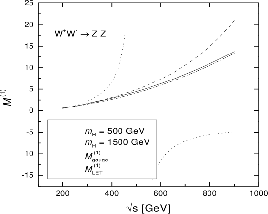
Figure 1: Tree-level amplitudes of the process $WW\to ZZ$ as a function of $\sqrt{s}$ for different values of $m_{H}$. The Higgs boson width, $\Gamma_{H}$, is set to zero, $\cos{\theta_{cm}}=0.5$, $\rho=1$, $m_{Z}=91.2$ GeV, $\sin^{2}{\theta_{W}}=0.231$, $g^{2}=\frac{4\pi\alpha_{em}}{\sin^{2}{\theta_{W}}}\doteq 0.42$.

2.2 $W^{+}(k_{1})+Z(k_{2})\to Z(k_{3})+W^{+}(k_{4})$

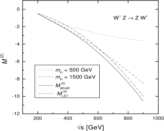
Figure 2: Tree-level amplitudes of the process $WZ\to WZ$.

On the tree-level the pure gauge contributions are from $W$-exchange in $s$ and $t$ channels and the contact graph

$${\cal M}^{(2)}_{kW}=\frac{-g^{2}\cos^{2}{\theta_{W}}}{k-m_{W}^{2}}A^{(2)}_{kW}\quad k=s,t$$ (8)

$${\cal M}^{(2)}_{c}=-g^{2}\cos^{2}{\theta_{W}}A^{(2)}_{c}$$ (9)

The asymptotic behaviour of the complete tree-level gauge amplitude is

$${\cal M}^{(2)}_{gauge} = {\cal M}^{(2)}_{sW}+{\cal M}^{(2)}_{tW}+{\cal M}^{(2)}_{c}$$ (10)

$$= {\cal M}^{(2)}_{LET}-\frac{g^{2}(2x(1-x)+\rho\cos^{2}{\theta_{W}}(3+2x-x^{2}))}{4\rho^{2}\cos^{2}{\theta_{W}}(1-x)}+O\left(\frac{m_{W}^{2}}{s}\right)$$

where a low-energy amplitude is usually defined as

$${\cal M}^{(2)}_{LET}=\frac{g^{2}u}{4\rho m_{W}^{2}}=-\frac{g^{2}s}{8\rho m_{W}^{2}}\,(1+\cos{\theta_{cm}})+O(s^{0})\ .$$

The exchange of the Higgs boson in the $u$-channel

$${\cal M}^{(2)}_{uH}=-g^{2}\frac{m_{W}m_{Z}}{\cos{\theta_{W}}}\frac{(\varepsilon_{1}\cdot\varepsilon^{*}_{4})\,(\varepsilon_{2}\cdot\varepsilon^{*}_{3})}{u-M^{2}_{H}}$$ (11)

has for longitudinal polarizations the high-energy expansion

$${\cal M}^{(2)}_{uH}=\frac{g^{2}\sqrt{\rho}}{8m_{W}^{2}}\,(1+\cos{\theta_{cm}})\,s+O(s^{0})=-\frac{g^{2}\sqrt{\rho}}{4m_{W}^{2}}\,u+O(s^{0})\ .$$

Figure 2 shows complete tree-level amplitude ${\cal M}^{(2)}$ for different $m_{H}$ and compares it with ${\cal M}^{(2)}_{gauge}$ and ${\cal M}^{(2)}_{LET}$.

2.3 $W^{+}(k_{1})+W^{+}(k_{2})\to W^{+}(k_{3})+W^{+}(k_{4})$

Figure 3: Tree-level amplitudes of the process $W^{+}W^{+}\to W^{+}W^{+}$.

On the tree-level graphs with $\gamma$ and $Z$ exchange in $t$ and $u$ channels and contact graph contribute. In the Standard Model, Higgs boson exchange in $t$ and $u$ channels gives the desired high energy behaviour.

$${\cal M}^{(3)}_{kZ}=\frac{-g^{2}\cos^{2}{\theta_{W}}}{k-m_{Z}^{2}}A^{(3)}_{kZ}\qquad{\cal M}^{(3)}_{k\gamma}=\frac{-e^{2}}{k}A^{(3)}_{k\gamma}\qquad k=t,u\ .$$

Because longitudinal term in the $Z$ boson propagator does not contribute we have

$$A^{(3)}_{k\gamma}=A^{(3)}_{kZ}\ .$$

Contact graph amplitude for longitudinally polarized gauge bosons has the form

$${\cal M}^{(3)}_{c}=g^{2}A^{(3)}_{c}=\frac{g^{2}s}{8\,m_{W}^{4}}\,(-8\,m_{W}^{2}+3\,s-s\,\cos^{2}{\theta_{cm}})$$ (12)

The gauge amplitude can be written as

$${\cal M}^{(3)}_{gauge}=-g^{2}\cos^{2}{\theta_{W}}\left[\frac{A^{(3)}_{tZ}}{t-m_{Z}^{2}}+\frac{A^{(3)}_{uZ}}{u-m_{Z}^{2}}\right]-g^{2}\sin^{2}{\theta_{W}}\left[\frac{A^{(3)}_{t\gamma}}{t}+\frac{A^{(3)}_{u\gamma}}{u}\right]+{\cal M}^{(3)}_{c}$$ (13)

Expanding this expression in powers of $s$ gives

$${\cal M}^{(3)}_{gauge}= - g^{2}\cos^{2}{\theta_{W}}\left[\frac{3-\cos^{2}{\theta_{cm}}}{8m_{W}^{4}}\,s^{2}-\frac{3m_{Z}^{2}}{4m_{W}^{4}}\,s+O(s^{0})\right]$$ (14)

$$- g^{2}\sin^{2}{\theta_{W}}\,\left[\frac{3-\cos^{2}{\theta_{cm}}}{8m_{W}^{4}}\,s^{2}+O(s^{0})\right]$$

$$+ g^{2}\left[\frac{3-\cos^{2}{\theta_{cm}}}{8m_{W}^{4}}\,s^{2}-\frac{s}{m_{W}^{2}}\right]$$

Quadratic (in $s$) divergencies are canceled and including constant terms of the order $O(s^{0})$ we get

$${\cal M}^{(3)}_{gauge}={\cal M}^{(3)}_{LET}-g^{2}\,\frac{\left(3+{x^{2}}-\rho\,\cos^{2}{\theta_{W}}(6-4\,{\rho}+10{x^{2}}-12\,{\rho}\,{x^{2}}\right)}{2\,{\rho^{2}}\,\left(1-{x^{2}}\right)\,{\cos^{2}{\theta_{W}}^{2}}}+O\left(\frac{m_{W}^{2}}{s}\right)$$ (15)

where

$${\cal M}^{(3)}_{LET}=-\frac{g^{2}\,s}{4m_{W}^{2}}\left(4-\frac{3}{\rho}\right)\ .$$ (16)

This linear divergence should be canceled by Higgs exchange in $t$ and $u$ channels

$${\cal M}^{(3)}_{H}=-g^{2}m_{W}^{2}\left[\frac{(\varepsilon_{1}\cdot\varepsilon^{*}_{3})(\varepsilon_{2}\cdot\varepsilon^{*}_{4})}{t-m_{H}^{2}}+\frac{(\varepsilon_{1}\cdot\varepsilon^{*}_{4})(\varepsilon_{2}\cdot\varepsilon^{*}_{3})}{u-m_{H}^{2}}\right]$$ (17)

with high-energy expansion

$${\cal M}^{(3)}_{H}=\frac{g^{2}\,s}{4m_{W}^{2}}+O(s^{0})\ .$$ (18)

Comparing (16) and (18) we see that $\rho=1$ ensures desired cancellation.

2.4 $W^{+}(k_{1})+W^{-}(k_{2})\to W^{+}(k_{3})+W^{-}(k_{4})$

Figure 4: Tree-level amplitudes of the process $W^{+}W^{-}\to W^{+}W^{-}$.

In this case we have to consider $Z$, $\gamma$ and Higgs boson exchange in $s$ and $t$ channels and contact graph. As in the previous sections we write

$${\cal M}^{(4)}_{kZ}=\frac{-g^{2}\cos^{2}{\theta_{W}}}{k-m_{Z}^{2}}A^{(4)}_{kZ}\qquad{\cal M}^{(4)}_{k\gamma}=\frac{-e^{2}}{k}A^{(4)}_{k\gamma}\qquad k=s,t$$

The results for the $A$ parts of the amplitude can be obtained directly from corresponding formulae for the process $W^{+}Z\to W^{+}Z$ by setting $m_{Z}=m_{W}$

$$A^{(4)}_{(s,t)(Z,\gamma)}=-A^{(2)}_{(s,t)W}\big{|}_{m_{Z}=m_{W}}$$

or we can also notice that $A^{(4)}_{tZ}=-A^{(3)}_{tZ}$. Again we have $A^{(4)}_{kZ}=A^{(4)}_{k\gamma}$. In the case of longitudinally polarized gauge bosons

$${\cal M}^{(4)}_{c}=g^{2}A^{(4)}_{c}=\frac{g^{2}s}{16\,m_{W}^{4}}\,(8\,m_{W}^{2}-3\,s-24\,m_{W}^{2}\,x+6\,s\,x+s\,x^{2})$$ (19)

Let us examine high-energy expansion of gauge amplitude

$${\cal M}^{(4)}_{gauge}=-g^{2}\cos^{2}{\theta_{W}}\left[\frac{A^{(4)}_{sZ}}{s-m_{Z}^{2}}+\frac{A^{(4)}_{tZ}}{t-m_{Z}^{2}}\right]-g^{2}\sin^{2}{\theta_{W}}\left[\frac{A^{(4)}_{s\gamma}}{s}+\frac{A^{(4)}_{t\gamma}}{t}\right]+{\cal M}^{(4)}_{c}\ .$$ (20)

$${\cal M}^{(4)}_{gauge}=- g^{2}\cos^{2}{\theta_{W}} \left(\frac{x}{4m_{W}^{4}}s^{2}+\frac{m_{Z}^{2}x}{4m_{W}^{4}}s+\frac{x^{2}+2x-3}{16m_{W}^{4}}s^{2}+\frac{3m_{Z}^{2}-16m_{W}^{2}x+m_{Z}^{2}x}{8m_{W}^{4}}s\right)$$

$$- g^{2}\sin^{2}{\theta_{W}} \left(\frac{x}{4m_{W}^{4}}s^{2}+\frac{x^{2}+2x-3}{16m_{W}^{4}}s^{2}-\frac{2x}{m_{W}^{2}}s\right)+O(s^{0})$$

$$+ g^{2} \left(\frac{x^{2}+6x-3}{16m_{W}^{4}}s^{2}+\frac{1-3x}{2m_{W}^{2}}s\right)$$ (21)

After simplification and including terms of order $O(s^{0})$ we get

$${\cal M}^{(4)}_{gauge} = {\cal M}^{(4)}_{LET}$$

$$+ g^{2}\frac{(3+x^{2}-\rho\,\cos^{2}{\theta_{W}}(12-12\,\rho+12\,x-16\,\rho\,x-8\,x^{2}+12\,\rho\,x^{2}))}{4\,\rho^{2}\,(1-x)\,\cos^{2}{\theta_{W}}}$$

$$+ O\left(\frac{m_{W}^{2}}{s}\right)$$

where as in the case of the process #1 I denote

$${\cal M}^{(4)}_{LET}=-\frac{g^{2}u}{4m_{W}^{2}}\left(4-\frac{3}{\rho}\right)$$

in accordance with [LET]. High-energy expansion of the Higgs boson contribution

$${\cal M}^{(4)}_{H}=-g^{2}M^{2}_{W}\left[\frac{(\varepsilon_{1}\cdot\varepsilon_{2})(\varepsilon_{3}^{*}\cdot\varepsilon_{4}^{*})}{s-m_{H}^{2}}+\frac{(\varepsilon_{1}\cdot\varepsilon_{3}^{*})(\varepsilon_{2}^{*}\cdot\varepsilon_{4}^{*})}{t-m_{H}^{2}}\right]$$ (22)

is

$${\cal M}^{(4)}_{H}=-\frac{g^{2}s}{8m_{W}^{2}}(1+\cos{\theta_{cm}})+O(s^{0})=\frac{g^{2}u}{4m_{W}^{2}}+O(s^{0})$$

Appendix A Exact formulae

The following Feynman rules and notation is used (all momenta are outgoing) [horejsi]
{\begin{picture}(171.0,174.0)\put(10.0,10.0){}\put(12.35,9.93){}} \put(12.35,9.93){}