Effective QCD coupling and power corrections
to photon-photon scattering

Abstract

The scattering of two off-shell photons is an infrared-safe process in QCD. For photon virtualities $Q$ in the range of a few GeV, accessible at LEPII, power-behaved contributions in $(\Lambda_{\rm{QCD}}/Q)^{n}$ to the total cross section may become non-negligible. Based on a dispersion relation for the running coupling, we discuss these contributions and calculate the coefficients of the leading power correction for transversely polarized and longitudinally polarized virtual photons.

Two-photon collisions provide one of the dominant modes in experiments at high-energy $e^{\pm}e^{-}$ colliders. If the photons are sufficiently far off shell, the process is dominated by short-distance QCD interactions. A survey of the QCD studies in photon-photon scattering that are currently being carried out at LEPII may be found in Ref. [1]. In particular, the total cross section for scattering two off-shell photons is an infrared-safe observable. The role of this property has recently been emphasized in the context of investigations of the high-energy limit of QCD [2]. Predictions for $\sigma(\gamma^{*}\,\gamma^{*})$ can be computed in perturbation theory and tested as a function of the photon virtualities. For virtualities $Q$ of the order of a few GeV, contributions to $\sigma$ suppressed by powers of $\Lambda_{\rm{QCD}}/Q$ may become non-negligible. These contributions are the subject of this paper.

A systematic approach to the calculation of power-behaved corrections to hard processes is an open problem in QCD. For cases in which an operator product expansion is applicable, this provides a general framework to classify higher-twist contributions. However, so far this has proved to be of only limited practical use. On the other hand, there have been efforts to develop methods that allow one to derive estimates of power corrections to a given observable from the study of the infrared behavior of its perturbative series [3]. In this context different techniques have been proposed over the past few years and applied to a variety of hard processes (for recent reviews see, for instance, Ref. [4]). The basic observation underlying these methods is that the factorial growth of the coefficients of the QCD perturbation series in large orders gives rise to ambiguities in the perturbative predictions which are proportional to power-behaved contributions. These ambiguities can be interpreted as being due to an artificial separation between short-distance and long-distance physics in the perturbative treatment. From the requirement that they must cancel in the physical cross sections once higher orders as well as nonperturbative contributions are included, one is able to derive information on the structure of the power correction.

The physical origin of these power-like contributions is an infrared one. They are associated with the loop integrations over the regions of small momenta in Feynman graphs. Based on this, the authors of Refs. [5, 6] have proposed a dispersion relation for the QCD running coupling in order to relate power-like corrections to the behavior of the coupling at small momentum scales. In this paper, we will use this dispersion relation to analyze the exchange of gluons in high-energy photon-photon interactions. This will enable us to identify the leading power correction to the total photon-photon cross section.

We will discuss the scattering of two off-shell (spacelike) photons with momenta $q_{A}$ and $q_{B}$, $\gamma^{*}(q_{A})+\gamma^{*}(q_{B})\to{\mbox{hadrons}}$, with the virtualities $q_{A}^{2}\equiv-Q^{2}_{A}$ and $q_{B}^{2}\equiv-Q^{2}_{B}$ being large compared to $\Lambda_{\rm{QCD}}^{2}$. We will focus on the region where the center-of-mass energy $\sqrt{s}\equiv\sqrt{(q_{A}+q_{B})^{2}}$ is much larger than $Q_{A}$ and $Q_{B}$. In this region questions related to power-like corrections become especially important, because power-like corrections are expected to be associated with the mechanism that unitarizes the total cross section at asymptotic energies. We will thus start with the large-$s$ form of the perturbative cross section, in which terms that fall like $Q^{2}/s$ are neglected. In the Born approximation, the corresponding amplitude is given by graphs with exchange of one gluon between two quark-antiquark pairs created by the virtual photons (Fig. 1). In this approximation the total cross section has the structure [2]

$$\sigma_{0}(s,Q_{A}^{2},Q_{B}^{2})={1\over{2\,\pi}}\,\int\,{{d^{2}\,{\mbox{\bf k}}}\over{\pi}}\,{1\over{({{\mbox{\bf k}}}^{2})^{2}}}\,G({\mbox{\bf k}}^{2},Q^{2}_{A})\,G({\mbox{\bf k}}^{2},Q^{2}_{B})\;\;\;\;.$$ (1)

Here $d^{2}{{\mbox{\bf k}}}$ denotes the integration over the transverse momentum flowing in the gluon line. The factors $1/\left({{\mbox{\bf k}}}^{2}\right)^{2}$ come from the gluon propagators. The factors $G$ are each proportional to $\alpha_{s}$,

$$G=\alpha_{s}\,g({{\mbox{\bf k}}}^{2}/Q^{2})\;\;\;,$$ (2)

and describe the coupling of the gluon to the $q\,{\bar{q}}$ system. The explicit form of the functions $g({{\mbox{\bf k}}}^{2}/Q^{2})$ depends on the photon polarization. In what follows we will discuss first the cross section averaged over the two transverse polarizations and then we will extend our results to the case of the longitudinal polarization.

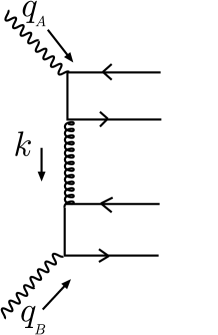
FIG. 1.: One of the graphs contributing to the Born amplitude for the process $\gamma^{*}+\gamma^{*}\to{\mbox{hadrons}}$ at large $s$.

The cross section $\sigma_{0}$ has a scaling behavior in the photon virtualities of the type $\sigma\propto 1/Q^{2}$, modulated by logarithmic scaling-violation factors in the ratio of the two virtualities. To evaluate the corrections to this behavior that are suppressed by powers of the photon virtualities, we begin by introducing the running coupling $\alpha_{s}({\mbox{\bf k}}^{2})$ for each one of the factors $G$ in the integral (1). Following the method of Refs. [5, 6], we consider the dispersive representation of the QCD coupling in terms of the spectral density $\rho_{s}$,

$$\alpha_{s}({\mbox{\bf k}}^{2})=-\int_{0}^{\infty}\,{{d\,\mu^{2}}\over{\mu^{2}+{\mbox{\bf k}}^{2}}}\,\rho_{s}(\mu^{2})\;\;\;\;,$$ (3)

and we define the effective coupling $\alpha_{{\rm{eff}}}$ according to the relation

$$\rho_{s}(\mu^{2})={{\partial}\over{\partial\,\ln\mu^{2}}}\alpha_{{\rm{eff}}}(\mu^{2})\;\;\;\;.$$ (4)

We thus have

$$\alpha_{s}({\mbox{\bf k}}^{2})={\mbox{\bf k}}^{2}\,\int_{0}^{\infty}\,{{d\,\mu^{2}}\over{({\mbox{\bf k}}^{2}+\mu^{2})^{2}}}\,\alpha_{{\rm{eff}}}(\mu^{2})\;\;\;\;.$$ (5)

The effective coupling $\alpha_{{\rm{eff}}}$ differs from the perturbative coupling in the infrared region. The form of $\alpha_{{\rm{eff}}}$ is determined by nonperturbative physics. As we shall see, the main point of this approach is that, if this form can be assumed to be universal, then power-behaved contributions to the cross section can be parametrized in terms of moments of the effective coupling variation at low transverse momentum scales.

Replacing the strong coupling in Eq. (1) by Eq. (5) yields

$$\sigma={1\over{2\,\pi}}\,\int_{0}^{\infty}\,{{d\,\mu^{2}_{A}}\over{\mu^{2}_{A}}}\,\alpha_{{\rm{eff}}}(\mu^{2}_{A})\,\int_{0}^{\infty}\,{{d\,\mu^{2}_{B}}\over{\mu^{2}_{B}}}\,\alpha_{{\rm{eff}}}(\mu^{2}_{B})\,{\phi}(Q_{A}^{2},Q_{B}^{2};\mu^{2}_{A},\mu^{2}_{B})\;\;\;\;,$$ (6)

with the function ${\phi}$ being given by

$${\phi}(Q_{A}^{2},Q_{B}^{2};\mu^{2}_{A},\mu^{2}_{B})=\mu^{2}_{A}\,\mu^{2}_{B}\,\int_{0}^{\infty}\,{{d\,{{\mbox{\bf k}}}^{2}}\over{({\mbox{\bf k}}^{2}+\mu^{2}_{A})^{2}\;({\mbox{\bf k}}^{2}+\mu^{2}_{B})^{2}}}\,\,g({{\mbox{\bf k}}}^{2}/{Q}^{2}_{A})\,g({{\mbox{\bf k}}}^{2}/{Q}^{2}_{B})\;\;\;\;.$$ (7)

Eq. (6) is written in terms of two dispersion variables $\mu_{A}$, $\mu_{B}$, corresponding to the fact that our starting amplitude (Fig. 1) is a two-loop contribution in QCD. Introducing the variation $\delta\alpha_{{\rm{eff}}}$ of the strong coupling at low scales, we decompose $\alpha_{{\rm{eff}}}$ as follows

$$\alpha_{{\rm{eff}}}(\mu^{2})=\alpha_{\rm{PT}}(\mu^{2})+\delta\alpha_{{\rm{eff}}}(\mu^{2})\hskip 14.22636pt,$$ (8)

where $\alpha_{\rm{PT}}$ denotes the form of the coupling in perturbation theory. The decomposition (8) gives rise to terms in $\alpha_{\rm{PT}}\times\alpha_{\rm{PT}}$, $\alpha_{\rm{PT}}\times\delta\alpha_{{\rm{eff}}}$, and $\delta\alpha_{{\rm{eff}}}\times\delta\alpha_{{\rm{eff}}}$ in Eq. (6).

The integration of the terms in $\alpha_{\rm{PT}}\times\alpha_{\rm{PT}}$ is dominated by values of the dispersion variables of the order of the hard scales, $Q_{A}$ and $Q_{B}$, as we will see below. Thus, these terms give rise to the standard leading result for the cross section in perturbation theory. The terms involving $\delta\alpha_{{\rm{eff}}}$, on the other hand, probe the behavior of the function $\phi$ at small values of the dispersion variables, because the distribution of $\delta\alpha_{{\rm{eff}}}$ is concentrated at small scales. These terms are responsible for power-behaved corrections to $\sigma$. We will see that in the case of the leading power correction the quadratic term in $\delta\alpha_{{\rm{eff}}}$ does not contribute and the correction comes entirely from the linear term in $\delta\alpha_{{\rm{eff}}}$.

To study the form of the function $\phi$ at small $\mu^{2}$, we use the explicit expression for $g$. For transversely polarized photons, this is given by [2]

$$g({{\mbox{\bf k}}}^{2}/Q^{2})=8\,\alpha\,\left(\sum_{q}e^{2}_{q}\right)\,\int_{0}^{1}\,{d\,z}\,P(z)\,\int_{0}^{1}\,{d\,\lambda}\,P(\lambda)\,{{\,{{\mbox{\bf k}}}^{2}\,}\over{\lambda\,(1-\lambda)\,{{\mbox{\bf k}}}^{2}+z\,(1-z)\,Q^{2}}}\hskip 14.22636pt,$$ (9)

where $\alpha$ is the electromagnetic fine structure, $e_{q}$ is the quark electric charge in units of $e=\sqrt{4\,\pi\,\alpha}$, and $P$ is the vector $\to$ fermion splitting function

$$P(x)={{x^{2}+(1-x)^{2}}\over 2}\hskip 14.22636pt.$$ (10)

From Eqs. (7) and (9) we may observe that for small $\mu$ the function $\phi$ vanishes. This is associated with the fact that the $\gamma^{*}\,\gamma^{*}$ cross section is an infrared safe quantity in perturbation theory (see Eq. (1)), that is, the factors $g$ vanish like ${{\mbox{\bf k}}}^{2}/Q^{2}$ (times logarithms) as ${{\mbox{\bf k}}}^{2}\to 0$. For large $\mu$ the function $\phi$ also vanishes. This is associated with the fact that the graph in Fig. 1 is well-behaved in the ultraviolet, that is, the factors $g$ do not grow more than logarithmically at large ${{\mbox{\bf k}}}^{2}$.

FIG. 2.: The dependence of the function $\phi$ on one of the dispersion variables ($\mu_{B}$) for different values of the other one ($\mu_{A}$). We take $Q_{A}=Q_{B}$ and plot the rescaled function $\Phi=Q_{A}\,Q_{B}\,\phi/(8\,\alpha\,\sum_{q}e_{q}^{2})^{2}$ versus $\mu_{B}^{2}/(Q_{A}\,Q_{B})$.

We now evaluate the function $\phi$ numerically. In Fig. 2 we plot the $\mu_{B}$-dependence of the dimensionless function $Q_{A}\,Q_{B}\,\phi$ for fixed (small) values of $\mu_{A}$, working at $Q_{A}=Q_{B}$. First, we note that $\phi$ peaks in the region where the ratio $\mu_{A}/\mu_{B}$ of the dispersion variables is of order $1$ and their product is of order $Q_{A}\,Q_{B}$. Then the leading contribution to the term $\alpha_{\rm{PT}}\times\alpha_{\rm{PT}}$ from the integral (6) is obtained by pulling out of the integral the factors of $\alpha_{\rm{PT}}$ evaluated at a scale of order $Q_{A}\,Q_{B}$. We thus recover the leading perturbative result (1). Second, we consider the term $\delta\alpha_{{\rm{eff}}}(\mu_{A}^{2})\,\alpha_{\rm{PT}}(\mu_{B}^{2})$. We see from Fig. 2 that for small $\mu_{A}$ the function $\phi$ peaks at a value ${\overline{\mu}}_{B}^{2}$ proportional to $\sqrt{Q_{A}\,Q_{B}}$ and to $\sqrt{\mu_{A}^{2}}$. Then we approximately perform the $\mu_{B}^{2}$-integration by pulling out of the integral the factor of $\alpha_{\rm{PT}}$ evaluated at the scale ${\overline{\mu}}_{B}^{2}$ and computing the integral of $\phi$. By adding the symmetric term with $\mu_{A}$ and $\mu_{B}$ interchanged, we write the contribution $\sigma_{1}$ from the terms of the first order in $\delta\alpha_{{\rm{eff}}}$ as

$$\sigma_{1}\simeq{1\over{\pi}}\,\int_{0}^{\infty}\,{{d\,\mu^{2}_{A}}\over{\mu^{2}_{A}}}\,\delta\alpha_{{\rm{eff}}}(\mu^{2}_{A})\;\alpha_{{\rm{PT}}}\left(Q_{A}\,Q_{B}\,\sqrt{\mu^{2}_{A}/(Q_{A}\,Q_{B})}\right)\;{\widetilde{\phi}}(Q_{A}^{2},Q_{B}^{2};\mu^{2}_{A})\;\;\;\;,$$ (11)

where the function ${\widetilde{\phi}}$ is defined as

$${\widetilde{\phi}}=\int_{0}^{\infty}\,{{d\,\mu^{2}_{B}}\over{\mu^{2}_{B}}}\,\phi\;\;\;\;.$$ (12)

Next we use the fact that the requirement of consistency with the operator product expansion [7] constrains the structure of the effective coupling variation $\delta\alpha_{{\rm{eff}}}$ [6, 8]. Let us define the moments

$$A^{(n)}_{2\,p}={1\over{2\,\pi}}\,{{d^{n}}\over{dp^{n}}}\,\int_{0}^{\infty}\,{{d\,\mu^{2}}\over\mu^{2}}\,\left(\mu^{2}\right)^{p}\,\delta\alpha_{{\rm{eff}}}(\mu^{2})\,\;\;\;.$$ (13)

In order that the ultraviolet behavior of the running coupling be not ruined by the variation $\delta\alpha_{{\rm{eff}}}$, the moments with $n=0$ and $p$ integer have to vanish [6, 8, 9]. This implies that only terms in ${\widetilde{\phi}}$ that are nonanalytic in $\mu_{A}^{2}$ for small $\mu_{A}^{2}$ can contribute to power corrections. To find these terms, we examine the dominant region of integration in Eq. (7), $\mu_{A}^{2}{\raisebox{-1.72218pt}{\hbox to0.0pt{$\,\sim\,$\hss}}\raisebox{1.72218pt}{$\,<\,$}}{\bf k}^{2}{\raisebox{-1.72218pt}{\hbox to0.0pt{$\,\sim\,$\hss}}\raisebox{1.72218pt}{$\,<\,$}}Q_{A}\,Q_{B}$. By evaluating the contribution from this region, we obtain the following approximate expression for the function ${\widetilde{\phi}}$:

$${\widetilde{\phi}}(Q_{A}^{2},Q_{B}^{2};\mu^{2}_{A})\simeq\left(8\,\alpha\,\sum_{q}e_{q}^{2}\right)^{2}\,{1\over{Q_{A}\,Q_{B}}}\,(-\eta)\,\left\{{2\over 9}\,{\mbox{Li}}_{3}(-{1\over\eta})+{1\over 27}\,{\mbox{Li}}_{2}(-{1\over\eta})\right.$$ (14)

$$\left.+\left[{35\over 324}+{1\over 36}\,\ln^{2}\left({Q_{A}^{2}\over Q_{B}^{2}}\right)\right]\,\ln\left({{1+\eta}\over\eta}\right)+\left[{49\over 324}-{1\over 36}\,\ln^{2}\left({Q_{A}^{2}\over Q_{B}^{2}}\right)\right]\,{1\over{1+\eta}}\right\}\hskip 5.69046pt,\hskip 11.38092pt\eta\equiv{\mu^{2}_{A}\over{Q_{A}\,Q_{B}}}\hskip 5.69046pt,$$ (15)

where

$${\mbox{Li}}_{2}(z)=-\int_{0}^{z}\,{{dt}\over t}\,\ln(1-t)\hskip 17.07182pt,\hskip 34.14322pt{\mbox{Li}}_{3}(z)=\int_{0}^{z}\,{{dt}\over t}\,{\mbox{Li}}_{2}(t)\hskip 17.07182pt.$$ (16)

This formula is accurate up to the leading power in $\eta=\mu^{2}_{A}/(Q_{A}\,Q_{B})$ and up to the single logarithms. Higher powers in $\eta$ as well as constants associated with the leading power are changed by the terms that we have dropped in performing the integral (7). To determine the nonanalytic behavior that controls the leading power correction to $\sigma$ we expand around $\eta=0$:

$${\widetilde{\phi}}(Q_{A}^{2},Q_{B}^{2};\mu^{2}_{A})\simeq\left(8\,\alpha\,\sum_{q}e_{q}^{2}\right)^{2}\,{1\over{Q_{A}\,Q_{B}}}\,{1\over 27}\,\eta\,\left\{\ln^{3}{1\over\eta}+{1\over 2}\,\ln^{2}{1\over\eta}\right.$$ (17)

$$+\left.\left[6\,\zeta(2)-{35\over 12}-{3\over 4}\,\ln^{2}\left({Q_{A}^{2}\over Q_{B}^{2}}\right)\right]\,\ln{1\over\eta}+\{{\mbox{analytic}}\;{\mbox{terms}}\}\right\}+{\cal O}(\eta^{2})\hskip 5.69046pt,\hskip 5.69046pt\zeta(2)\simeq 1.64\hskip 2.84544pt.$$ (18)

Thus, from Eqs. (11) and (13) we find

$$\sigma_{1}\simeq{{\left(8\,\alpha\,\sum e_{q}^{2}\right)^{2}\,2\,\alpha_{\rm{PT}}(Q_{A}Q_{B})}\over{27\,Q_{A}^{2}\,Q_{B}^{2}}}\,\left[-(3L^{2}+L+k)A^{(1)}_{2}+\left(3\,L+{1\over 2}\right)A^{(2)}_{2}-A^{(3)}_{2}\right]$$ (19)

where

$$L=\ln(Q_{A}Q_{B})\;\;,\;\;\;\;\;k=6\,\zeta(2)-{35\over 12}-{3\over 4}\,\ln^{2}\left({Q_{A}^{2}\over Q_{B}^{2}}\right)\;\;.$$ (20)

Here we have written $\alpha_{\rm{PT}}(Q_{A}Q_{B}\sqrt{\eta})=\alpha_{\rm{PT}}(Q_{A}Q_{B})+{\cal O}(\alpha^{2}_{\rm{PT}}\,\ln\eta)$ and neglected the higher order term on the right-hand side. In the definition of $L$ in Eq. (20) we have implicitly taken the scale in the logarithm to be $1\,{\mbox{GeV}}^{2}$.

Eq. (19) gives the result for the leading power correction to the $\gamma^{*}\,\gamma^{*}$ cross section in terms of the dimensionful nonperturbative parameters $A_{2}^{(i)}$. These parameters are thought of as being universal and should be determined by fits to experimental data. The coefficients of these parameters are given in Eq. (19) up to terms that vanish like $Q^{2}/s$ at large $s$. We see that the contributions in $A^{(1)}_{2}$ and $A^{(2)}_{2}$ are enhanced by double and single logarithms of the hard scale $Q_{A}\,Q_{B}$.

So far, there have been attempts to study the nonperturbative moments $A^{(i)}_{2}$ based on data for deeply inelastic lepton-nucleon scattering and for hadronic final states in $e^{+}\,e^{-}$ annihilation. Data on the structure function $F_{2}$ suggest that $A^{(1)}_{2}\,\simeq-0.15\,{\mbox{GeV}}^{2}$ [10]. Very little is known about $A^{(2)}_{2}$ and $A^{(3)}_{2}$ at present. $A^{(2)}_{2}$ enters in the power correction to the mean value of the three-jet resolution in $e^{+}\,e^{-}$ annihilation. A recent analysis of data recorded at PETRA suggests that this correction should be very small [11]. Assuming that the contribution of $A^{(1)}_{2}$ predominates in Eq. (19), owing to its enhanced coefficient, we expect the leading power correction to be positive.

To complete our analysis, we need to show that, as anticipated, the term of the second order in $\delta\alpha_{{\rm{eff}}}$ in Eq. (6) does not contribute to the leading power correction. We write this term as

$$\sigma_{2}={1\over{2\,\pi}}\,\int_{0}^{\infty}\,{{d\,\mu^{2}_{A}}\over{\mu^{2}_{A}}}\,\delta\alpha_{{\rm{eff}}}(\mu^{2}_{A})\,\int_{0}^{\infty}\,{{d\,\mu^{2}_{B}}\over{\mu^{2}_{B}}}\,\delta\alpha_{{\rm{eff}}}(\mu^{2}_{B})\,{\phi}\;\;\;\;.$$ (21)

This contribution probes the function $\phi$ in the corner of the phase space where both $\mu^{2}_{A}$ and $\mu^{2}_{B}$ are small. We may restrict the ${{\mbox{\bf k}}}^{2}$-integration in Eq. (7) to the region ${{\mbox{\bf k}}}^{2}{\raisebox{-1.72218pt}{\hbox to0.0pt{$\,\sim\,$\hss}}\raisebox{1.72218pt}{$\,<\,$}}Q^{2}$, with $Q^{2}$ being of the order of the hard scales $Q_{A}^{2}$, $Q_{B}^{2}$, and we may rewrite the function $\phi$ as a sum of two pieces, each proportional to a logarithmic derivative with respect to one of the dispersion variables:

$${\phi}(Q_{A}^{2},Q_{B}^{2};\mu^{2}_{A},\mu^{2}_{B})\simeq -{\partial\over{\partial\ln\mu^{2}_{A}}}\left[{\mu^{2}_{B}\over{(\mu^{2}_{A}-\mu^{2}_{B})^{2}}}\,\int_{0}^{Q^{2}}\,{{d\,{{\mbox{\bf k}}}^{2}}\over{{\mbox{\bf k}}^{2}+\mu^{2}_{A}}}\,\,g({{\mbox{\bf k}}}^{2}/{Q}^{2}_{A})\,g({{\mbox{\bf k}}}^{2}/{Q}^{2}_{B})\right]$$ (23)

$$-{\partial\over{\partial\ln\mu^{2}_{B}}}\left[{\mu^{2}_{A}\over{(\mu^{2}_{A}-\mu^{2}_{B})^{2}}}\,\int_{0}^{Q^{2}}\,{{d\,{{\mbox{\bf k}}}^{2}}\over{{\mbox{\bf k}}^{2}+\mu^{2}_{B}}}\,\,g({{\mbox{\bf k}}}^{2}/{Q}^{2}_{A})\,g({{\mbox{\bf k}}}^{2}/{Q}^{2}_{B})\right]\;.$$

The pole at $\mu^{2}_{A}=\mu^{2}_{B}$ cancels in the sum of the two pieces. This may be checked, for instance, by substituting the expression for $g$, expanding it for small ${\mbox{\bf k}}^{2}$ and performing the integrals explicitly. Taking this cancellation into account, the first piece gives rise to terms that are analytic in $\mu^{2}_{B}$ and possibly have nonanalytic contributions in $\mu^{2}_{A}$. Analogously, the second piece gives rise to terms that are analytic in $\mu^{2}_{A}$ and possibly have nonanalytic contributions in $\mu^{2}_{B}$. Since, as already noted, integer moments of $\delta\alpha_{{\rm{eff}}}$ vanish, for each term we get a vanishing contribution in Eq. (21) from either the integral in $\mu^{2}_{A}$ or the integral in $\mu^{2}_{B}$. Therefore, $\sigma_{2}$ does not contribute to the leading power correction.

Finally, let us consider the scattering of longitudinally polarized photons. The function $g^{(L)}$ for this case has a structure analogous to Eq. (9) but with a different splitting function, $P^{(L)}$ [2]. The longitudinal splitting function vanishes at the endpoints:

$$P^{(L)}=\sqrt{2}\,x\,(1-x)\hskip 11.38092pt.$$ (24)

This can be seen as being associated with the absence of aligned-jet terms for longitudinal photon scattering at high energies [12]. As a result, by performing a calculation analogous to the one described above for the transverse case, we find that the small-$\eta$ expansion of ${\widetilde{\phi}}^{(L)}$ has at most single logarithms:

$${\widetilde{\phi}}^{(L)}(Q_{A}^{2},Q_{B}^{2};\eta)\simeq\left(8\,\alpha\,\sum_{q}e_{q}^{2}\right)^{2}\,{1\over{Q_{A}\,Q_{B}}}\,{1\over 9}\,\eta\,\left[\ln{1\over\eta}+\{{\mbox{analytic}}\;{\mbox{terms}}\}\right]+{\cal O}(\eta^{2})\hskip 17.07182pt.$$ (25)

Therefore, for the power correction to the longitudinal $\gamma^{*}\,\gamma^{*}$ cross section $\sigma^{(L)}$ we get

$$\sigma_{1}^{(L)}\simeq{{\left(8\,\alpha\,\sum e_{q}^{2}\right)^{2}\,2\,\alpha_{\rm{PT}}(Q_{A}Q_{B})}\over{9\,Q_{A}^{2}\,Q_{B}^{2}}}\,\left(-\,A^{(1)}_{2}\right)\hskip 17.07182pt.$$ (26)

We observe that the structure of the power correction is considerably more complicated in the transverse case. In the longitudinal case, the power correction only depends on one nonperturbative moment, $A^{(1)}_{2}$. Moreover, in the longitudinal case the coefficient is not enhanced by logarithms of $Q_{A}\,Q_{B}$. For both transverse and longitudinal scattering, it would be interesting to use experimental data for studying the moments $A^{(i)}_{2}$ and for testing the dispersive structure of the power-behaved terms.

I greatly benefited from discussions with Yu. Dokshitzer, D. Soper and B. Webber. I thank the High Energy Theory group at Brookhaven National Laboratory, the RIKEN-BNL Research Center and the organizers of the RIKEN Workshop on Perturbative QCD for hospitality and support while part of this work was being done. This research was partially funded by the US Department of Energy grant DE-FG03-96ER40969.

REFERENCES

• [1] D.J. Miller, summary talk at the conference Photon97, Egmond-aan-Zee, The Netherlands, 10-15 May 1997, e-print archive hep-ex/9708002.
• [2] S.J. Brodsky, F. Hautmann and D.E. Soper, Phys. Rev. Lett. 78, 803 (1997); preprint SLAC-PUB-7480, e-print archive hep-ph/9706427; preprint SLAC-PUB-7601, e-print archive hep-ph/9707444.
• [3] A.H. Mueller, Nucl. Phys. B250, 327 (1985), Phys. Lett. B 308, 355 (1993), in Proceedings of the Workshop “QCD 20 years later”, Aachen, June 1992, edited by P.M. Zerwas and H.A. Kastrup (World Scientific, Singapore, 1993), p. 162; V.I. Zakharov, Nucl. Phys. B385, 452 (1992).
• [4] M. Beneke, talk at the 5th International Workshop on Deep Inelastic Scattering and QCD, Chicago, IL, 14-18 April 1997, e-print archive hep-ph/9706457; V.M. Braun, talk at the 5th International Conference on Physics beyond the Standard Model, Balholm, Norway, 29 April-4 May 1997, e-print archive hep-ph/9708386.
• [5] Yu.L. Dokshitzer and B.R. Webber, Phys. Lett. B 352, 451 (1995).
• [6] Yu.L. Dokshitzer, G. Marchesini and B.R. Webber, Nucl. Phys. B469, 93 (1996).
• [7] M.A. Shifman, A.I. Vainshtein and V.I. Zakharov, Nucl. Phys. B147, 385 (1979).
• [8] M. Beneke, V.M. Braun and V.I. Zakharov, Phys. Rev. Lett. 73, 3058 (1994).
• [9] P. Ball, M. Beneke and V.M. Braun, Nucl. Phys. B452, 563 (1995).
• [10] M. Dasgupta and B.R. Webber, Phys. Lett. B 382, 273 (1996).
• [11] P.A. Movilla Fernandez et al., preprint PITHA 97/27, e-print archive hep/ex-9708034.
• [12] J.D. Bjorken and J. Kogut, Phys. Rev. D 8, 1341 (1973); L.L. Frankfurt and M. Strikman, Phys. Rep. 160, 235 (1988).