Chapter 1 HADRONIC PHYSICS FROM THE LATTICE

Theoretical Physics Division, Department of Mathematical Sciences,
University of Liverpool, L69 3BX, UK

1.1 INTRODUCTION

Topics covered in this review are the lattice gauge theory approach to the evaluation of non-perturbative hadronic interactions from first principles, particularly applications to glueballs, inter-quark potentials, the running coupling constant and hybrid mesons. Also discussed are the limitations of the quenched approximation.

The theory of the strong interactions is accurately provided by Quantum Chromodynamics (QCD). The theory is defined in terms of elementary components: quarks and gluons. The only free parameters are the quark mass values (apart from an overall energy scale imposed by the need to regulate the theory). This formulation is essentially the unique candidate for the theory of the strong interactions. The only feasible way to describe a departure from QCD would be in terms of quark and gluon substructure. At least at the energy scales up to which it is tested, there is no evidence for such substructure.

QCD provides a big challenge to theoretical physicists. It is defined in terms of quarks and gluons but the physical particles are composites: the mesons and baryons. Any complete description must then yield these bound states: this requires a non-perturbative approach. One can see the limitations of a perturbative approach by considering the vacuum: this will be approximated in perturbation theory as basically empty with rare quark or gluon loop fluctuations. Such a description will allow quarks and gluons to propagate essentially freely which is not the case experimentally. The true (non-perturbative) vacuum can be better thought of as a disordered medium with whirlpools of colour on different scales. Such a non-perturbative treatment then has the possibility to explain why quarks and gluons do not propagate (i.e. quark confinement). Furthermore it will be able to explore other situations than experiment — different quark masses, etc. My notation is that there are $N_{f}$ flavours of light quark with $N$ colours.

Any mathematically precise description of QCD must introduce some regularisation of the ultra-violet divergences. Any such regularisation may spoil the symmetries, for example 4-dimensional Lorentz invariance is broken by dimensional regularisation. Introducing a space time lattice likewise breaks Lorentz invariance. Using a space time lattice with exact gauge invariance retained proves to be a very successful regularisation. In the continuum limit, as the lattice spacing is reduced to zero, Lorentz invariance will be found to be restored.

For a general review of lattice gauge theory, see standard textbooks[1]. Here I give a brief introduction to the salient points. The simplest discretisation of space-time is that introduced by Wilson[2]. Space-time is replaced by a discrete grid (the lattice) but gauge invariance is retained exactly. Then gluonic colour fields which relate the colour coordinate system at different space time points will be represented as links on this lattice. Thus a link of the lattice from $x$ to $x+a$ in the $\mu$-direction (with unit vector $e_{\mu}$) is represented by a $N\times N$ colour matrix which can be thought of as the path-ordered exponential of the continuum colour fields $A_{\mu}(x)$,

$$U_{\mu}(x)\approx e^{igaA_{\mu}(x+{1\over 2}ae_{\mu})}.$$ (1.1)

From these link matrices, the simplest non-trivial gauge invariant is the trace of the path-ordered product of links around a unit square: the plaquette.

$$S_{\Box}={1\over N}{\rm ReTr}(\prod U).$$ (1.2)

Note that, with this definition, a cold lattice with $A\approx 0$ will have all link matrices $U\approx 1$ and hence have $S_{\Box}\approx 1$ , while a hot lattice with random $U$ will have $S_{\Box}\approx 0$. This gauge invariant $S_{\Box}$, when summed over all space-time, is the simplest candidate for the gluonic component of the action: the Wilson gauge action. This follows since naively (i.e. neglecting quantum fluctuations) as $a\to 0$

$$\beta\sum_{\rm hypercube}S_{\Box}-1\ \to\ -{1\over 4}\int F_{\mu\nu}F_{\mu\nu}\,d^{4}x$$ (1.3)

where $\beta=2N/g^{2}$.

Using periodic boundary conditions in space and time, the system will have a finite number of degrees of freedom: the gluon and quark fields at the lattice sites. This finite number of degrees of freedom implies that the theory is a quantum many-body problem rather than a field theory. The step which makes this many-body problem tractable is to consider Euclidean time. With the Euclidean time approach, the formulation of QCD (consider, for example, the functional integral over the gauge fields) is converted into a multiple integral which is well defined mathematically and has a positive definite integrand:

$${\cal Z}=\int DUe^{\beta\sum S_{\Box}},$$ (1.4)

where the integral is over the group manifold of $SU(N)$ of colour for each link matrix $U$. Because of gauge invariance not all links are independent, but integrating over the dependent links only introduces a finite constant which is irrelevant. For a lattice of $L^{4}$ sites with a colour gauge group of SU(3), this would be a $8\times 4\times L^{4}$ dimensional integral (8 from the colour group manifold, $4L^{4}$ from the gauge fields on each link). For any reasonable value of $L$, this is a very high dimension indeed. Simpson’s rule is not the way forward! Because the integrand is positive definite, the standard approach is to use a Monte Carlo approximation to the integrand. This is implemented in an ‘importance sampling’ version so that a stochastic estimate of the integral is made from a finite number of samples (called configurations) of equal weight. The construction of efficient algorithms to achieve this is a topic in itself. Here I will concentrate on the analysis of the outcome, assuming that such configurations have been generated.

So what is at our disposal is a set of samples of the vacuum. It is then straightforward to evaluate the average of various products of fields over these samples — this gives the Green functions by definition. The Green function can then be continued from Euclidean to Minkowski time (in most cases this is trivial) and compared to experiment. Thus masses and matrix elements can be evaluated readily. Scattering, hadronic decays, real-time processes etc will not be directly accessible.

A simple example of a lattice measurement is that of a Wilson loop. This is the expectation value in the vacuum of the path ordered product of links around a closed loop. For example, a rectangular loop of size $R\times T$ can be used to extract the potential between heavy quarks and thus to explore confinement.

So far I have concentrated on the gluonic degrees of freedom of QCD, where an elegant formulation was available. In contrast, the inclusion of quarks in a lattice approach is very inelegant and computationally challenging. The quarks will be represented by Grassmannian variables $\psi$ and the fermionic action for each species of quark will be bilinear $\bar{\psi}Q(m,U)\psi$ where $Q$ is the fermionic matrix for a quark of mass $m$ in the gauge fields $U(x)$, namely $\not{\!\!D}+m$ in the continuum. Various discretisations of this have been proposed. They all have the feature that each fermionic species needs to be at least doubled in a local lattice formulation. The Wilson fermionic approach kills the doublers at the expense of breaking chiral symmetry while the staggered (Kogut-Susskind) approach retains chiral symmetry but mixes space, flavour and colour degrees of freedom. Both discretisations are expected to yield the same continuum result as $a\to 0$.

The treatment of these discretised fermions is still difficult. The fermionic contribution to the action is not positive definite so straightforward Monte Carlo methods are excluded. The usual approach is to exploit the fact that the action is bilinear to explicitly integrate out the $N_{f}$ Grassmannian fields leaving an effective action in terms of the gauge fields:

$$S=\sum S_{\Box}+N_{f}{\rm Tr}\log[Q(m,U)]$$ (1.5)

Algorithms to deal with the non-local trace-log term exist but they are very computationally intensive. It is frustrating that adding quark degrees of freedom results in a computational increase by a factor of 1000 or more. This is the reason that the so-called quenched approximation is so popular. Here the limit $N_{f}=0$ is taken in constructing vacuum samples — i.e. just pure gluonic QCD. Then quarks can be propagated in this gluonic vacuum by solving the lattice Dirac equation ($Q(m,U)\psi=0$). This approach is not unitary — the quarks do not feel any back reaction from quark pairs in the vacuum. However, it appears to be a rather good approximation for many purposes.

Going beyond the quenched approximation, most approaches use 2 flavours of equal mass quarks to give a satisfactory algorithm and then vary the quark mass. The limit of large quark mass is of course just the quenched approximation since heavy quark loops are suppressed.

The validation of the lattice approach calls for a series of checks that everything is under control.

• the lattice spacing should be small enough (discretisation errors)

• the lattice must be big enough in space and time (finite size errors)

• the statistical errors must be under control

• Green functions must be extracted with no contamination (eg a ground state mass could be contaminated with a piece coming from an excited state)

• both the quark contribution to the vacuum (sea quarks) and the quark constituents of hadrons (valence quarks) are usually treated by using larger mass values than the experimental ones and then extrapolating. This extrapolation must be treated accurately.

The most subtle of these is the discretisation error. In order to extract the continuum limit of the lattice, one must show that the physical results will not change if the lattice spacing is decreased further. This is subtle because the lattice spacing is not known directly — in effect, it is measured. I first discuss what is expected on general grounds to be the appropriate way to achieve small $a$. The lattice simulation is undertaken at a value of a parameter conventionally called $\beta$ — see eq(4). In the limit of small coupling $g^{2}$, where perturbation theory applies, $\beta=2N/g^{2}$. Thus large $\beta$ corresponds to small $g^{2}$. Now, perturbatively for $N=3$ colours, the coupling $g^{2}$ corresponds to the lattice spacing $a$ as

$$g^{2}\approx{1\over b_{0}\log a^{-2}}\ \ \hbox{where}\ \ b_{0}={11-{2\over 3}N_{f}\over 16\pi^{2}}$$ (1.6)

for $N_{f}$ flavours of quarks. For the case of interest, $N_{f}\leq 3$, this corresponds to small values of $g^{2}$ at small distance scale $a$ — as expected from asymptotic freedom.

The perturbative argument is appropriate to the study of results at large $\beta$ (small $g^{2}$). The lattice simulation of QCD uses values of $\beta\approx 6$ and hence bare couplings corresponding to $\alpha=g^{2}/(4\pi)\approx 0.08$. In the pioneering years of lattice work, this was thought to be a sufficiently small number that the perturbation series would converge rapidly. One of the major advances, in recent years, has been the realisation that the bare lattice coupling (our $g^{2}$ above) is a very poor expansion parameter and the perturbation series in the bare coupling does not converge well at the $\beta$ values of interest. The theoretical explanation for this poor convergence is that the lattice action differs from the continuum action and allows extra interactions. These include tadpole diagrams[3] which have the property that they sum up to give a contribution that involves high order terms in the perturbation series. The way to avoid this problem with tadpole terms is to use a perturbation series in terms of a renormalised coupling — rather than the bare lattice coupling. I return to this topic when discussing the lattice determination of the QCD coupling $\alpha$ later.

This change of attitude to the method of determining $a$ from $\beta$ has had considerable implications for lattice predictions, as I now explain, since the aim is to work in a region of lattice spacing $a$ where perturbation theory in the bare coupling is not precise. Because of this, in practice, $a$ is determined from the non-perturbative lattice results themselves. Thus if the energy of some particle is measured on the lattice, it will be available as the dimensionless combination $\hat{E}$. From a value for $E$ in physical units, then $a$ can be determined since, on dimensional grounds, $\hat{E}=Ea$. Furthermore, by increasing $\beta$, the change in the observable $\hat{E}$ gives information about the change in $a$ since $E$ is fixed — assuming it is the physical mass. This should allow a calibration of $\beta$ in terms of $a$ to be established.

This procedure is overly optimistic, however. The discretised lattice theory is different from the continuum theory on scales of the order of the lattice spacing $a$. For the Wilson action formulation of gauge theory, this implies that the continuum energy $E_{c}$ is related to the lattice observable $\hat{E}(\beta)=Ea$ as

$${\hat{E}(\beta)\over a}=E_{c}+{\cal O}(a^{2})$$ (1.7)

A direct consequence is that the ratio of two energies (of different particles, for example) will have discretisation errors of order $a^{2}$.

Thus, to cope with discretisation errors, the procedure required is to evaluate dimensionless ratios of quantities of physical interest at a range of values of the lattice spacing $a$ and then extrapolate the ratio to the continuum limit ($a\to 0$).

Note that when the fermionic terms are included, the discretisation error is of order $a$ for the Wilson fermionic action. By adding further terms in the fermionic action, the error can be reduced — to order $\alpha a$ for the SW-clover fermion formulation.

1.2 GLUEBALL MASSES

I choose to illustrate the workings of the lattice method by describing the determination of the glueball spectrum. Of course, glueballs are only defined unambiguously in the quenched approximation — where quark loops in the vacuum are ignored. In this approximation, glueballs are stable and do not mix with quark-antiquark mesons. This approximation is very easy to implement in lattice studies: the full gluonic action is used but no quark terms are included. This corresponds to a full non-perturbative treatment of the gluonic degrees of freedom in the vacuum. Such a treatment goes much further than models such as the bag model.

The glueball mass can be measured on a lattice through evaluating the correlation $C(t)$ of two closed colour loops (called Wilson loops) at separation $t$ lattice spacings. Formally

$$C(t)=\langle{}0|G(0)G^{{\dagger}}(t)|0\rangle{}=\sum_{i=0}c_{i}\langle{}g_{i}(0)|g_{i}(t)\rangle{}c^{*}_{i}=\sum_{i=0}|c_{i}|^{2}e^{-\hat{m}_{i}t}$$ (1.8)

where $G$ represents the closed colour loop which can be thought of as creating a glueball state $g_{i}$ from the vacuum. Summing over a complete set of such glueball states (strictly these are eigenstates of the lattice transfer matrix where $\exp{-\hat{m}_{i}}$ is the lattice eigenvalue corresponding to a step of one lattice spacing in time) then yields the above expression. As $t\to\infty$, the lightest glueball mass will dominate. This can be expressed as

$$\hat{m}_{0}=\lim_{t\to\infty}\hat{m}_{\rm eff}(t)\ \ \hbox{where}\ \ \hat{m}_{\rm eff}(t)=\log({C(t-1)\over C(t)})$$ (1.9)

Note that since for the excited states $\hat{m}_{i}>\hat{m}_{0}$, then $\hat{m}_{\rm eff}(t)>\hat{m}_{\rm eff}(t+1)>\hat{m}_{0}$. This implies that the effective mass, defined above, is an upper bound on the ground state mass. In practice, sophisticated methods are used to choose loops $G$ such that the correlation $C(t)$ is dominated by the ground state glueball (i.e. to ensure $|c_{0}|>>|c_{i}|$). By using several different loops, a variational method can be used to achieve this effectively. These techniques are needed to obtain accurate estimates of $\hat{m}_{0}$ from modest values of $t$ since the signal to noise decreases as $t$ is increased. Even so, it is worth keeping in mind that upper limits on the ground state mass are obtained in principle.

The method also needs to be tuned to take account of the many glueballs: with different $J^{PC}$ and different momenta. On the lattice the Lorentz symmetry is reduced to that of a hypercube. Non-zero momentum sates can be created (momentum is discrete in units of $2\pi/L$ where $L$ is the lattice spatial size). The usual relationship between energy and momentum is found for sufficiently small lattice spacing. Here I shall concentrate on the simplest case of zero momentum (obtained by summing the correlations over the whole spatial volume). Charge conjugation $C$ is a good quantum number in lattice studies of glueballs: $C$ interchanges the direction of all links.

For a state at rest, the rotational symmetry becomes a cubic symmetry. The lattice states (the $g_{i}$ above) will transform under irreducible representations of this cubic symmetry group (called $O_{h}$). These irreducible representations can be linked to the representations of the full rotation group SU(2). Thus, for example, the five spin components of a $J^{PC}=2^{++}$ state should be appear as the two-dimensional E⁺⁺ and the three-dimensional T${}_{2}^{++}$ representations on the lattice, with degenerate masses. This degeneracy requirement then provides a test for the restoration of rotational invariance — which is expected to occur at sufficiently small lattice spacing.

The results of lattice measurements[4, 5, 6, 7] of the $0^{++}$ and $2^{++}$ states are shown in fig. 1. The restoration of rotational invariance is shown by the degeneracy of the two $O_{h}$ representations that make up the $2^{++}$ state. Fig. 1 shows the dimensionless combination of the lattice glueball mass $\hat{m}_{0}$ to a lattice quantity $\hat{r}_{0}$. I will return to describe the lattice determination of $\hat{r}_{0}$ in more detail — here it suffices to accept it as a well measured quantity on the lattice that can be used to calibrate the lattice spacing and so explore the continuum limit. The quantity plotted, $\hat{m}_{0}\hat{r}_{0}$, is expected to be equal to the product of continuum quantities $m_{0}r_{0}$ up to corrections of order $a^{2}$. This is indeed seen to be the case. The extrapolation to the continuum limit ($a\to 0$) can then be made with confidence. This is an important result: continuum quenched QCD does have massive states and their properties are determined.

The only other candidate for a relatively light glueball is the pseudoscalar. Values quoted of $\hat{r_{0}}\hat{m(0^{-+})}=5.6(6),\ 7.1(1.1)$ and 5.3(6) from refs([5, 6]) suggest an average of 6.0(1.0), not appreciably lighter than the tensor glueball. This is confirmed by preliminary results from the group of ref([10]) that the pseudoscalar is heavier than the tensor glueball.

The value of $r_{0}$ in physical units is about 0.5 fm and I will adopt a scale equivalent to $r_{0}^{-1}=0.372$ GeV with a 10% systematic error on this scale since different physical observables differ from the quenched approximation values by this amount. Then the masses of lightest glueballs in the continuum limit are $m(0^{++})=1611(30)(160)$ MeV; $m(2^{++})=2232(220)(220)$ MeV and $m(0^{-+})=2232(370)(220)$ MeV, where the second error is the overall scale error.

Recently a lattice approach using a large spatial lattice spacing with an improved action and a small time spacing has been used to study glueball masses. The results [10] in the continuum limit are that $r_{0}m(0^{++})=3.98(15)$, $r_{0}m(2^{++})=5.85(2)$, $r_{0}m(1^{+-})=7.21(2)$ and $r_{0}m^{\prime}(2^{++})=8.11(4)$. There remains a small discrepancy with the result for the $0^{++}$ glueball obtained above ($r_{0}m(0^{++})=4.33(5)$) from lattice spacings much closer to the continuum limit. When this is fully understood, the new method looks to be very promising for access to excited glueball masses.

Figure 1.1: The value of mass of the $J^{PC}=0^{++}$ and $2^{++}$ glueball states from refs([4, 5, 6, 7]) in units of $r_{0}$. The $T_{2}$ and $E$ representations are shown by octagons and diamonds respectively. The straight line shows a fit describing the approach to the continuum limit as $a\to 0$.

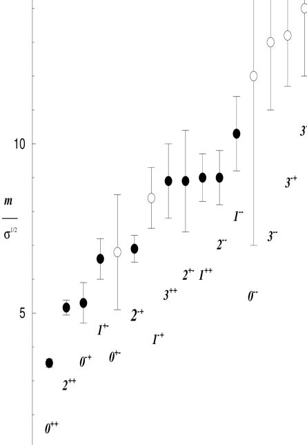
Figure 1.2: The mass of the glueball states with quantum numbers $J^{PC}$ from ref([6]). The scale is set by ${\sqrt{\sigma}}\approx 0.44$ GeV which yields the right hand scale in GeV. The solid points represent mass determinations whereas the open points are upper limits.

The predictions for the other $J^{PC}$ states are that they lie higher in mass and the present state of knowledge is summarised in fig. 2. Remember that the lattice results are strictly upper limits. For the $J^{PC}$ values not shown, these upper limits are too weak to be of use.

Since quark-antiquark mesons can only have certain $J^{PC}$ values, it is of special interest to look for glueballs with $J^{PC}$ values not allowed for such mesons: $0^{--}$, $0^{+-}$, $1^{-+}$, $2^{+-}$, etc. Such spin-exotic states, often called ‘oddballs’, would not mix directly with quark-antiquark mesons. This would make them a very clear experimental signal of the underlying glue dynamics. Various glueball models (bag models, flux tube models, QCD sum-rule inspired models,..) gave different predictions for the presence of such oddballs (eg. $1^{-+}$) at relatively low masses. The lattice mass spectra clarify these uncertainties but, unfortunately for experimentalists, do not indicate any low-lying oddball candidates. The lightest candidate is from the T${}_{2}^{+-}$ spin combination. Such a state could correspond to an $2^{+-}$ oddball. Another interpretation is also possible, however, namely that a non-exotic $3^{+-}$ state is responsible (this choice of interpretation can be resolved in principle by finding the degenerate 5 or 7 states of a $J=2$ or 3 meson). The overall conclusion at present is that there is no evidence for any oddballs of mass less than 3 GeV.

Returning briefly to the independence of the results on the volume of the lattice, in the early days of glueball mass determination, it was expected that a spatial size $L$ should satisfy $\hat{m}(0^{++})L>1$ and, hence, that values of $\hat{m}(0^{++})L$ of 1 to 4 would suffice. A careful lattice study[11] showed that $\hat{m}(0^{++})L>8$ was required to obtain rotational invariance and a result independent of $L$. The results collected in fig. 1 all satisfy this latter inequality so can be regarded as the infinite volume determination.

The small volume lattice results illustrate several points. One important feature is that closed loops of colour flux acting on the vacuum create glueballs but, if the loop encircles the periodic spatial boundary of length $L$, a torelon state can be created with energy given approximately by $KL$ where $K$ is the string tension. Thus at small $L$, the torelon state will be lighter than a glueball. In the quenched approximation, there is a $Z(N)$ symmetry of the lattice action which puts glueballs and torelons in different representations so they are unmixed. The fermion term in the action, however, breaks this symmetry so that for $N_{f}\not=0$, the lightest glueball will be very heavily contaminated by torelon-like contributions. In a semi-analytic study[8] this was explored and what is clear is that in a small volume the limit $N_{f}\to 0$ of full QCD is not equivalent to the quenched approximation with $N_{f}=0$.

Glueballs are defined in the quenched approximation and, hence, they do not decay into mesons since that would require quark-antiquark creation. It is, nevertheless, still possible to estimate the strength of the matrix element between a glueball and a pair of mesons within the quenched approximation. For the glueball to be a relatively narrow state, this matrix element must be small. A very preliminary attempt has been made to estimate the size of the coupling of the $0^{++}$ glueball to two pseudoscalar mesons[9]. A relatively small value of order 100 MeV is found. Further work needs to be done to investigate this in more detail, in particular to study the mixing between the glueball and $0^{++}$ mesons since this mixing may be an important factor in the decay process.

Another lattice study will become feasible soon. This is to study the glueball spectrum in full QCD vacua with sea quarks of mass $m_{\rm sea}$. For large $m_{\rm sea}$, the result is just the quenched result described above. For $m_{\rm sea}$ equal to the experimental light quark masses, the results should just reproduce the experimental meson spectrum — with the resultant uncertainty between glueball interpretations and other interpretations. The lattice enables these uncertainties to be resolved in principle: one obtains the spectrum for a range of values of $m_{\rm sea}$ between these limiting cases, so mapping glueball states at large $m_{\rm sea}$ to the experimental spectrum at light $m_{\rm sea}$. Studies conducted so far show no significant change of the glueball spectrum as dynamical quark effects are added — but the sea quark masses used are still rather large[12].

From the point of view of comparing quenched lattice results with models, a very useful system to study is the gluelump. This is the hydrogen atom of gluonic QCD: a system with one very heavy gluon which is treated as a static adjoint colour source and the surrounding gluonic field that makes a colour singlet hadron. In terms of experiment: this is the gluinoball formed from a gluino-gluon bound state which will be observable should massive gluinos exist and be sufficiently stable. The spectrum and spatial distribution of these states have been explored[13] for $SU(2)$ of colour. Because one colour source is fixed, the spatial size is easier to measure than for the glueballs themselves: the distributions were found to extend out to a radius of 0.5 fm. The ground state and first excited state were found to have quantum numbers consistent with being bound states of a magnetic gluon and an electric gluon respectively. For $SU(3)$ of colour the spectrum in the continuum limit has been determined[14] and the mass splitting between the two lightest of these states is found to be 350 MeV.

1.3 POTENTIALS BETWEEN QUARKS

A very straightforward quantity to determine from lattice simulation is the interquark potential in the limit of very heavy quarks (static limit). This potential is of direct physical interest because solving the Schrödinger equation in such a potential provides a good approximation to the $\Upsilon$ spectrum. It is also relevant to exploring both confinement and asymptotic freedom on a lattice.

The basic route to the static potential is to evaluate the average $W(\hat{R},\hat{T})$ in the vacuum samples of a rectangular closed loop of colour flux (a Wilson loop of size $\hat{R}\times\hat{T}$). This can be visualised as involving static sources $R$ apart with potential energy $V(R)$ for time $T$ so that $W\approx ce^{-V(R)T}$. More precisely, the lattice quantities $\hat{R}$ and $\hat{T}$ are related to the physical distances $R$ and $T$ by $\hat{R}=R/a$, etc where $a$ is the lattice spacing which is not known explicitly. Then it can be shown that the required static potential in lattice units is given by

$$\hat{V}(\hat{R})=\lim_{\hat{T}\to\infty}\log{W(\hat{R},\hat{T}-1)\over W(\hat{R},\hat{T})}$$ (1.10)

The limit of large $T$ is needed to separate the required potential from excited potentials. This limit can be made tractable in practice by using more complicated loops than the simple rectangular loop described above. The motivation for this is to generalise the straight paths of length $R$ at $t=0$ and $T$ by considering sums over paths that reflect more fully the colour flux between static quark and antiquark at separation $R$. Typically a smearing or fuzzing algorithm is used to create suitable wandering paths, then several such paths are combined in a variational approach to find the linear combination that best describes the ground state of the system: the potential $V(R)$.

Figure 1.3: The force between static quarks at separation $r$ as measured on lattices with different lattice spacing $a$ (with the $\beta$-values shown).

A summary of results[15, 16] for the potential at large $R$ is shown in figs 3, 4. The result that the force $dV/dR$ tends to a constant at large $R$ (and thus $V(R)$ continues to rise as $R$ increases) is a manifestation of the confinement of heavy quarks (in the quenched approximation). The force appears to approach a constant at large $R$. A simple parametrisation is traditional in this field:

$$V(R)=V_{0}-{e\over R}+KR$$ (1.11)

where $K$ (sometimes written $\sigma$) is the string tension. The term $e/R$ is referred to as the Coulombic part in analogy to the electromagnetic case. The equivalent relationship in terms of quantities defined on a lattice is

$$\hat{V}(\hat{R})=\hat{V}_{0}-{e\over\hat{R}}+\hat{K}\hat{R}$$ (1.12)

.

Figure 1.4: Potentials $V(R)$ between static quarks at separation $R$ for the ground state ($\Box$ and *) and for the $E_{u}$ symmetry which corresponds to the first excited state of the gluonic flux (octagons and diamonds). Results in lattice units ($a_{6.0}^{-1}=2.02$ GeV) from the quenched calculations of ref([16]) are shown by symbols corresponding to different lattice spacings. For the ground state potential the continuous curve is an interpolation of the lattice data while the dotted curve with enhanced Coulomb term fits the spectrum and yields the masses shown. The lightest hybrid level in the excited gluonic potential is also shown.

Since the string tension is given by the slope of $V(R)$ against $R$ as $R\to\infty$, this implies that some error will arise in determining $K$ coming from the extrapolation of lattice data at finite $R$. A practical resolution[17] is to define a value of $R$ where the potential takes a certain form. The convention is to use $r_{0}$ where

$$\left.{\hat{R}^{2}{d\hat{V}(\hat{R})\over d\hat{R}}}\right|_{\hat{r}_{0}}=1.65$$ (1.13)

Thus $\hat{r}_{0}$ can be determined by interpolation in $\hat{R}$ rather than extrapolation. In practice, this means that $\hat{r}_{0}$ is very accurately determined by lattice measurements and so is a useful quantity to use to set the scale since $\hat{r}_{0}=r_{0}/a$. With the simple parametrisation above, $r_{0}^{2}=(1.65-e)/K$ so $r_{0}$ is closely related to the string tension since $e\approx 0.25$. The string tension is usually taken from experiment as $\sqrt{K}=0.44$GeV where the value comes from $c\bar{c}$ and $b\bar{b}$ spectroscopy and from the light meson spectrum interpreted as excitations of a relativistic string. Similar analyses also imply that $r_{0}\approx 0.5$ fm. Here I use $r_{0}^{-1}=0.372$ GeV to be specific. Since I shall be describing quenched lattice results, the energy scale set from different physical quantities will not necessarily agree (since experiment has full QCD not the quenched vacuum) and so a systematic error of order 10% must be applied to any such choice of scale. This was discussed when taking glueball mass values from quenched lattice calculations.

The lattice potential $V(R)$ can be used to determine the spectrum of $b\bar{b}$ mesons by solving Schrödinger’s equation since the motion is reasonably approximated as non-relativistic. The lattice result is similar to the experimental $\Upsilon$ spectrum. The main difference is that the Coulombic part ($e$) is effectively too small (0.28 rather than 0.4). This produces[16] a ratio of mass differences $(1P-1S)/(2S-1S)$ of 0.71 to be compared with the experimental ratio of 0.78. This difference is understandable as a consequence of the Coulombic force at short distances which would be increased by $33/(33-2N_{f})$ in perturbation theory in full QCD compared to quenched QCD. I will return to discuss this in the context of lattice dynamical fermion calculations[18].

1.3.1 Running coupling constant

At small $R$, the static potential can be used, in principle, to study the running coupling constant. Small $R$ corresponds to large momentum and the coupling should decrease at small $R$. Thus the Coulombic coefficient $e$ introduced above should actually decrease logarithmically as $R$ decreases. Perturbation theory can be used to determine this behaviour of the potential at small $R$.

In the continuum the potential between static quarks is known perturbatively to two loops in terms of the scale $\Lambda_{{\rm\overline{MS\kern-0.98pt}\kern 0.98pt}}$. For $SU(3)$ colour, the continuum force is given for $N_{f}=0$ by[19]

$${dV\over dR}={4\over 3}{\alpha(R)\over R^{2}}$$ (1.14)

with the effective coupling $\alpha(R)$ given by

$${1\over 4\pi[b_{0}\log(R\Lambda_{F})^{-2}+(b_{1}/b_{0})\log\log(R\Lambda_{F})^{-2}]}$$ (1.15)

where $b_{0}=11/16\pi^{2}$ and $b_{1}=102\ b_{0}^{2}/121$ are the usual coefficients in the perturbative expression for the $\beta$-function, neglecting quark loops in the vacuum. Here $\Lambda_{F}=1.048\Lambda_{{\rm\overline{MS\kern-0.98pt}\kern 0.98pt}}$.

This perturbative result can be used to define a running coupling constant non-perturbatively. Thus a coupling in the ‘force’ scheme can be defined by

$$\alpha_{F}(R)\equiv{3\over 4}R^{2}{dV\over dR}$$ (1.16)

Different non-perturbative definitions of $\alpha$ can be related using perturbation theory, for example the one loop comparison of $\alpha_{F}$ and $\alpha_{{\rm\overline{MS\kern-0.98pt}\kern 0.98pt}}$ gives the relationship between the respective $\Lambda$ values quoted above.

On a lattice the force can be estimated by a finite difference and one can extract the running coupling constant by using[20]

$$\alpha_{F}({\hat{R}_{1}+\hat{R}_{2}\over 2})={3\over 4}\hat{R}_{1}\hat{R}_{2}{\hat{V}(\hat{R}_{1})-\hat{V}(\hat{R}_{2})\over\hat{R}_{1}-\hat{R}_{2}}$$ (1.17)

where the error in using a finite difference is negligible in practice.

This is plotted in fig. 5 versus $RK^{1/2}$: this combination is dimensionless and so can be determined from lattice results since $RK^{1/2}=\hat{R}\hat{K}^{1/2}$, where $\hat{K}$ is taken from the fit to $\hat{V}(\hat{R})$. The interpretation of $\alpha_{F}$ as defined above as an effective running coupling constant is only justified at small $R$ where the perturbative expression dominates. Also shown are the two-loop perturbative results for $\alpha(R)$ for different values of $\Lambda_{F}$.

Figure 1.5: The effective running coupling constant $\alpha_{F}(R)$ obtained from the force between static quarks at separation $R$ from ref([21]). The scale is set by the string tension $K$. Data are at $\beta=6.5$ (diamonds) and at $\beta=6.2$ (triangles). The dotted error bars represent an estimate of the systematic error due to lattice artefact corrections. The curves are the two-loop perturbative expression with $a(6.5)\Lambda_{F}=0.060$ (dotted) and 0.070 (continuous).

Fig. 5 clearly shows a running coupling constant. Moreover the result is consistent with the expected perturbative dependence on $R$ at small $R$. There are systematic errors, however. At larger $R$, the perturbative two-loop expression will not be an accurate estimate of the measured potentials, while at smaller $R$, the lattice artefact corrections (which arise because $R/a\approx 1$) are relatively big. Setting the scale using $\sqrt{K}=0.44$ GeV implies $1/a(\beta=6.5)=4.13$ GeV, so $R<4a(6.5)$ corresponds to values of $1/R>1$ GeV. This $R$-region is expected to be adequately described by perturbation theory. Other methods to extract a running coupling from lattice results have been used and some have smaller systematic errors. For a comparison see ref([22]).

This determination from the interquark force of the coupling $\alpha$ allows us to compare the result with the bare lattice coupling determined from $\beta=6/g^{2}$. At $\beta=6.5$, $\alpha_{\rm bare}=g^{2}/4\pi=0.073$. The values of $\alpha$ shown in fig. 5 are much larger. The effective coupling constant is thus almost twice the bare coupling. This is quite acceptable in a renormalisable field theory. The message is that the bare coupling should be disregarded — it is not a good expansion parameter. The measured $\alpha_{F}$, however, proves to be a reasonable expansion parameter in the sense that the first few terms of the perturbation series converge. This successful calibration of perturbation theory on a lattice is important in practice. For instance, when matrix elements are measured on a lattice they have finite correction factors (usually called Z) to relate them to continuum matrix elements. These Z factors are evaluated perturbatively — so an accurate continuum prediction needs trustworthy perturbative calculations.

1.3.2 Excited gluonic modes

The situation of a static quark and antiquark is a very clear case in which to discuss hybrid mesons which have excited gluonic contributions. A discussion of the colour representation of the quark and antiquark is not useful since they are at different space positions and the combined colour is not gauge invariant. A better criterion is to focus on the spatial symmetry of the gluonic flux. As well as the symmetric ground state of the colour flux between two static quarks, there will be excited states with different symmetries. These were studied on a lattice[23] and the conclusion was that the $E_{u}$ symmetry (corresponding to flux states from an operator which is the difference of U-shaped paths from quark to antiquark of the form $\,\sqcap-\sqcup$) was the lowest lying gluonic excitation. Results for this potential are shown in fig. 4.

This gluonic excitation corresponds to a component of angular momentum of one unit along the quark antiquark axis. Then one can solve for the spectrum of hybrid mesons using the Schrödinger equation in the adiabatic approximation. The spatial wave function necessarily has non zero angular momentum and corresponds to $L^{PC}=1^{+-}$ and $1^{-+}$. Combining with the quark and antiquark spins then yields[23] a set of 8 degenerate hybrid states with $J^{PC}=1^{--},\ 0^{-+},\ 1^{-+},\ 2^{-+}$ and $1^{++},\ 0^{+-},\ 1^{+-},\ 2^{+-}$ respectively. These contain the spin-exotic states with $J^{PC}=1^{-+},\ 0^{+-}$ and $2^{+-}$ which will be of special interest.

Since the lattice calculation of the ground state and hybrid masses allows a direct prediction for their difference, the result for this 8-fold degenerate hybrid level is illustrated in fig. 4 and corresponds[16] to masses of 10.81(25) GeV for $b\bar{b}$ and 4.19(15) GeV for $c\bar{c}$. Here the errors take into account the uncertainty in setting the ground state mass using the quenched potential as discussed above. Recently a different lattice technique[24] has been used to explore the excited gluonic levels in the quenched approximation. The results above are confirmed and preliminary values quoted for the lightest hybrid mesons are 10.83 and 4.25 GeV respectively for $b\bar{b}$ and $c\bar{c}$ with no error estimates given.

The quenched lattice results show that the lightest hybrid mesons lie above the open $B\bar{B}$ threshold and are likely to be relatively wide resonances. This could also be checked by comparing with quenched masses for the $B$ meson itself[26], but at present there are quite large uncertainties on that mass determination. The very flat potential implies a very extended wavefunction: this has the implication that the wavefunction at the origin will be small, so hybrid vector states will be weakly produced from $e^{+}e^{-}$.

It would be useful to explore the splitting among the 8 degenerate $J^{PC}$ values obtained. This could come from different excitation energies in the $L^{PC}=1^{+-}$ (magnetic) and $1^{-+}$ (pseudo-electric) gluonic excitations, spin-orbit terms, as well as mixing between hybrid states and $Q\bar{Q}$ mesons with non-exotic spin. One way to study this on a lattice is to use the NRQCD formulation which describes non-static heavy quarks which propagate non-relativistically. Preliminary results for hybrid excitations from several groups[25] give at present similar results to those with the static approximation as described above, but future results may be more precise and able to measure splittings among different states.

As well as comparing excited gluonic states from the lattice with experimental spectra for $\bar{b}b$ systems, it is also worthwhile to compare with phenomenological models. One such model is the hadronic string. This has the simple prediction that gluonic excitations are at multiples of $\pi/R$ in energy higher at large $R$. A detailed comparison[16] for SU(2) of colour shows qualitative agreement of the lattice excited potentials with the string model provided an appropriate expression is used for excited level $j$:

$$V_{j}(R)=(K^{2}R^{2}-{\pi K\over 6}+2\pi jK)^{1\over 2}.$$ (1.18)

This expression also shows that even the ground state string mode ($j=0$) will have a contribution from a string fluctuation, namely[27] $V(R)\approx KR-\pi/(12R)$ as $R\to\infty$. In practice this $1/R$ string fluctuation term is very hard to disentangle from the Coulomb term $e/R$. One way to get round this in lattice studies is to consider a hadronic string that encircles the periodic spatial boundaries of length $L$. Then there are no sources and hence no Coulomb component. The appropriate string fluctuation term in the energy of this state, called the torelon, is then given by $E(L)=KL+\pi/(3L)$ as $L\to\infty$. Lattice studies[28] have confirmed the presence of this string fluctuation term with the correct coefficient as given to a precision of 3%. This is impressive evidence that the hadronic string is a good model of the energy of the colour flux tube at large distances.

1.3.3 Confinement

The simplest manifestation of confinement is that the potential $V(R)$ between static colour sources in the fundamental representation continues to rise with increasing $R$ in quenched QCD. This raises the question of the nature of the colour fields between the sources. Lattice studies have been undertaken[29, 30] to probe the energy momentum tensor of these colour fields. The probe used is a plaquette so the momentum scale of the probe increases as $a\to 0$. Lattice sum rules [30] can be used to normalise these distributions and relate them to the $\beta$-function. For separation $R>0.7$ fm, a string-like spatial distribution is found where the transverse width of the flux tube increases slowly at most with increasing $R$. For these $R$ values, the averages of the squared components of the colour fields (these are gauge invariant quantities) are found to be roughly equal (i.e. $E^{2}_{i}\approx B^{2}_{j}$, for all $i,\ j=1,\ 2,\ 3$). This implies that the energy density is much smaller than the action density. As well as components of the energy-momentum tensor which are gauge invariant, it is possible to study the colour field tensors directly by choosing a suitable gauge[31].

Another detail concerning the confining force is its spin dependence. A lattice study of the spin-spin and spin-orbit potentials between static quarks allows this to be explored. The basic conclusion[32] is that the only long-range force is a spin-orbit force of the type usually called scalar. More recent studies[33] confirm this. This lattice result is confirmed by phenomenological studies of the observed splitting between P-wave $\bar{b}b$ and $\bar{c}c$ states.

Another route to explore confinement is to measure on a lattice the potential energy between two static sources in the adjoint representation of the colour group. At large $R$ the adjoint potential $V_{A}(R)$ must become a constant because each adjoint colour source can be screened by a gluonic field. Indeed at large $R$, $V_{A}\to 2m_{\rm gluelump}$ where the gluelump is the ground state hadron with a gluon field around a static adjoint: the gluinoball. Of interest to model builders is the adjoint potential at smaller $R$ values. The most precise data are for $SU(2)$ of colour[34] and they do show a region of linear rise, although with a slope less steep than that given by the Casimir ratio (namely ${8\over 3}V(R)$ where $V(R)$ is the fundamental colour source potential discussed previously). Attempts have also been made[35] to explore the colour field distributions in this case.

1.4 LIGHT QUARKS — HYBRIDS

Unlike very heavy quarks, light quark propagation in the gluonic vacuum sample is very computationally intensive — involving inversion of huge ($10^{7}\times 10^{7}$) sparse matrices. Current computer power is sufficient to study light quark physics thoroughly in the quenched approximation. The state of the art[36] is the Japanese CPPACS Collaboration who are able to study a range of large lattices (up to about $64^{4}$) with a range of light quark masses. Qualitatively the meson and baryon spectrum of states made of light and strange quarks is reproduced with discrepancies of order 10% in the quenched approximation.

Figure 1.6: The masses in lattice units (with $a_{6.0}^{-1}\approx 2$ GeV) of states of $J^{PC}$ built from hybrid operators with strange quarks, spin-exotic (*) and non-exotic ($\Box$). The dot-dashed lines are the mass values found for $s\bar{s}$ operators. Results from ref([37]).

Here I will focus on hybrid mesons made from light quarks. In the quenched approximation, there will be no mixing involving spin-exotic hybrid mesons and so these are of special interest. The first study of this area was by the UKQCD Collaboration[37] who used operators motivated by the $Q\bar{Q}$ studies referred to above. Using non-local operators, they studied all 8 $J^{PC}$ values coming from $L^{PC}=1^{+-}$ and $1^{-+}$ excitations. The resulting mass spectrum is shown in fig. 6 where the $J^{PC}=1^{-+}$ state is seen to be the lightest spin-exotic state with a statistical significance of 1 standard deviation. The statistical error on the mass of this lightest spin-exotic meson is 7% but to take account of systematic errors from the lattice determination a mass of 2000(200) MeV is quoted for the $s\bar{s}$ meson. Although not directly measured, the corresponding light quark meson would be expected to be around 120 MeV lighter. In view of the small statistical error, it seems unlikely that the $1^{-+}$ meson in the quenched approximation could lie as light as 1.4 GeV where there are experimental indications for such a state[38]. Beyond the quenched approximation, there will be mixing between such a hybrid meson and $q\bar{q}q\bar{q}$ states such as $\eta\pi$ and this may be significant.

One feature clearly seen in fig. 6 is that non spin-exotic mesons created by hybrid meson operators have masses which are very similar to those found when the states are created by $q\bar{q}$ operators. This suggests that there is quite strong coupling between hybrid and $q\bar{q}$ mesons even in the quenched approximation. This would imply that the $\pi(1800)$ is unlikely to be a pure hybrid, for example.

A second lattice group has also evaluated hybrid meson spectra from light quarks. They obtain[39] masses with statistical and various systematic errors for the $1^{-+}$ state of 1970(90)(300) MeV, 2170(80)(100)(100) MeV and 4390(80)(200) MeV for $n\bar{n}$, $s\bar{s}$ and $c\bar{c}$ quarks respectively. For the $0^{+-}$ spin-exotic they have a noisier signal but evidence that it is heavier. They also explore mixing matrix elements between spin-exotic hybrid states and 4 quark operators.

1.5 FULL QCD

So far I have discussed the glueball spectrum, interquark potentials and $\alpha_{S}$ in the quenched approximation. This corresponds to treating the sea quarks as of infinite mass (so they don’t contribute to the vacuum). To make direct comparison with experiment, it is necessary to estimate the corrections from these dynamical quark loops in the vacuum.

The strategy is to use a finite sea-quark mass but still a value larger than the empirical light quark mass. The reason is computational: the algorithms become very inefficient as the sea-quark mass is reduced. The target is to study the effects as the sea-quark mass is reduced and then extrapolate to the physical value. The present situation, in broad terms, is that there is no significant change as the sea-quark mass is reduced. This could be because there are no corrections to the quenched approximation. Alternatively, the corrections may only turn on at a much lower quark mass than has been explored so far.

Let us try to make this argument a little more quantitative. For heavy sea-quarks of mass $m$, their contribution will be approximately proportional to $e^{-2m/E}$ where $E$ is a typical hadronic energy scale (a few hundred MeV). Thus the quark loop contributions will be negligible for $m>>E$, which corresponds to the quenched approximation. As $m\approx E$, the effects will turn on in a non-linear way.

The computational overhead of full QCD on a lattice is so large because the quark loops effectively introduce a long range interaction. The quark interaction in the action is quadratic and so can be integrated out analytically — see eq(5). This leaves an effective action for the gluonic fields which couples together the fields at all sites. This implies that, in a Monte Carlo method, a change in gluon field at one site involves the evaluation of the interaction with all other sites. In practice, one makes small changes at all sites in parallel, but this still amounts to inverting a large sparse matrix for each update. This is computationally slow.

As the sea-quark mass becomes small, one would expect to need a larger lattice size to hold the quarks. For heavy quarks, the effective range of the quark loops in the vacuum will be of order $1/m$. Thus the quenched approximation corresponds to $m\to\infty$ and a local interaction. For light quarks of a few MeV mass, the range will not be $1/m$, because quarks are confined. The lattice studies that have been made suggest that spatial sizes of order twice those adequate for the quenched approximation are needed for full QCD. This also implies considerable computational commitment.

A popular indication of how close a full QCD study is to experiment is to ask whether the $\rho$ meson can decay to two pions. Since the decay is P-wave, it needs non-zero momentum. On a lattice spatial momentum is quantised in units of $2\pi/L$. Thus $m_{V}>2({m_{P}}^{2}+4\pi^{2}/L^{2})^{1/2}$ for the decay channel to be allowed energetically. At present this criterion is rarely satisfied in quenched studies, let alone in the more computationally demanding case of full QCD.

The conclusion of current full QCD lattice calculations is that the expected sea-quark effects are not yet fully present. The main effect observed in full QCD calculations is that the lattice parameter $\beta$ which multiplies the gluonic interaction term in the action is shifted. Apart from this renormalisation of $\beta$, there is little sign of any other statistically significant non-perturbative effect.

Consider the changes to be expected for the inter-quark potential when the full QCD vacuum is used:

• At small separation $R$, the quark loops will increase the size of the effective coupling $\alpha$ compared to the pure gluonic case. This effect can be estimated in perturbation theory and the change at lowest order will be from 1/33 to 1/(33-$2N_{f}$).

• At large separation $R$, the potential energy will saturate at a value corresponding to two ‘heavy-quark mesons’. In other words, the flux tube between the static quarks will break by the creation of a $q\bar{q}$ pair from the vacuum.

Current lattice simulation[18] shows some evidence for the former effect but no statistically significant signal for the latter.

1.6 OUTLOOK

Lattice QCD is good for asking ‘what’ not ‘why’. Lattice results for masses and matrix elements are obtained from first principles without approximations (except in many cases the quenched approximation is still needed to keep the computational resource manageable). No model is used but no understanding of the underlying physics is obtained. By varying the quark masses, boundary conditions etc, it is possible to explore a much wider range of circumstances than is available directly from experiment. This is a very valuable tool for validating models and learning ‘why’.

Lattice techniques can extract reliable continuum properties from QCD. At present, the computational power available combined with the best algorithms suffices to give accurate results for many quantities in the quenched approximation. The future is to establish accurate values for more subtle quantities in the quenched approximation (eg. weak matrix elements of strange particles) and to establish the corrections to the quenched approximation by full QCD calculations.

I hope that soon we reach the stage where an experimentalist saying ‘as calculated in QCD’ is assumed to be speaking of non-perturbative lattice calculations rather than perturbative estimates only.

Bibliography

- [1] H. Rothe, Lattice Gauge Theories, World Scientific, 1992; I. Montvay and G. Münster, Quantum Fields on a Lattice, CUP, 1994.
- [2] K. G. Wilson, Phys. Rev. D10:2445 (1974).
- [3] G. P. Lepage and P. B. Mackenzie, Phys. Rev. D48:2250 (1993).
- [4] P. De Forcrand, et al., Phys. Lett. B152:107 (1985).
- [5] C. Michael and M. Teper, Nucl. Phys. B314:347 (1989).
- [6] UKQCD collaboration, G. Bali, K. Schilling, A. Hulsebos, A. C. Irving, C. Michael and P. Stephenson, Phys. Lett. B309:378 (1993).
- [7] H. Chen, J. Sexton, A. Vaccarino, and D. Weingarten, Nucl. Phys. B (Proc. Suppl.) 34:357 (1994).
- [8] J. Kripfganz and C. Michael, Nucl. Phys. B314:25 (1989).
- [9] J. Sexton, A. Vaccarino, and D. Weingarten, Phys. Rev. Lett. 75:4563 (1995).
- [10] C. Morningstar, and M. Peardon, hep-lat/9704011.
- [11] C. Michael, G. A. Tickle and M. Teper, Phys. Lett. B207:313 (1988).
- [12] SESAM Collaboration, G. Bali et al., Nucl. Phys. B (Proc. Suppl.) 53:239 (1997).
- [13] I. Jorysz and C. Michael, Nucl. Phys. B302:448 (1988).
- [14] M. Foster and C. Michael, Nucl. Phys. B (Proc. Suppl.) (LAT97 in press), hep-lat/9709051.
- [15] G.S. Bali and K. Schilling, Phys. Rev. D47:661 (1993); H. Wittig (UKQCD collaboration), Nucl. Phys. B (Proc. Suppl) 42:288 (1995).
- [16] S. Perantonis and C. Michael, Nucl. Phys. B347:854 (1990).
- [17] R. Sommer, Nucl. Phys. B411:839 (1994).
- [18] SESAM Collaboration, U. Glässner, et al., Phys. Lett. B383:98 (1966); S. Güsken , Nucl. Phys. B (Proc. Suppl.) (LAT97 in press).
- [19] A. Billoire, Phys. Lett. B104:472 (1981).
- [20] C. Michael, Phys. Lett. B283:103 (1992)
- [21] UKQCD collaboration, A. Hulsebos et al., Phys. Lett. B294:385 (1992).
- [22] C. Michael, Nucl. Phys. B (Proc. Suppl.) 42:147 (1995).
- [23] L. Griffiths, C. Michael, and P. Rakow, Phys. Lett. B129:351 (1983).
- [24] K. Juge, J. Kuti and C. Morningstar, Nucl. Phys. B (Proc. Suppl.) (in press), heplat/9709131.
- [25] A. Alikhan, Nucl. Phys. B (Proc. Suppl.) (LAT97 in press).
- [26] R. Sommer, Phys. Rep. 275:1 (1996).
- [27] M. Lüscher, Nucl. Phys. B180[FS2]:317 (1981).
- [28] C. Michael and P. Stephenson, Phys. Rev. D50:4634 (1994).
- [29] G. Bali, K. Schilling and C. Schlichter, Phys. Rev. D51:5165 (1995).
- [30] A. M. Green, C. Michael and P. Spencer, Phys. Rev. D55:1216 (1997).
- [31] A. Di Giacomo et al., Nucl. Phys. B347:441 (1990).
- [32] C. Michael, Phys. Rev. Lett. 56:1219 (1986).
- [33] G. Bali, A. Wachter and K. Schilling, Phys. Rev. D55:5309 (1997); D56:2566 (1997).
- [34] C. Michael, Nucl. Phys. B (Proc. Suppl.) 26:417 (1992).
- [35] H. Trottier, Nucl. Phys. B. (Proc. Suppl.) 47:286 (1996).
- [36] T. Yoshie, Nucl. Phys. B (Proc. Suppl.) (LAT97 in press).
- [37] UKQCD Collaboration, P. Lacock, C. Michael, P. Boyle, and P. Rowland, Phys. Rev. D54:6997 (1996); Phys. Lett. B401:308 (1997); Nucl. Phys. B (Proc. Suppl.) (LAT97 in press), hep-lat/9708013.
- [38] A. Ostrovidov, Proc. Hadron97, BNL.
- [39] C. Bernard, et al., Nucl. Phys. B (Proc. Suppl.) 53:228 (1996); hep-lat/9707008.