Next–to–Leading Order QCD corrections

for the $B^{0}\overline{B^{0}}$-mixing with an extended Higgs sector

J. Urban, F. Krauss, U. Jentschura, G. Soff

Institut f$\ddot{\rm u}$r Theoretische Physik

Technische Universit$\ddot{\rm a}$t Dresden

Mommsenstr.13, D-01062 Dresden, Germany

Abstract

We present a calculation of the $B^{0}\overline{B^{0}}$–mixing including Next–to–Leading Order (NLO) QCD corrections within the Two Higgs Doublet Model (2HDM). The QCD corrections at NLO are contained in the factor denoted by $\eta_{2}$ which modifies the result obtained at the lowest order of perturbation theory. In the Standard Model case, we confirm the results for $\eta_{2}$ obtained by Buras, Jamin and Weisz [1]. The factor $\eta_{2}$ is gauge and renormalization prescription invariant and it does not depend on the infrared behaviour of the theory, which constitutes an important test of the calculations. The NLO–calculations within the 2HDM enhance the LO–result up to $18\,\%$, which affects the correlation between $M_{H}$ and $V_{td}$.

PACS-numbers: 12.15.Ff; 12.60.Fr; 14.80.Cp; 12.38.Bx
Key–words: Mixing; Oscillations; 2HDM; CP-violation; CKM-matrix

1 Introduction

The $B$-meson plays an important role in present day physics. $B^{0}\overline{B^{0}}$–mixing as well as $B$-meson decays can be used to determine the CKM–elements and to investigate $CP$-violation within the Standard Model (SM). Two large experiments, namely the BABAR-Collaboration at SLAC [2] and the Belle Collaboration at KEK [3], will start taking data in the near future. The major subject of research in those experiments is the determination of the CKM–matrix elements. This may also provide first hints on physics beyond the Standard Model.

In general terms $B^{0}\overline{B^{0}}$–mixing is a Flavour Changing Neutral Current (FCNC) process generated through weak interactions. In the SM, the process is generated at the lowest order of perturbation theory via the box diagrams displayed in Fig. 2. Due to the large difference in the masses of heavy particles in the box ($W^{\pm}$, $H^{\pm}$ and $t$–quarks) and much lighter external particles ($b$ and $d$–quarks), it is possible to disentangle long and short distance effects. This can be accomplished within an effective theory. The proper separation of short and long distance QCD-effects at Next–to–Leading Order was first presented for the SM in  [1]. We are utilizing here the same framework of renormalization group improved perturbation theory.

Our purpose is to include two Higgs–boson doublets as an extended Higgs–boson sector. Such models are usually called Two Higgs Doublet Models (2HDM)  [4, 5]. Two particular models which are usually considered (so–called Model I and Model II) differ in the couplings of the charged Higgs–bosons to fermions (see for example [4]):

$${\cal L}_{H\,ud}^{I} = \frac{g_{W}V_{ud}}{\sqrt{2}m_{W}}\left[m_{u}\cot(\beta)P_{L}-m_{d}\cot(\beta)P_{R}\right]\;,$$ (1)

$${\cal L}_{H\,ud}^{II} = \frac{g_{W}V_{ud}}{\sqrt{2}m_{W}}\left[m_{u}\cot(\beta)P_{L}+m_{d}\tan(\beta)P_{R}\right]\;.$$ (2)

Here $g_{W}$ is the weak coupling constant, $m_{W}$ is the $W$–mass, and the projectors $P_{L,R}$ are defined by

$$P_{L,R}=\frac{1\mp\gamma_{5}}{2}\;.$$ (3)

The subscripts $u$ and $d$ denote up– and down–type quarks, respectively.

As we neglect all quark masses except $m_{t}$, both models are identical in our case. Thus our calculations are valid for all values of $\tan\beta$ for the Model I, but only for $\tan\beta<<m_{t}/m_{b}$ in the Model II. Looking at the Feynman rules for the Higgs–quark–quark coupling, it is easy to verify that in Model II, the term proportional to $m_{b}$ becomes important for large values of $\tan\beta$. Due to the projectors in the vertex, we would end up with different operators for the $\tan\beta$ and $\cot\beta$ parts. However, it should be stressed here that Model II is more interesting, because this is the choice favoured by the Minimal Supersymmetric Standard Model [4, 6]. Large values of $\tan\beta$ will be considered in a future publication.

We continue our discussion with a short review of the Leading Order (LO) calculations. The basic idea is rather simple. First, one has to calculate the box diagrams in Fig.2. They can be evaluated in the Feynman–’t Hooft gauge for the $W$–boson. This leaves us with a physical $W$–boson and a would-be Goldstone boson (unphysical scalar Higgs boson) of the same mass and with couplings proportional to the quark masses. As all quark masses except the top–quark mass are equal to zero to a good approximation, $t$ is the only active flavour in boxes containing Higgs particles or unphysical scalars. In the remaining box diagrams, the effects of u- and c- quarks are taken into account by the GIM mechanism. Evaluating the box diagrams in this framework leads to the well known Inami–Lim functions  [7]–[10].

The scaling behaviour from the matching scale $\mu_{0}=m_{W}$ of the full and effective theory down to a lower scale is then determined by the one–loop QCD correction to the effective vertex generated by the previous procedure of integrating out the internal heavy degrees of freedom. The renormalization group equation gives us the factor $\overline{\eta}_{LO}$ describing the effect of scaling  [11].

The effective Hamiltonian for $B^{0}\overline{B^{0}}$–mixing at LO reads

$$H_{\rm{eff}}\;=\frac{1}{4}\,{G^{2}_{F}\over\pi^{2}}\;m_{W}^{2}\;{(V_{td}V^{\ast}_{tb})}^{2}\;\overline{\eta}_{LO}\;S(x_{W},x_{H})\;\hat{\cal O}_{LL}\;,$$ (4)

where

$$\hat{\cal O}_{LL}=\biggl{[}\;\bar{d}\;\gamma_{\mu}\;P_{L}\;b\;\biggr{]}\;\biggl{[}\;\bar{d}\;\gamma^{\mu}\;P_{L}\;b\;\biggr{]}\;$$ (5)

and

$$S(x_{W},x_{H})\;=\;S_{WW}(x_{W})+2\,S_{WH}(x_{W},x_{H})+S_{HH}(x_{H})\;.$$ (6)

The LO Inami–Lim functions $S_{WW}(x_{W})$, $S_{WH}(x_{W},x_{H})$ and $S_{HH}(x_{H})$ can be found in Appendix A. The arguments of the Inami–Lim–functions will be denoted $x_{W,H}=m_{t}^{2}/m_{W,H}^{2}$.

The factor $\overline{\eta}_{LO}$ is determined by the $\beta$–function [12] and the anomalous dimension $\gamma$ to be obtained by evaluating the diagrams of Fig. 2. It reads

$$\overline{\eta}_{LO}\;=\;\biggl{[}\;{{\alpha_{S}(m_{W})}\over{\alpha_{S}(m_{B})}}\;\biggr{]}^{\gamma^{(0)}/(2\beta_{0})}\;=\;\biggl{[}\;{{\alpha_{S}(m_{W})}\over{\alpha_{S}(m_{B})}}\;\biggr{]}^{6/23}\approx 0.85\;.$$ (7)

For later convenience we define $\eta_{LO}=\alpha_{S}(m_{W})^{(6/23)}$.

To evaluate the matrix element of $H_{\rm{eff}}$ we have to employ

$$\langle\bar{B}^{0}|\hat{\cal O}_{LL}|B^{0}\rangle\;=\;{2\over 3}\;B_{B}\;(\mu)\;f^{2}_{B}\;m^{2}_{B}\;,$$ (8)

where $f_{B}$ is the $B$–meson decay constant and $B_{B}(\mu)$ parameterizes deviations from the vacuum insertion approximation.

2 Explicit QCD-Corrections

The perturbative result for ${\cal O}(\alpha_{S})$ corrections in 2HDM will be presented in this section. The results can be obtained by evaluation of the diagrams of Figs. 3 and 4. We performed our calculation in an arbitrary covariant $\xi$-gauge for the gluon and we employed the Feynman–’t Hooft gauge for the $W$–boson.

As one easily notices, the diagrams a, b and f - i have the ” octet”–structure $\hat{T}_{a}\otimes\hat{T}^{a}$, whereas the diagrams c - e and j have ” singlet”–structure $\hat{\bf 1}\otimes\hat{\bf 1}$ in colour space. The double penguin diagram k contributes to the considered process at the order of ${\cal O}(1/m_{W}^{4})$ which is negligible for our purpose.

Diagrams containing vertex– and self–energy corrections (diagrams c, d and e) lead to UV-divergent integrals and hence they have to be regularized and renormalized. We are using dimensional regularization with anticommuting $\gamma_{5}$. This corresponds to the NDR–scheme (“naive” dimensional regularization scheme) [13, 14]. We performed the necessary renormalization in the $\overline{MS}$–scheme [13, 15]. All other diagrams are UV–finite. Furthermore, one notices that the diagrams g - j contain infrared divergences. To deal with them we keep the external quark masses whenever necessary. As we will see, the external quark masses do not affect the final result for the Wilson–coefficient. This justifies the method we have chosen.

We could also treat the infrared divergences with the method of dimensional regularization  [16], but our intention was to verify the results provided by Buras and collaborators in  [1] and to extend these calculations to the 2HDM.

The ${\cal O}(\alpha_{S})$-corrections to the Hamiltonian (4) have the following structure

$$\langle\Delta H_{\rm{eff}}\rangle\;=\frac{1}{4}\,{G^{2}_{F}\over\pi^{2}}\;m_{W}^{2}\;{\alpha_{S}\over 4\pi}\;(V_{td}V^{\ast}_{tb})^{2}\;U(x_{W},x_{H})\;,$$ (9)

where

$$U(x_{W},x_{H})=\sum_{k}\;\biggl{(}C_{F}\,\hat{\bf 1}\otimes\hat{\bf 1}\,\phi^{(1)}_{k}(x_{W},x_{H})+\hat{T}_{a}\otimes\hat{T}^{a}\,\phi^{(8)}_{k}(x_{W},x_{H})\biggr{)}\langle\hat{\cal O}_{k}\rangle$$ (10)

with $k\in\{LL,1,2,3\}$. $C_{F}$ is the colour-factor defined by $C_{F}=(N_{c}^{2}-1)/(2N_{c})$ and $N_{c}$ is the number of colours.

The operators $\hat{\cal O}_{i}$ read

$$\hat{\cal O}_{LL} = \left[\bar{d}\;\gamma_{\mu}\,P_{L}\;b\right]\left[\bar{d}\;\gamma^{\mu}\,P_{L}\;b\right]\;,$$ (11)

$$\hat{\cal O}_{1} = \left[\bar{d}\;P_{L}\;b\right]\left[\bar{d}\;P_{L}\;b\right]-{1\over 4}\left[\bar{d}\;\sigma_{\mu\nu}\,P_{L}\;b\right]\left[\bar{d}\;\sigma^{\mu\nu}\,P_{L}\;b\right]+(P_{L}\longrightarrow P_{R})\;,\;$$ (12)

$$\hat{\cal O}_{2} = \left[\bar{d}\;P_{L}\;b\right]\left[\bar{d}\;P_{R}\;b\right]+\left[\bar{d}\;P_{R}\;b\right]\left[\bar{d}\;P_{L}\;b\right]\;,$$ (13)

$$\hat{\cal O}_{3} = \left[\bar{d}\;\gamma_{\mu}\,P_{L}\;b\right]\left[\bar{d}\;\gamma^{\mu}\,P_{R}\;b\right]+(P_{L}\longleftrightarrow P_{R})\;.$$ (14)

The operator $\hat{\cal O}_{1}$ steems from diagrams g and h in Fig. 4, whereas the operators $\hat{\cal O}_{2}$ and $\hat{\cal O}_{3}$ follow from diagrams i and j, respectively. Since the relevant operator $\hat{\cal O}_{LL}$ is self–conjugate under Fierz–transformations, we will use

$$\hat{T}_{a}\otimes\hat{T}^{a}=C_{A}\hat{\bf 1}\otimes\hat{\bf 1}=\frac{1}{2}\left(1-\frac{1}{N_{c}}\right)\hat{\bf 1}\otimes\hat{\bf 1}\;$$ (15)

to retain only one operator. Nevertheless, to keep the calculations transparent, we will abandon the distinction between octet and singlet at the very end only.

The coefficient functions $\phi$ in equation (10) can be decomposed as

$$\noindent\phi^{(i)}_{j}=\chi^{(i,SM)}_{j}(x_{W})+\chi^{(i,H)}_{j}(x_{W},x_{H})\;.$$ (16)

The functions $\chi^{(i,SM)}_{j}(x_{W})$ were already given in ref.  [1]. We have recalculated them and we confirm these Standard Model results.

$$\noindent\chi^{(1,SM)}_{LL}(x_{W}) = L^{(1,SM)}(x_{W})+\left[2\,\xi\ +2\,\xi\,g_{IR}\,+2\,\xi\,\ln(x_{\mu_{0}})+6\,\ln(x_{\mu_{0}})\;x_{W}\,{\partial\over\partial x_{W}}\right]S_{WW}(x_{W})\;,$$

$$\chi^{(8,SM)}_{LL}(x_{W}) = L^{(8,SM)}(x_{W})+\left[2\,\xi\,+(3+\xi)\ln(x_{b}\,x_{d})\,+2\,\xi\,g_{IR}\right]S_{WW}(x_{W})\;,$$ (18)

$$\chi^{(8,SM)}_{1}(x_{W}) = -(3+\xi)\,S_{WW}(x_{W})\;,$$ (19)

$$\chi^{(8,SM)}_{2}(x_{W}) = -2\,\chi^{(1,SM)}_{3}(x_{W})\;=-(3+\xi){m_{b}\,m_{d}\over{m_{d}^{2}-m_{b}^{2}}}\ln\left(x_{d}\over x_{b}\right)\,S_{WW}(x_{W})\;,$$ (20)

with all other $\chi$ equal to zero.

We have introduced the following abbreviations:

$$x_{W,H} = \frac{m_{t}^{2}}{m_{W,H}^{2}}\;,\;\;\;x_{d,b}=\frac{m_{d,b}^{2}}{m_{W}^{2}}\;,\;\;\;x_{\mu_{0}}=\frac{\mu_{0}^{2}}{m_{W}^{2}}\;,$$ (21)

$$g_{IR} = -\,{x_{d}\ln(x_{d})-x_{b}\ln(x_{b})\over x_{d}-x_{b}}\;.$$ (22)

Here, $m_{t}$ stands for the top quark mass renormalized at the scale $\mu_{0}$ in the $\overline{MS}$-scheme.

The function $\chi^{(1,H)}_{LL}$ reads

$$\noindent\chi^{(1,H)}_{LL}(x_{W},x_{H}) = L^{(1,H)}(x_{W},x_{H})$$ (23)

$$+\left[2\,\xi\ +2\,\xi\,g_{IR}\,+2\,\xi\,\ln(x_{\mu_{0}})+6\,\ln(x_{\mu_{0}})\sum_{i=H,W}x_{i}\frac{\partial}{\partial x_{i}}\right]$$

$$\qquad\qquad\cdot(2\;S_{WH}(x_{W},x_{H})\;+\;S_{HH}(x_{W},x_{H}))\,.$$

The analytical expressions for the functions $S_{WW},S_{WH},S_{HH}$ and $L^{(i,SM,H)}$ are listed in Appendix A. Note that powers of $\tan\beta$ enter in the definition of the various $S$ and $L$ indicating the number of Higgs–bosons involved.

The remaining newly calculated functions $\chi_{LL}^{(8,H)}$, $\chi_{1}^{(8,H)}$, $\chi_{2}^{(8,H)}$ and $\chi_{3}^{(1,H)}$ can be obtained respectively from $\chi_{LL}^{(8,SM)}\>$ (18), $\chi_{1}^{(8,SM)}\>$ (19), $\chi_{2}^{(8,SM)}\>$ (20) and $\chi_{3}^{(1,SM)}\>$ (20) by changing $L^{(i,SM)}(x_{W})$ to $L^{(i,H)}(x_{W},x_{H})$ and $S_{WW}(x_{W})$ to $(2\,S_{WH}(x_{W},x_{H})+S_{HH}(x_{H}))$.

We have obtained the function $L^{(i,SM,H)}$ by using computer algebra systems, especially the program FORM to evaluate the Dirac–structure and Mathematica 3.0  [17] for summarizing all terms. Maple  [18] was used for some integrations.

Note that the results of the particular diagrams exhibit non–trivial dependence on the gauge–parameter $\xi$ and the IR–masses, but the functions $L^{(i,SM,H)}$ are gauge as well as renormalization prescription invariant. They do not depend on the external quark masses either. Terms depending on $\xi,x_{b},x_{d}$, or $x_{\mu_{0}}$ are proportional to the LO-Inami-Lim-functions $S_{WW},S_{WH}$ or $S_{HH}$. This reflects the exact factorization of long and short distance effects.

3 Matching and running

We start this section with the observation that Eq. (10) is obviously unphysical because the coefficient functions $\chi^{(i)}_{k}$ are gauge dependent. Actually this is nothing but an artifact of the specific way we have regularized the IR–divergences. Other regularization schemes being not based on the use of small masses for the external quarks would change the obtained result. Dimensional regularization or a gluon mass, for example, would leave us with only one operator $\hat{\cal O}_{LL}$ at this stage. To take proper account of this fact, we have to evaluate the matrix element of the physical operator $\hat{\cal O}_{LL}$ up to order ${\cal O}(\alpha_{S})$ using the same IR–regularization prescriptions as before. Yet the one–loop amplitude of $\hat{\cal O}_{LL}$ as given by Fig. 2 results in the same unphysical operators $\hat{\cal O}_{1,2,3}$ with the same coefficients.

$$\langle\hat{\cal O}_{LL}(\mu_{0})\rangle_{\rm 1loop}=\langle\hat{\cal O}_{LL}\rangle_{\rm tree}+\frac{\alpha_{S}(\mu_{0})}{4\pi}\;\sum_{k}\left[C_{F}\chi^{(1)}_{\Delta,k}(\mu_{0})+C_{A}\chi^{(8)}_{\Delta,k}(\mu_{0})\right]\hat{\bf 1}\otimes\hat{\bf 1}\langle\hat{\cal O}_{k}\rangle_{\rm tree}\;,$$

where the sum over $k=LL,1,2,3$ is understood. The functions $\chi^{(i)}_{\Delta,k}(\mu_{0})$ are:

$$\chi^{(1)}_{\Delta,LL} = -3+2\xi\ln(x_{\mu_{0}})+2\xi-2\xi\frac{1}{x_{d}-x_{b}}\left[x_{d}\ln(x_{d})-x_{b}\ln(x_{b})\right]\;,$$ (25)

$$\chi^{(8)}_{\Delta,LL} = -6\ln(x_{\mu_{0}})-5+2\xi+(3+\xi)\ln(x_{d}x_{b})-2\xi\frac{1}{x_{d}-x_{b}}\left[x_{d}\ln(x_{d})-x_{b}\ln(x_{b})\right]\;,$$ (26)

$$\chi^{(1)}_{\Delta,3} = -\frac{1}{2}\chi^{(8)}_{\Delta,2}=\frac{(3+\xi)}{2}\frac{m_{d}m_{b}}{m_{d}^{2}-m_{b}^{2}}\ln\left(\frac{x_{d}}{x_{b}}\right)\;,$$ (27)

$$\chi^{(8)}_{\Delta,1} = -(3+\xi)\;.$$ (28)

Eq. (3) allows us to write for the matrix element of the effective Hamiltonian up to order ${\cal O}(\alpha_{S})$ in the following form:

$$\langle H_{\rm{eff}}\rangle = \langle H_{\rm{eff}}^{(0)}+\Delta H_{\rm{eff}}^{(1)}\rangle$$ (29)

$$= \frac{1}{4}\,{G^{2}_{F}\over\pi^{2}}\;m_{W}^{2}\;{(V_{td}V^{\ast}_{tb})}^{2}\;C_{LL}(\mu_{0})\,\langle\hat{\cal O}_{LL}(\mu_{0})\rangle_{\rm 1loop}$$

with $\langle O_{LL}(\mu_{0})\rangle_{\rm 1loop}$ as given in Eq. (3) and $C_{LL}(\mu_{0})$ reads:

$$C_{LL}(\mu_{0})=S(x_{W},x_{H})+{\alpha_{S}(\mu_{0})\over 4\pi}\;D(x_{W},x_{H},x_{\mu_{0}})\;.$$ (30)

The change due to the inclusion of the charged physical Higgs results in replacing $S_{WW}(x_{W})$ and $D_{SM}(x_{W})$ by

$$S_{\rm 2HDM}(x_{W},x_{H})=S_{WW}(x_{W})+2\,S_{WH}(x_{W},x_{H})+S_{HH}(x_{H})\;\;,$$ (31)

$$D_{2HDM}(x_{W},x_{H},x_{\mu_{0}})=D_{SM}(x_{W},x_{\mu_{0}})+D_{H}(x_{W},x_{H},x_{\mu_{0}})\;\;,$$ (32)

where

$$D_{SM}(x_{W},x_{\mu_{0}}) = C_{F}\left\{L^{(1,SM)}(x_{W})+\biggl{[}6\ln(x_{\mu_{0}})\;\biggl{(}x_{W}{\partial\over\partial x_{W}}\biggr{)}+3\biggr{]}\;S_{WW}(x_{W})\right\}$$ (33)

$$+C_{A}\left\{L^{(8,SM)}(x_{W})+\biggl{[}6\ln(x_{\mu_{0}})+5\biggr{]}\;S_{WW}(x_{W})\right\}\;\;,$$

$$D_{H}(x_{H},x_{W},x_{\mu_{0}}) = C_{F}\left\{L^{(1,H)}(x_{W},x_{H})\right.$$ (34)

$$\left.+\left[6\ln(x_{\mu_{0}})\sum_{i=H,W}x_{i}{\partial\over\partial x_{i}}+3\right]\biggl{(}2\;S_{WH}(x_{W},x_{H})+S_{HH}(x_{W},x_{H})\biggr{)}\right\}$$

$$+\;C_{A}\left\{L^{(8,H)}(x_{W},x_{H})\right.$$

$$+\left.\biggl{[}6\ln(x_{\mu_{0}})+5\biggr{]}\bigl{(}2\,S_{WH}(x_{W},x_{H})+S_{HH}(x_{W},x_{H})\bigr{)}\right\}\,.$$

To obtain this, we have utilized Eq. (15) and the behaviour of $\hat{\cal O}_{LL}$ under Fierz–transformation. The finite quantities in front of the LO Inami–Lim functions in Eqs. (33) and (34) are the remnants of the functions $\chi^{(i)}_{\Delta,k}(\mu_{0})$ of Eq. (3). The coefficient $C_{LL}(\mu_{0})$ in Eq. (29) exhibits no dependence on the choice of the gauge and the external quark states.

What remains to be done is the running of our effective theory down to a lower scale. In [1] it was shown that a good choice for this matching scale is $\mu_{0}=m_{W}$ resulting in $x_{\mu_{0}}=1$ and that the physical observables do not depend on the choice of this scale. The scaling down from this matching scale to the mesonic scale is pursued by means of the renormalization group equation. The renormalization group equation for the Wilson coefficient $C_{LL}(\mu)$ in the SM reads

$$\left[\mu\frac{d}{d\mu}-\gamma(g)\right]C_{LL}(\mu)=0\;\;,$$ (35)

with the initial condition $C_{LL}(\mu_{0}=m_{W})$ given in Eq. (30).

Expansion of the anomalous dimensions and the $\beta$–function yields

$$\beta(g) = -\beta_{0}\,\frac{g^{3}}{(4\pi)^{2}}-\beta_{1}\,\frac{g^{5}}{(4\pi)^{4}}-\ldots\;\;,$$ (36)

$$\gamma(g) = \gamma^{(0)}\,\frac{g^{2}}{(4\pi)^{2}}+\gamma^{(1)}\,\frac{g^{4}}{(4\pi)^{4}}+\ldots\;\;.$$ (37)

The coefficient $\gamma^{(1)}$ was calculated by Buras and Weisz in [13]. Note that $\gamma^{(1)}$ is renormalization scheme dependent [13, 19, 20]. The coefficients relevant in our further calculation are

$$\beta_{0} = {1\over 3}\;(11\;N_{c}-2\;n_{f})\;\;,$$ (38)

$$\quad\beta_{1} = {34\over 3}\;N_{c}^{2}-{10\over 3}\;N_{c}\;n_{f}-2\;C_{F}\;n_{f}\;\;,$$ (39)

$$\gamma^{(0)} = 6\;{N_{c}-1\over N_{c}}\;\;,$$ (40)

$$\gamma^{(1)} = {N_{c}-1\over 2\;N_{c}}\;\biggl{[}-21+{57\over N_{c}}-{19\over 3}\;N_{c}+{4\over 3}\;n_{f}\biggr{]}\;\;$$ (41)

where $N_{c}$ is the number of colours and $n_{f}$ is the number of active flavours.

The solution to the renormalization group equation for the Wilson–coefficient reads

$$C_{LL}(\mu)={\rm exp}\;\Biggl{[}-\int^{\bar{g}(m_{W})}_{\bar{g}(\mu)}\;dg^{\prime}\;{\gamma(g^{\prime})\over\beta(g^{\prime})}\;\Biggr{]}\;C_{LL}(m_{W})\;.$$ (42)

The evolution from the initial or matching scale $m_{W}$ to a lower one may be performed as in a massless theory because the top quark has been integrated out previously and appears in the matching condition only. At the NLO, Eq. (42) can be approximated by

$$C_{LL}(\mu)\approx {\rm exp}\;\Biggl{[}\int^{\bar{g}(m_{W})}_{\bar{g}(\mu)}\;dg^{\prime}\;{\gamma^{(0)}\;{g^{2}/(4\pi)^{2}}+\gamma^{(1)}\;{g^{4}/(4\pi)^{4}}\over\beta_{0}\;{g^{3}/(4\pi)^{2}}+\beta_{1}\;{g^{5}/(4\pi)^{4}}}\;\Biggr{]}C_{LL}(m_{W})$$

$$= {\rm exp}\;\Biggl{[}\int^{\alpha_{S}(m_{W})}_{\alpha_{S}(\mu)}\;d\alpha_{S}^{\prime}\;{1\over 2}\;\biggl{\{}{\gamma^{(0)}\over{\beta_{0}}\;\alpha_{S}^{\prime}+\beta_{1}/(4\,\pi)^{2}\;{\alpha_{S}^{\prime}}^{2}}+{\gamma^{(1)}\over\beta_{0}\;(4\;\pi)^{2}+\beta_{1}\;\alpha_{S}^{\prime}}\biggr{\}}\Biggr{]}C_{LL}(m_{W})\;,$$

where we have used the Eqs. (36) and (37). After elementary integration, we obtain

$$C_{LL}(\mu)=\overline{\eta}_{LO}\;\biggl{[}1+{\alpha_{S}(m_{W})-\alpha_{S}(\mu)\over 4\;\pi}\;\biggl{(}{\gamma^{(1)}\over 2\;\beta_{0}}-{\gamma^{(0)}\over 2\;\beta_{0}^{2}}\;\beta_{1}\biggr{)}\biggr{]}\;C_{LL}(m_{W})\;,$$ (44)

where $\overline{\eta}_{LO}$ is the well known LO-scaling factor given in Eq. (7).

In conclusion we find the following expression for $H_{\rm eff}$ at NLO :

$$H_{\rm eff} = \frac{1}{4}{G_{F}^{2}\over\pi^{2}}\;m_{W}^{2}\;(V_{td}\;V^{\ast}_{tb})^{2}\;\eta_{2}(x_{W},x_{H})\;S_{\rm 2HDM}(x_{W},x_{H})\tilde{\cal O}_{LL}$$ (45)

with

$$\eta_{2}(x_{W},x_{H}) = {\alpha_{S}(m_{W})}^{\gamma^{(0)}/(2\;\beta_{0})}\;\Biggl{[}1+{\alpha_{S}(m_{W})\over 4\;\pi}\;\biggl{(}{D_{\rm 2HDM}(x_{W},x_{H})\over S_{\rm 2HDM}(x_{W},x_{H})}+Z\biggr{)}\Biggr{]}\;,$$ (46)

$$\tilde{\cal O}_{LL} = {\alpha_{S}(\mu)}^{-\gamma^{(0)}/(2\;\beta_{0})}\;\Biggl{[}1+{\alpha_{S}(\mu)\over 4\;\pi}\;Z\Biggr{]}\hat{{\cal O}}_{LL}\;,$$ (47)

where

$$Z = {\gamma^{(1)}\over 2\;\beta_{0}}-\frac{\gamma^{(0)}}{2\;\beta^{2}_{0}}\;\beta_{1}\;.$$ (48)

Neither the factor $\eta_{2}$, nor the matrix element of $\tilde{\cal O}_{LL}$ are dependent on the low energy scale $\mu\approx m_{B}$, up to ${\cal O}(\alpha_{s}^{2})$.

4 Results

We want to consider now the mass–splitting $\Delta m_{B}$ between the electroweak mass eigenstates $B_{H}$ and $B_{L}$. The mass–splitting $\Delta m_{B}$ is directly given by the $B^{0}\overline{B^{0}}$–mixing amplitude

$$\Delta m_{B} = \frac{1}{m_{B}}|\langle B^{0}|H_{\rm eff}|\overline{B^{0}}\rangle|$$ (49)

$$= \frac{G_{F}^{2}}{6\,\pi^{2}}m_{W}^{2}(V_{td}\,V_{tb}^{\ast})^{2}S_{\rm 2HDM}(x_{W},x_{H})\,\eta_{2}(x_{W},x_{H})\,B_{B}\,f_{B}^{2}\,m_{B}\;.$$

We obtained the result in Eq. (49) by using Eq. (8). $B_{B}$ is the renormalization prescription independent B–parameter. It is defined by [1]

$$B_{B}=B_{B}(\mu)\,\alpha_{S}(\mu)^{-6/23}\left[1-\frac{\alpha_{S}(\mu)}{4\,\pi}\,\left(\frac{\gamma^{(1)}}{2\,\beta_{0}}-\frac{\gamma^{(0)}}{2\,\beta^{2}_{0}}\,\beta_{1}\right)\right]\;.$$ (50)

The term proportional to $\alpha_{S}$ results from NLO–corrections. We use $B_{B}=1.31\pm 0.03$ [21] in our numerical calculation.

The current experimental mean value of the mass-splitting is given by $\Delta m_{B}=(3.05\pm 0.12)\,\cdot 10^{-13}$ GeV  [22]. We use the top–quark mass $m_{t}^{\rm pole}=175\pm 6$ GeV  [23] which corresponds to $m_{t}(m_{W})=176$ GeV. Furthermore, we employ $m_{W}=80.33$ GeV, $V_{tb}=0.9991$  [24] in all plots. The meson decay constant is set to $175\pm 25$ MeV  [21].

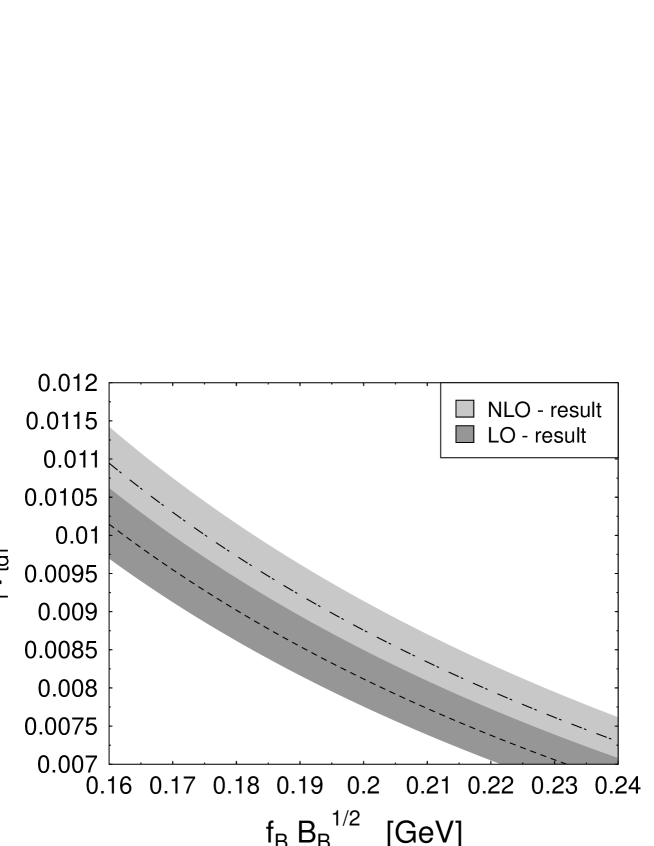
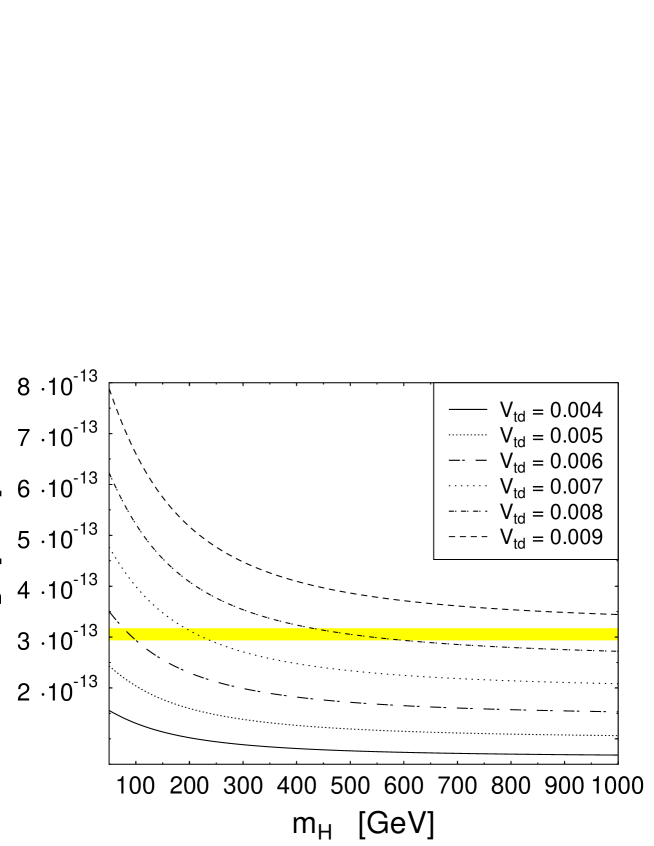
Figure 5: The CKM–element $V_{td}$ is plotted versus the B meson–decay constant times the square root of the B–parameter. The shaded areas represent the allowed values when errors of $\Delta m_{B}$ and $m_{t}$ are included. There is a small overlap between the LO- and the NLO region shown in the picture.

Figure 6: The mass splitting within the 2HDM including NLO-corrections for different values of $V_{td}$ and for $\tan\beta=1$. The top-quark mass is set to $m_{t}^{\rm pole}=175$ GeV. The shaded strip is the experimentally allowed region. The factor $f_{B}B_{B}^{1/2}$ is fixed to 0.2 GeV in this figure. The limit $m_{H}\rightarrow\infty$ yields the Standard Model results.

From Fig. 6 we can deduce that the difference between the LO–calculation and the corresponding NLO–calculation for $V_{td}$ is approximately $7\;\%$, when $m_{t}^{\rm pole}$ is used in the LO expression. Hence, the NLO–calculation enhances the result for the mass–splitting up to $15\;\%$. This can also be concluded by a direct comparison of $\eta_{LO}=\alpha_{S}(M_{W})^{6/23}$ and $\eta_{2}$ within the SM. We have found $\eta_{2}=0.4942$ and $\eta_{LO}=0.5751$.

If we consider an extended Higgs–sector within the framework of the 2HDM we have to decrease the related CKM–elements, to get an overlap between the allowed range for $\Delta m_{B}$ and the Higgs–mass. We recognize for example in Fig. 6 that we can not find a physical Higgs–boson with a mass smaller than 1 TeV for $V_{td}=0.0086$, assuming that the ratio of vacuum expectation values $\tan\beta=1$ and $f_{B}\,\sqrt{B_{B}}=0.2$ GeV. If we decrease $\tan\beta$ we have to decrease $V_{td}$ even more. Fig. 6 is in full agreement with Fig. 6 in the SM limit $m_{H}\rightarrow\infty$. If we assume $V_{td}=0.009$ and if we furthermore take into account the errors for $f_{B}\,\sqrt{B_{B}}$ and $m_{t}$ the 2HDM can not be distinguished from the SM for Higgs-boson masses larger than 1 TeV.

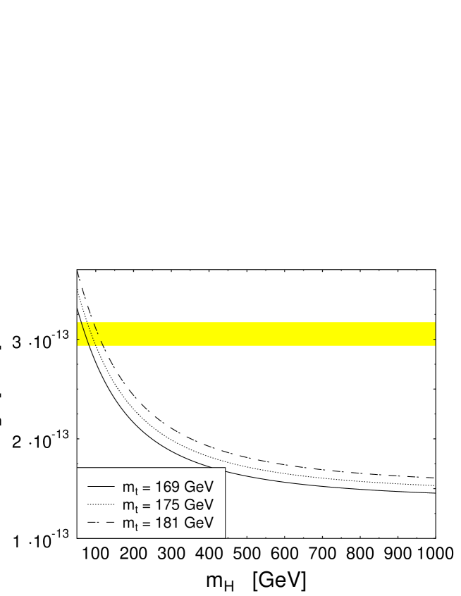
Figure 7: The mass splitting within the 2HDM for different values of the top-quark pole mass. In this figure, $V_{td}=0.009$, $\tan\beta=1$, $f_{B}B_{B}^{1/2}=0.2$ GeV.

In Fig. 7, it is indicated that we have a relatively sensitive relation between the top–quark mass and the possible Higgs–boson mass.

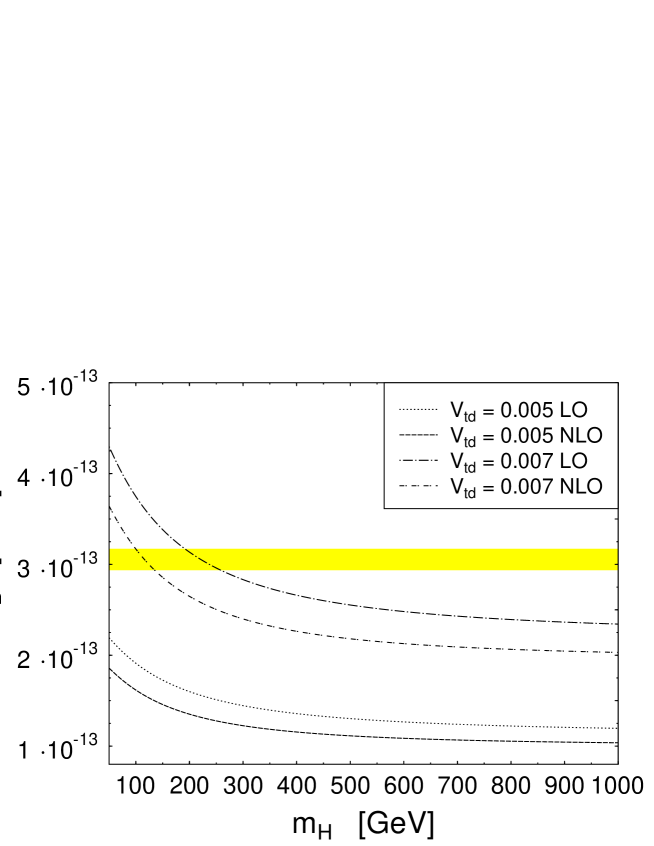
Figure 8: A comparison between LO calculations and NLO-calculations within the framework of the 2HDM. Here, $\tan\beta=1.25$, $f_{B}B_{B}^{1/2}=0.2$ GeV and $m_{t}^{\rm pole}=175$ GeV.

The comparison of NLO- and LO-calculation is shown in Fig. 8. We have plotted the mass-splitting over the Higgs-mass for two typical values of $V_{td}$ and a ratio of the vacuum expectation values $\tan\beta=1.25$. The difference between NLO- and LO-calculation approximately amounts to $18\;\%$.

5 Conclusions

We have calculated the $B^{0}\overline{B^{0}}$–mixing within Next–to–Leading–Order with the inclusion of two charged Higgs–bosons. The NLO calculation leads to an effect of approximately $7\;\%$ for $V_{td}$ in comparison to the LO calculation within the SM. This is indicated in Fig. 6.

We have verified that the scheme developed by Buras, Jamin, Weisz  [1, 13] for a proper separation of long and short distance effects in QCD remains valid in our 2HDM calculation. This can be considered as a good cross–check of the calculations presented here. The inclusion of NLO-corrections lowers the mass-splitting in the SM as well as in the 2HDM. We find, for example, a difference between the pure LO- and the NLO-calculations of approximately $18\;\%$ for $m_{H}=200$ GeV and $17.5\;\%$ for $m_{H}=400$ GeV. Hence the NLO-contributions plays an important role in the 2HDM as they correct the LO result by about $18\;\%$.

The inclusion of the two Higgs–bosons leads to an increase of the calculated amplitude, which depends on the mass and the vacuum expectation values of two Higgs doublets. In all practical calculations, the lower bound of the Higgs–boson mass was assumed to be 100 GeV and the upper bound was 1 TeV.

To obtain a mass–splitting within the experimental allowed region, it is necessary to decrease the CKM–matrix elements for small values of $\tan\beta$ and $m_{H}$. Our calculations are not valid for higher values of $\tan\beta$ (region near $\tan\beta=40$), because it is then necessary to introduce new operators.

In the limit of very heavy Higgs–bosons we verify the well–known results for the Standard Model.

Appendix A

A.1 Special functions

After carrying out the second integration, the dilogarithm or Spence function appears in our results. It is defined by

$${\rm Li}_{2}\,(x)=-\int_{0}^{x}\,dt\,\frac{\ln(1-t)}{t}=\sum_{n=1}^{\infty}\frac{x^{n}}{n^{2}}\,;\quad|x|<1\;\;.$$ (51)

The following useful relations hold

$${\rm Li}_{2}\,(1-x)+{\rm Li}_{2}\,(1-1/x)=-\frac{1}{2}\ln^{2}(x)\;\;,$$ (52)

$${\rm Li}_{2}\,(x)+{\rm Li}_{2}\,(1-x)=\frac{\pi^{2}}{6}-\ln(x)\,\ln(1-x)\;\;.$$ (53)

A.2 Inami–Lim functions and NLO in the SM

We list now the Inami–Lim functions and the well–known functions $L^{(i,SM)}(x_{W})$.

$$S_{WW}(x_{W}) = x_{W}\;\left(\frac{1}{4}+\frac{9}{4(1-x_{W})}-\frac{3}{2(1-x_{W})^{2}}-\frac{3x_{W}^{2}\ln(x_{W})}{2\,(1-x_{W})^{3}}\right)\;,$$ (54)

$$S_{HH}(x_{H}) = \frac{1}{\tan^{4}(\beta)}\,\frac{x_{H}\;x_{W}}{4}\left(\frac{1+x_{H}}{(1-x_{H})^{2}}+\frac{2x_{H}\ln(x_{H})}{(1-x_{H})^{3}}\right)\;,$$ (55)

$$2\;S_{WH}(x_{W},x_{H}) = \frac{1}{\tan^{2}(\beta)}\,\frac{x_{H}\;x_{W}}{4}\left(\frac{(2x_{W}-8x_{H})\ln(x_{H})}{(1-x_{H})^{2}(x_{H}-x_{W})}+\frac{6x_{W}\ln(x_{W})}{(1-x_{W})^{2}(x_{H}-x_{W})}\right.$$ (56)

$$\qquad\qquad\qquad\left.-\frac{8-2x_{W}}{(1-x_{H})(1-x_{W})}\right)\quad.$$

The function $S_{WH}(x_{W},x_{H})$ is obtained by including the charged would–be Goldstone bosons or in a more direct way, by choosing the unitary gauge for the $W$–boson right from the beginning.

The functions $L^{(i,SM)}$ can be decomposed as

$$L^{(i,SM)}(x_{W})=WW^{(i)}(x_{W})\,+\,2\,W\Phi^{(i)}(x_{W})\,+\,\Phi\Phi^{(i)}(x_{W})$$ (57)

where

$$WW^{(1)}(x_{W}) = WW^{(1)}_{tt}(x_{W})-2\;WW^{(1)}_{tu}(x_{W})+WW^{(1)}_{uu}(x_{W})\;\;,$$ (58)

$$WW^{(1)}_{tt}(x_{W}) = {(4\;x_{W}+38\;x_{W}^{2}+6\;x_{W}^{3})\;\ln(x_{W})\over{(x_{W}-1)}^{4}}+{(12\;x_{W}+48\;x_{W}^{2}+12\;x_{W}^{3})\;{\rm Li}_{2}(1-{1/x_{W}})\over{(x_{W}-1)}^{4}}$$ (59)

$$+{(24\;x_{W}+48\;x_{W}^{2})\;{\rm Li}_{2}(1-x_{W})\over{(x_{W}-1)}^{4}}-{{3+28\;x_{W}+17\;x_{W}^{2}}\over{(x_{W}-1)}^{3}}\;\;,$$

$$2\,WW^{(1)}_{tu}(x_{W}) = \frac{2\,(3\,+\,13\,x_{W})}{(x_{W}-1)^{2}}-\frac{2\,x_{W}\,(5\,+\,11\,x_{W})\;\ln(x_{W})}{(x_{W}-1)^{3}}$$ (60)

$$-\frac{12\,x_{W}\,(1\,+\,3\,x_{W})\;{\rm Li}_{2}(1-1/x_{W})}{(x_{W}-1)^{3}}-\frac{24\,x_{W}\,(1+x_{W}){\rm Li}_{2}(1-x_{W})}{(x_{W}-1)^{3}}\;,$$

$$WW^{(1)}_{uu}(x_{W}) = 3\;\;,$$ (61)

$$\Phi\Phi^{(1)}(x_{W}) = -\frac{x_{W}^{2}\,(7+52\,x_{W}-11\,x_{W}^{2})}{4\,(x_{W}-1)^{3}}+\frac{3\,x_{W}^{3}\,(4+5\,x_{W}-x_{W}^{2})\ln(x_{W})}{2\,(x_{W}-1)^{4}}$$ (62)

$$+\frac{3\,x_{W}^{3}\,(3+4\,x_{W}-x_{W}^{2}){\rm Li}_{2}(1-1/x_{W})}{(x_{W}-1)^{4}}+\frac{18\,x_{W}^{3}\,{\rm Li}_{2}(1-x_{W})}{(x_{W}-1)^{4}}\;\;,$$

$$2\;W\Phi^{(1)}(x_{W}) = \frac{4\,x_{W}^{2}\,(11+13\,x_{W})}{(x_{W}-1)^{3}}+\frac{2\,x_{W}^{2}\,(5\,+\,x_{W})(1-9\,x_{W})\ln(x_{W})}{(x_{W}-1)^{4}}$$

$$-\frac{24\,x_{W}^{2}\,(1+4\,x_{W}+x_{W}^{2}){\rm Li}_{2}(1-1/x_{W})}{(x_{W}-1)^{4}}-\frac{48\,x_{W}^{2}\,(1+2\,x_{W}){\rm Li}_{2}(1-x_{W})}{(x_{W}-1)^{4}}\;\;,$$

$$WW^{(8)}(x_{W}) = WW^{(8)}_{tt}(x_{W})-2\;WW^{(8)}_{tu}(x_{W})+WW^{(8)}_{uu}(x_{W})\;\;,$$ (64)

$$WW^{(8)}_{tt}(x_{W}) = {2\;x_{W}(4\;-\;3\;x_{W})\;\ln(x_{W})\over{(x_{W}-1)}^{3}}-{(12\;x_{W}-12\;x_{W}^{2}-8\;x_{W}^{3})\;{\rm Li}_{2}(1-{1/x_{W}})\over{(x_{W}-1)}^{4}}$$ (65)

$$+{(8-12\;x_{W}+12\;x_{W}^{2})\;{\rm Li}_{2}(1-\;x_{W})\over{(x_{W}-1)}^{4}}-{{(23\;-\;x_{W})}\over{(x_{W}-1)}^{2}}\;\;$$

$$2\;WW^{(8)}_{tu}(x_{W}) = {2\,(2\,-\,x_{W})\;\pi^{2}\over 3\,x_{W}}-{(8\,-\,5\;x_{W})\;\ln(x_{W})\over{(x_{W}-1)}^{2}}$$ (66)

$$-{(6\;x_{W}\,+\,4\;x_{W}^{2})\;{\rm Li}_{2}(1-{1/x_{W}})\over x_{W}\,{(x_{W}-1)}^{2}}+{(8\,+\,12\;x_{W}\,-\,6\;x_{W}^{2})\;{\rm Li}_{2}(1-x_{W})\over x_{W}\,{(x_{W}-1)}^{2}}$$

$$-{{15}\over{(x_{W}-1)}}\;\;,$$

$$WW^{(8)}_{uu}(x_{W}) = -23+{4\over 3}\;\pi^{2}\;\;,$$ (67)

$$\Phi\Phi^{(8)}(x_{W}) = -\frac{11\,x_{W}^{2}\,(1+x_{W})}{4\,(x_{W}-1)^{2}}+\frac{x_{W}^{3}\,(4\,-3\,x_{W})\ln(x_{W})}{2\,(x_{W}-1)^{3}}$$

$$+\frac{x_{W}^{3}\,(3-3\,x_{W}+2\,x_{W}^{2}){\rm Li}_{2}(1-1/x_{W})}{(x_{W}-1)^{4}}+\frac{x_{W}^{2}(2+3\,x_{W}-3\,x_{W}^{2}){\rm Li}_{2}(1-x_{W})}{(x_{W}-1)^{4}}\;\;,$$

$$2\;W\Phi^{(8)}(x_{W}) = \frac{30\,x_{W}^{2}}{(x_{W}-1)^{2}}+\frac{12\,x_{W}^{3}\ln(x_{W})}{(x_{W}-1)^{3}}-\frac{12\,x_{W}^{4}\,{\rm Li}_{2}(1-1/x_{W})}{(x_{W}-1)^{4}}$$ (69)

$$-\frac{12\,x_{W}^{2}\,(2\;-\,x_{W}^{2}){\rm Li}_{2}(1-x_{W})}{(x_{W}-1)^{4}}\;\;.$$

A.3 NLO in the extended Higgs sector

The $L^{(i,H)}$ can be decomposed in the following way

$$L^{(i,H)}(x_{W},x_{H})=\frac{2}{\tan^{2}(\beta)}\,WH^{(i)}(x_{W},x_{H})\,+\frac{2}{\tan^{2}(\beta)}\,\Phi H^{(i)}(x_{W},x_{H})+\,\frac{1}{\tan^{4}(\beta)}\,HH^{(i)}(x_{H})\;.$$

We list now the newly obtained results for the explicit QCD corrections in the extended Higgs sector:

$$HH^{(1)}(x_{i}) = \frac{x_{W}}{x_{H}}\Phi\Phi^{(1)}(x_{H})+6\;(\ln(x_{H})-\ln(x_{W}))\;\sum_{i=H,W}x_{i}\frac{\partial}{\partial x_{i}}\;S_{HH}(x_{i})\;\;,$$ (71)

$$2\;WH^{(1)}(x_{i}) = x_{W}\left(\frac{2\,x_{H}^{2}(13+3\,x_{H})\ln(x_{H})}{(x_{H}-1)^{3}(x_{H}-x_{W})}-\frac{2\,x_{H}\,(9+7\,x_{H}+7\,x_{W}-23\,x_{W}\,x_{H})}{(x_{W}-1)^{2}(x_{H}-1)^{2}}\right.$$ (72)

$$-\frac{2\,x_{H}^{2}(18\,-\,6\,x_{H}\,-44\,x_{W}+13\,x_{H}\,x_{W}+9\,x_{H}\,x_{W}^{2})\ln(x_{W})}{(x_{H}-1)^{2}(x_{W}-1)^{3}(x_{H}-x_{W})}$$

$$+\frac{2\,x_{H}\,x_{W}(5-27\,x_{W}+6\,x_{W}^{2}+6\,x_{H}\,x_{W}^{2})\ln(x_{W})}{(x_{H}-1)^{2}(x_{W}-1)^{3}(x_{H}-x_{W})}-\frac{24\,x_{H}^{2}\,\ln(x_{H})\,\ln(x_{W})}{(x_{H}-1)^{3}(x_{H}-x_{W})}$$

$$+\frac{24\,x_{H}^{2}\,\rm{Li}_{2}(1-1/x_{H})}{(x_{H}-1)^{2}(x_{H}-x_{W})}-\frac{24\,x_{H}\,x_{W}\,(1+x_{W})\,\rm{Li}_{2}(1-1/x_{W})}{(x_{W}-1)^{3}(x_{H}-x_{W})}$$

$$\left.-\frac{48\,x_{W}\,x_{H}\,\rm{Li}_{2}(1-x_{W})}{(x_{W}-1)^{3}(x_{H}-x_{W})}\right)\;\;,$$

$$2\;\Phi H^{(1)}(x_{i}) = x_{W}^{2}\left(\frac{x_{H}\,(31-15\,x_{H}\,-\,15\,x_{W}-x_{H}\,x_{W})}{2\,(x_{H}\,-\,1)^{2}\,(x_{W}\,-\,1)^{2}}-\frac{x_{H}\,(7+21\,x_{H}\,-\,12\,x_{H}^{2})\,\ln(x_{H})}{2\,(x_{H}\,-\,1)^{3}\,(x_{H}\,-\,x_{W})}\right.$$ (73)

$$+\frac{x_{H}\,(7\,-\,9\,x_{W}\,+\,36\,x_{W}^{2}\,-\,18\,x_{W}^{3})\,\ln(x_{W})}{2(x_{H}-1)^{2}(x_{H}-x_{W})(x_{W}-1)^{3}}$$

$$+\frac{x_{H}^{2}\,(8\,-\,36\,x_{W}\,+\,9\,x_{W}^{2}\,+\,3\;x_{W}^{3})\ln(x_{W})}{(x_{H}-1)^{2}(x_{H}-x_{W})(x_{W}-1)^{3}}$$

$$-\frac{x_{H}^{3}\,(11\,-\,45\,x_{W}\,+\,18\,x_{W}^{2})\,\ln(x_{W})}{2(x_{H}-1)^{2}(x_{H}-x_{W})(x_{W}-1)^{3}}+\frac{6\,x_{H}\,\ln(x_{H})\,\ln(x_{W})}{(x_{H}-1)^{3}(x_{H}-x_{W})}$$

$$-\frac{6\,x_{H}(1+x_{H}-x_{H}^{2}){\rm Li}_{2}(1-1/x_{H})}{(x_{H}-1)^{2}(x_{H}-x_{W})}$$

$$\left.+\frac{6\,x_{H}\,(1\,+\,2\,x_{W}^{2}\,-\,x_{W}^{3}){\rm Li}_{2}(1-1/x_{W})}{(x_{H}\,-\,x_{W})(x_{W}\,-\,1)^{3}}+\frac{12\,x_{H}\,{\rm Li}_{2}(1-x_{W})}{(x_{H}\,-\,x_{W})(x_{W}\,-\,1)^{3}}\right)\;\;,$$

$$HH^{(8)}(x_{i}) = \frac{x_{W}}{x_{H}}\Phi\Phi^{(8)}(x_{H})+6\;(\ln(x_{H})-\ln(x_{W}))\;S_{HH}(x_{i})\;\;,$$ (74)

$$2\;WH^{(8)}(x_{i}) = x_{W}\left(\frac{24x_{H}x_{W}{\rm Li_{2}}(1-x_{W})}{(x_{H}-x_{W})(x_{W}-1)^{2}}\right.$$ (75)

$$+\frac{6x_{H}^{2}(5x_{W}-x_{H}+3x_{W}^{2}x_{H}){\rm Li_{2}}(1-1/x_{W})}{(x_{H}-1)^{2}(x_{H}-x_{W})(x_{W}-1)^{2}x_{W}}$$

$$+\frac{6x_{H}(2x_{W}^{2}-10x_{H}x_{W}+x_{H}x_{W}^{2}){\rm Li_{2}}(1-1/x_{W})}{(x_{H}-1)^{2}(x_{H}-x_{W})(x_{W}-1)^{2}}$$

$$+\frac{6x_{H}^{2}(5x_{W}-x_{H}-8x_{W}^{2}+2x_{H}x_{W}^{2}){\rm Li_{2}}(1-x_{H})}{(x_{H}-1)^{2}(x_{H}-x_{W})(x_{W}-1)^{2}x_{W}}$$

$$+\frac{6(x_{W}^{2}-x_{H}x_{W}+2x_{H}^{2}x_{W}^{2}){\rm Li_{2}}(1-x_{H})}{(x_{H}-1)^{2}(x_{H}-x_{W})(x_{W}-1)^{2}}$$

$$+\frac{6x_{H}^{2}(-x_{H}+5x_{W}){\rm Li_{2}}(1-1/x_{H})}{(x_{H}-1)^{2}(x_{H}-x_{W})x_{W}}$$

$$-\frac{6x_{H}^{2}(5x_{W}-x_{H}-8x_{W}^{2}+2x_{H}x_{W}^{2}){\rm Li_{2}}(1-x_{H}/x_{W})}{(x_{H}-1)^{2}(x_{H}-x_{W})(x_{W}-1)^{2}x_{W}}$$

$$-\frac{6(x_{W}^{2}-x_{H}x_{W}+2x_{H}^{2}x_{W}^{2}){\rm Li_{2}}(1-x_{H}/x_{W})}{(x_{H}-1)^{2}(x_{H}-x_{W})(x_{W}-1)^{2}}$$

$$-\frac{6x_{H}(1-x_{H}-\ln(x_{H}))}{(x_{H}-1)^{2}(x_{W}-1)}+\frac{6x_{H}(2x_{W}-1)\ln(x_{W})}{(x_{H}-1)(x_{W}-1)^{2}}$$

$$+\frac{6x_{H}^{2}(5x_{W}-x_{H}-8x_{W}^{2})\ln(x_{H})\ln(x_{W})}{(x_{H}-1)^{2}(x_{H}-x_{W})(x_{W}-1)^{2}x_{W}}$$

$$\left.+\frac{12x_{H}^{2}(x_{H}x_{W}+x_{W}^{2})\ln(x_{H})\ln(x_{W})}{(x_{H}-1)^{2}(x_{H}-x_{W})(x_{W}-1)^{2}}\right)\;,$$

$$2\;\Phi H^{(8)}(x_{i}) = x_{W}^{2}\left(\frac{2\;x_{H}\;+\;2\;x_{W}\;-\;11\;x_{H}\;x_{W}}{2\;(x_{H}-1)\;(x_{W}-1)\;x_{W}}\right.$$ (76)

$$-\frac{(2\;x_{H}^{2}\;-\;7\;x_{H}\;x_{W}\;+\;2\;x_{H}^{2}\;x_{W}\;+\;2\;x_{W}^{2}\;+\;x_{H}\;x_{W}^{2})\ln(x_{H})}{2\;(x_{H}-1)^{2}\;(x_{H}-x_{W})\;(x_{W}-1)\;x_{W}}$$

$$-\frac{x_{H}\;(7\;-\;7\;x_{H}\;+\;4\;x_{W}\;-\;6\;x_{W}^{2})\;\ln(x_{W})}{2\;(x_{H}-1)\;(x_{H}-x_{W})\;(x_{W}-1)^{2}}$$

$$+\frac{(x_{H}^{2}\;+\;x_{W}^{2}\;-\;3\;x_{H}^{2}\;x_{W}^{2})\;\ln(x_{W})}{(x_{H}-1)\;(x_{H}-x_{W})\;(x_{W}-1)^{2}\;x_{W}}$$

$$-\frac{x_{H}^{2}\;(4\;-\;6\;x_{W}\;+\;3\;x_{H}\;x_{W})\;\ln(x_{H})\;\ln(x_{W})}{(x_{H}-1)^{2}\;(x_{H}-x_{W})\;(x_{W}-1)^{2}\;x_{W}}$$

$$+\frac{x_{H}\;(x_{H}^{2}\;-\;3\;x_{W}^{2}\;+\;6\;x_{W}^{3}\;-\;3\;x_{W}^{4})\;\ln(x_{H})\;\ln(x_{W})}{(x_{H}-1)^{2}\;(x_{H}-x_{W})\;(x_{W}-1)^{2}\;x_{W}^{2}}$$

$$-\frac{x_{H}\;(3\;x_{W}^{2}\;+\;2\;x_{H}\;x_{W}\;(2\;+\;x_{W})\;-\;x_{H}^{2}\;(1\;+\;2\;x_{W}))\;{\rm Li}_{2}(1-1/x_{H})}{(x_{H}-1)^{2}\;(x_{H}-x_{W})\;x_{W}^{2}}$$

$$-\frac{(4\;x_{H}\;x_{W}\;-\;6\;x_{H}^{2}\;x_{W}\;+\;3\;x_{H}^{2}\;x_{W}^{2}\;-\;x_{W}^{2}){\rm Li}_{2}(1-x_{H})}{(x_{H}-1)^{2}\;(x_{H}-x_{W})\;(x_{W}-1)^{2}\;x_{H}}$$

$$-\frac{(4\;x_{H}^{2}\;x_{W}\;-\;6\;x_{H}^{2}\;x_{W}^{2}\;-\;x_{H}^{3}\;+\;3\;x_{H}^{3}\;x_{W}^{2}){\rm Li}_{2}(1-x_{H})}{(x_{H}-1)^{2}\;(x_{H}-x_{W})\;(x_{W}-1)^{2}\;x_{W}^{2}}$$

$$+\frac{2\;x_{H}^{2}\;(6\;-\;x_{W}^{2}\;-\;3\;x_{H}\;+\;x_{W}\;x_{H})\;{\rm Li}_{2}(1-1/x_{W})}{(x_{H}-1)^{2}\;(x_{H}-x_{W})\;(x_{W}-1)^{2}}$$

$$-\frac{x_{H}\;(3\;x_{W}^{2}\;+\;4\;x_{H}\;x_{W}\;-\;x_{H}^{2})\;{\rm Li}_{2}(1-1/x_{W})}{(x_{H}-1)^{2}\;(x_{H}-x_{W})\;(x_{W}-1)^{2}\;x_{W}^{2}}$$

$$+\frac{(4\,x_{H}\;x_{W}\;-\;6\;x_{H}^{2}\;x_{W}\;+\;3\;x_{H}^{2}\;x_{W}^{2}\;-\;x_{W}^{2}){\rm Li}_{2}(1-x_{H}/x_{W})}{(x_{H}-1)^{2}\;(x_{H}-x_{W})\;(x_{W}-1)^{2}\;x_{H}}$$

$$+\frac{x_{H}^{2}(4\;x_{W}\;-\;6\;x_{W}^{2}\;-\;x_{H}\;+\;3\;x_{H}\;x_{W}^{2}){\rm Li}_{2}(1-x_{H}/x_{W})}{(x_{H}-1)^{2}\;(x_{H}-x_{W})\;(x_{W}-1)^{2}\;x_{W}^{2}}$$

$$\left.-\frac{6\;x_{H}\;{\rm Li}_{2}(1-x_{W})}{(x_{H}-x_{W})\;(x_{W}-1)^{2}}\right)\;.$$

We have used the capital $W$, $\Phi$ and $H$ to label the W–boson, the charged would–be Goldstone boson and the physical Higgs–boson, respectively, i.e. $W\Phi$ denotes a diagram with one internal $W$–boson and one internal unphysical scalar.

Figure 1: Box diagrams for the $B^{0}\overline{B^{0}}$–mixing in the framework of 2HDM. We have also taken into account crossed diagrams, which are related to the original ones by a Fierz–transformation.

Figure 2: QCD-corrections to the effective four quark interaction. They are needed in the calculation of the anomalous dimension at LO and for the correct separation of long and short distance contributions.

a)	b)
c)	d)
e)	f)

Figure 3: Diagrams for the NLO-calculation in the SM, which are convergent in the limit of vanishing external masses. Additional diagrams with one Higgs-boson and two Higgs-bosons have to be calculated in the 2HDM. Furthermore, we have to consider crossed diagrams.

g)	h)
i)	j)
k)

Figure 4: Diagrams for the NLO-calculation in the SM, in which infrared divergences appear when one sets external masses to zero. The last diagram is the so-called double-penguin, which does not contribute to the mixing at the leading order in $(m_{B}/m_{W})^{2}$. Additional diagrams with one Higgs-boson and two Higgs-bosons have to be calculated in the 2HDM. Furthermore, we have to consider crossed diagrams.