NUCLEAR SHADOWING AND RHO PHOTOPRODUCTION

Abstract

Rho photoproduction on complex nuclei is re-examined using a generalised vector dominance model which succesfully predicts the oberved nuclear shadowing in real photoabsorption and deep inelastic scattering. This model is shown to give a good fit to rho photoproduction data on both nucleons and complex nuclei, in which the disagreement between the measured $\gamma-\rho$ coupling and the $\gamma-\rho$ coupling required by the simple vector dominance model is eliminated. The $\rho N$ total cross-sections required are similar to those predicted by the additive quark model; and the magnitude of the correction to simple vector dominance is consistent with that inferred from the analysis of real photoabsorption and deep inelastic scattering.

I Introduction

In this paper, we address the apparent contradiction between the well-known simple vector dominance(SVD) treatment of rho photoproduction; and the very succesful generalized vector dominance(GVD) treatment of nuclear shadowing in real photoabsorption and deep inelastic scattering.

In 1989, one of us [1] pointed out that the observed qualitative features of nuclear shadowing in deep inelastic scattering [2] are simply and naturally accounted for in a generalized vector dominance(GVD) model [3] which can be shown to be dual to the parton model [1, 4]. The crucial feature of this model, in the context of shadowing, is that the cross-sections $\sigma_{VN}$ for scattering a sequence of hadronic vector states $V=\rho,\rho^{\prime},\ldots$ from nucleons are required to be approximately independent of their mass $m_{V}$. This then leads to approximate scaling behaviour for shadowing and a rapid decrease in the effect as $x$ increases from zero, as observed in the data [5]. Somewhat later, in 1993, the same model was shown [6] to give an accurate quantitative account of both real photoabsorption on nuclei [7] and the precise shadowing data that had by then become available for virtual photons [8].

The above GVD model is consistent with the fundamental QCD picture of strong interactions in appropriate kinematic regions. It has implications for rho photoproduction, because it necessarily includes substantial contributions from “non-diagonal” diffraction dissociation processes of the type $VN\rightarrow V^{\prime}N$ in addition to “diagonal” elastic processes of the type $VN\rightarrow VN$. This feature is also implied by duality with the parton model [1, 4]. In addition, without such processes, the cross-sections $\sigma_{VN}$ would be forced to decrease rapidly with mass $m_{V}$ to maintain approximate scaling in the nucleon structure functions; and shadowing would die away as $Q^{2}$ increases at fixed $x$, in contradiction to approximate scaling for the nuclear structure functions. These diffraction dissociation processes also contribute to $rho$-photoproduction, as illustrated in Figure 1, giving significant corrections to the well-known predictions of the simple vector dominance(SVD) model. This result is potentially a serious problem, since rho photoproduction on both nucleons and nuclei has long been regarded as the outstanding success of the SVD model; and if the agreement between the SVD predictions and the data were really good, it would clearly undermine the above GVD approach. However, as Donnachie and Landshoff [11] have recently pointed out, the SVD predictions for the cross-sections on nucleons are lie approximately 16$\%$ above the measured values.

In this paper we shall investigate rho photoproduction on both nucleons and nuclei within the framework of the GVD model used to successfully account for shadowing in real and virtual photoabsorption. The aims are to see whether model can resolve the discrepancy between the predictions of SVD and the nucleon data, while retaining the successful predictions of SVD for the $A$ dependence on nuclei; and if so, whether sign and magnitude of the diffraction dissociation terms required by the rho photoproduction data are consistent with those required by the real photoabsorption and structure function data.

II Rho photoproduction on nucleons

We begin by reviewing rho photoproduction on nucleons

$$\gamma+N\rightarrow\rho+N\hskip 56.9055pt(N=n,\,p)$$

-a topic in which there is renewed interest because of recent data from HERA [12, 13]. At high energies, the process is usually described in terms of the SVD model of Figure 1, leading to the well-known relation

$$f_{\gamma\rho}(s,t=0)=\frac{e}{f_{\rho}}f_{\rho\rho}(s,t=0)\hskip 42.67912pt(SVD)$$ (1)

where $f_{ab}$ is the scattering amplitude for $a+N\rightarrow b+N$ and $f_{\rho}$ is the $\gamma-\rho$ coupling. Using the optical theorem, this gives

$$\frac{d\,\sigma}{d\,t}(s,t=0)=\alpha\frac{4\,\pi}{f_{\rho}^{2}}\sigma_{\rho N}^{2}\,[1+\eta^{2}]\hskip 42.67912pt(SVD)$$ (2)

for the forward differential cross-section, where $\sigma_{\rho N}$ is the total cross-section for $\rho\,N$ scattering and $\eta$ is the ratio of the real to imaginary part of the forward $\rho\,N$ scattering amplitude. The value of $\sigma_{\rho N}$ is usually taken from the additive quark model prediction

$$\sigma_{\rho\,N}=\frac{1}{2}\left[\sigma_{\pi^{+}\,N}+\sigma_{\pi^{-}\,N}\right]\;;$$ (3)

and $\eta$ is estimated from Regge pole ideas.

The resulting SVD prediction (2, 3) was long ago compared with experimental photoproduction data on protons available at energies below 20 GeV to yield a value [14]

$$\frac{f_{\rho}^{2}}{4\,\pi}=2.44\pm 0.12\;.$$ (4)

for the coupling constant. At the time, this simple picture was consistent with the corresponding SVD analysis of vector meson photoproduction on nuclei [15, 16] and with the then not very precisely known value of the $\gamma-\rho$ coupling obtained directly from the measured decay width $\Gamma(\rho\rightarrow e^{+}e^{-})$. Since then events have moved on and it is important to check whether this consistency still obtains. The precision of the measured decay width $\Gamma(\rho\rightarrow e^{+}e^{-})$ has greatly increased [17], and now gives

$$\frac{f_{\rho}^{2}}{4\,\pi}=2.01\pm 0.10\;,$$ (5)

which is not in good agreement with the phenomenological value (4). This problem is confirmed by a recent comparison [11] incorporating higher energy photoproduction data [12, 18], which finds that the SVD prediction (2, 3) obtained using the directly measured coupling (5) lies on average about 16 % above the measured data.

The discrepancy between the experimental data and the SVD approximation presumably arises from contributions which are neglected in this approximation. There are two obvious possibilities. The first is finite width effects associated with the $\rho^{0}\rightarrow\pi^{+}\;\pi^{-}$ decay channel, as shown in Figure 2. Detailed calculations show that this is very unlikely, since the correction arising from the modification to the rho propagator is largely cancelled by corrections arising from the pion scattering terms [19].

The second possibility is to attribute the discrepancy to neglected contributions from higher mass vector states, leading to the generalized vector dominance(GVD) model shown in Figure 1. In principle many states could contribute, but in practice only the lightest states are expected to be important, since the diffraction dissociation amplitudes $f(\rho^{\prime}N\rightarrow\rho N)$, and to a lesser degree the couplings $(e/f_{\rho^{\prime}})$, are expected to decrease rapidly with increasing mass $m_{\rho^{\prime}}$ [20]. Hence it is reasonable to approximate these contributions with that of a single effective $\rho^{\prime}$ state, when the SVD prediction (1) is replaced by

$$f_{\gamma\rho}=\frac{e}{f_{\rho}}f_{\rho\rho}+\frac{e}{f_{\rho^{\prime}}}f_{\rho^{\prime}\rho}\hskip 42.67912pt(GVD)\,.$$ (6)

This form also follows directly from the generalised vector dominance model [3] used to successfully predict the observed shadowing effects in both real photoabsorption and deep inelastic scattering on nuclei [6]. We shall not discuss this model further, but just use it to specify the properties of the effective $\rho^{\prime}$, which are

$$m_{\rho^{\prime}}^{2}=3m_{\rho}^{2}\ \ \ \ \ \ \ \ \ \ \ f_{\rho^{\prime}}=m_{\rho^{\prime}}f_{\rho}/m_{\rho}$$ (7)

together with

$$f_{\rho^{\prime}\rho^{\prime}}=f_{\rho\rho}\hskip 56.9055ptf_{\rho^{\prime}\rho}=f_{\rho\rho^{\prime}}=-\epsilon f_{\rho\rho}$$ (8)

for the forward scattering amplitudes, where

$$\epsilon\approx 0.2\;.$$ (9)

Here, we shall retain (6 - 8) but treat $\epsilon$ as a free parameter to be determine by the $\rho$-photoproduction data. The forward cross-cross-section is then given by

$$\frac{d\,\sigma}{d\,t}(s,t=0)=\alpha\frac{4\,\pi}{f_{\rho}^{2}}\sigma_{\rho N}^{2}\,[1+\eta^{2}]\left[1-\epsilon\frac{m_{\rho}}{m_{\rho^{\prime}}}\right]^{2}\hskip 28.45274pt(GVD).$$ (10)

For fixed $\sigma_{\rho N}$ and $\eta$, the results of SVD with the effective coupling (4) are reproduced by GVD with the physical coupling (5) and $\epsilon=0.160\pm 0.055$, which is in good agreement with the value (9) quoted above.

We thus have two accounts of the data on $\rho$ photoproduction on protons: either the SVD model in which the $\gamma-\rho$ coupling is adjused to fit the data; or the GVD model in which this coupling is fixed at its measured value and and the parameter $\epsilon$ is adjusted to fit the data. The latter is more compatible with the ideas used to understand shadowing in nucleon structure functions, but its predictions for $\rho$ photoproduction on nuclei have never been examined. It is our aim to remedy this omission and discuss the implications of the results.

III Rho photoproduction on nuclei

In the generalised vector dominance model, an incident photon may convert into a a whole sequence of isovector, vector mesons $V=\rho,\rho^{\prime},\rho^{\prime\prime},\ldots$ while traversing a nucleus. According to Glauber theory [21] [22], this possibility is dealt with by introducing appropriate optical potentials $U_{\gamma V}$, $U_{\gamma\gamma}$, $U_{VV}$, $U_{VV^{\prime}}$, which characterise the features of the scatterer, where $V,V^{\prime}$ are arbitrary members of the vector meson sequence. The resulting wave equation then reads

$$\left[\left(\begin{array}[]{cc}\bigtriangledown^{2}+k_{\gamma}^{2}&{\bf 0}\\ {\bf 0}&\cal V\end{array}\right)-\left(\begin{array}[]{cc}U_{\gamma\gamma}&\mbox{$\boldmath U_{\gamma}^{T}$}\\ \mbox{$\boldmath U_{\gamma}$}&\cal U\end{array}\right)\right]\left(\begin{array}[]{c}\Psi_{\gamma}\\ {\bf\Psi}\end{array}\right)=0$$ (11)

where

$$\left(\cal V\right)_{VV^{\prime}} = \delta_{VV^{\prime}}(\bigtriangledown^{2}+k^{2}_{V})$$ (12)

$$\left(\cal U\right)_{VV^{\prime}} = U_{VV^{\prime}}$$ (13)

$$\left({\bf\Psi}\right)_{V} = \psi_{V}$$ (14)

$$\left(\mbox{$\boldmath U_{\gamma}$}\right)_{V} = U_{\gamma V}\ .$$ (15)

In this paper we restrict ourselves to two hadronic channels $\rho,\rho^{\prime}$ and use the eikonal approximation

$$\Psi_{\gamma}=\Phi_{\gamma}e^{ik_{\gamma}z}\ \ \ \ \Psi_{\rho,\rho^{\prime}}=\Phi_{\rho,\rho^{\prime}}e^{ik_{\rho,\rho^{\prime}}z}$$ (16)

where the reduced wave functions $\Phi_{\gamma}$, $\Phi_{\rho}$, $\Phi_{\rho^{\prime}}$ are assumed to vary slowly enough for all second derivatives to be discarded. Furthermore, since we are only interested in the photoproduction amplitude, it is sufficient to work to order $\cal O(\sqrt{\alpha})$ only. Hence, when the photon wavefunction occurs multiplied by factors $U_{\gamma\rho}$ or $U_{\gamma\gamma}$, which are already of this or higher order, we can replace it by the incident photon wave $\Psi_{\gamma}=e^{ik_{\gamma}z}$. With these approximations, the reduced wavefunctions of the vector mesons satisfy the coupled differential equations

$$\ \ \!\frac{d}{dz}\Phi_{\rho}({\bf b},z)=-\frac{i}{2k_{\rho}}\left(U_{\gamma\rho}e^{iq_{\|_{\gamma\rho}}z}+U_{\rho\rho}\Phi_{\rho}({\bf b},z)+U_{\rho\rho^{\prime}}\Phi_{\rho^{\prime}}({\bf b},z)e^{iq_{\|_{\rho\rho^{\prime}}}z}\right)$$ (17)

$$\frac{d}{dz}\Phi_{\rho^{\prime}}({\bf b},z)=-\frac{i}{2k_{\rho^{\prime}}}\left(U_{\gamma\rho^{\prime}}e^{iq_{\|_{\gamma\rho^{\prime}}}z}+U_{\rho^{\prime}\rho^{\prime}}\Phi_{\rho^{\prime}}({\bf b},z)+U_{\rho^{\prime}\rho}\Phi_{\rho}({\bf b},z)e^{iq_{\|_{\rho^{\prime}\rho}}z}\right)$$ (18)

where the space coordinates are parameterized through the z-coordinate in the direction of the incident photon wave and the impact parameter b in the plane perpendicular to the z-axis. The expressions $q_{\|_{ij}}=k_{i}-k_{j}$ denote the minimal longitudinal momentum transfer between particle i and j, where i and j are members of the set $\gamma,\ \rho,\ \rho^{\prime}$.

A Optical potentials and nuclear densities.

The optical potentials are given by [21]

$$U_{ij}=-4\pi f_{ij}\ n({\bf b},z)\ \ \ \ \ U_{ij}=U_{ji}$$ (19)

where the forward scattering amplitudes on nucleons $f_{ij}$ are given by eqs.(6 - 8) together with the GVD analogue of (6) for the $\rho^{\prime}$:

$$f_{\gamma\rho^{\prime}}=\frac{e}{f_{\rho}}f_{\rho\rho^{\prime}}+\frac{e}{f_{\rho^{\prime}}}f_{\rho^{\prime}\rho^{\prime}}\,.$$ (20)

Two different models [22] are employed for the nuclear density $n({\bf b},z)$, depending on the size of the nucleus.

• $A>16$
  For heavy nuclei, $A>16$, we use a Fermi gas-like mass distribution of the form

  $$n({\bf r})=n_{W}\left(1+\exp\left(\frac{r-R_{W}}{c}\right)\right)^{-1}\ .$$ (21)

  where the ‘skin-thickness’$\;c=0.545$ fm. The Woods-Saxon radius $R_{W}$ is given as the solution of the equation

  $$A\ f(R_{W})=n_{W}\equiv A_{\mbox{Pb}}\ f(R_{\mbox{Pb}})$$ (22)

  corresponding to a fixed central density $n_{W}$, where

  $$f(\rho)=\left(\frac{3}{4\pi\rho^{3}}\right)\left(1+\pi^{2}\frac{c^{2}}{\rho^{2}}\right)^{-1}$$ (23)

  and $R_{Pb}=6.626$ fm.

• $A<16$
  For light nuclei, the Woods-Saxon formula is not a good description. Instead we use a shell model (harmonic oscillator) density, given by

  $$n(r)=n_{s}\left(1+\delta\left(\frac{r}{R_{S}}\right)^{2}\right)\exp\left(-\left(\frac{r}{R_{S}}\right)^{2}\right)$$ (24)

  where

  $$\delta=\frac{A-4}{6}\ \ \ \ \ \ \ \ \ \ \ \ \ \ n_{s}=\frac{2A}{2+3\delta}\left(\sqrt{\pi}R_{S}\right)^{-3}$$ (25)

  and the shell model radius $R_{S}=0.708\,\mbox{A}^{\frac{1}{3}}$ fm.

Finally, to take two-body correlations into account, we modify the nuclear density functions by the replacement [23]

$$n({\bf r})\ \longrightarrow\ n({\bf r})\left(1+\frac{1}{2}\ l_{c}\ \sigma_{\rho N}\ n({\bf r})\ \left(\frac{n({\bf r}=0)}{n({\bf r})}\right)^{-\frac{1}{3}}\right)$$ (26)

where the two body correlation length $l_{c}$ =0.3 fm.

B Evaluation of the cross-sections

To evaluate the cross-section for $\rho$ photoproduction on heavy nuclei, we need to solve (17, 18) with the initial conditions

$$\Phi_{\rho}({\bf b},z=-\infty)=\Phi_{\rho^{\prime}}({\bf b},z=-\infty)=0$$ (27)

corresponding to incident photons. The forward differential cross section is then given by

$$\frac{d\sigma}{dt}(t=0)\ =\ \frac{\pi}{k_{\rho}^{2}}\ |F_{\gamma\rho}(0)|^{2}\ .$$ (28)

where the forward scattering amplitude $F_{\gamma\rho}$ is related to the “profile function”

$$\Gamma_{\rho}({\bf b})=-\lim_{z\rightarrow\infty}\Phi_{\rho}({\bf b},z)\ .$$ (29)

by the standard result [21]

$$F_{\gamma\rho}(0)=i\,k_{\rho}\int_{0}^{\infty}db\ b\ \Gamma(b)\;.$$ (30)

From (17, 18), it is clear that the reduced wavefunctions only vary with $z$ at fixed impact parameter ${\bf b}$ in regions where optical potentials (19) are non-zero. Since the nuclear densities fall off very rapidly beyond the nuclear radii, we neglect such variations for $|z|>4R_{W}$, measured from the centre of the nucleus. The initial conditions (27) are imposed at $z=-4R_{W}$ and (17, 18) are integrated up to $z=+4R_{W}$ at fixed impact parameter ${\bf b}$ using a fourth-order Runge-Kutta algorithm with an adaptive stepsize control. The profile function is then evaluated at $z=+4R_{W}$ rather than infinity and used to compute cross-sections, which are compared with experiment in the concluding section. Typical results for the reduced wavefunction $\Phi_{\rho}$ and the profile function $\Gamma(b)$ are shown in Fig. 3 and Fig. 4 respectively, verifying the assumed disappearance of structure by $4R_{W}$.

C A simple approximation

Before comparing with experiment, we comment briefly on an approximation that gives a useful check on our numerical solutions. In the SVD model, the eikonal equation (17) with $f_{\rho\rho^{\prime}}=0$ can be integrated explicitly and this result is easily generalized to the coupled channel GVD case (17, 18) in the high energy limit when

$${\rm e}^{iq_{\|_{\rho\rho^{\prime}}}z}=1\;.$$ (31)

This approximation has been used to analyse the $\rho$ photoproduction data by Kroker [24] giving, for example, a value $\sigma_{\rho N}=29.0\pm 1.2$ mb corresponding to an incident photon energy of 6.1 GeV. The corresponding prediction for the nuclear cross-sections is shown in Figure 5, where it is compared both to the data and to our “exact” predictions for the same parameter values. In fact

$${\rm e}^{iq_{\|_{\rho\rho^{\prime}}}z}=i\hskip 28.45274pt{\rm for}\hskip 28.45274ptE_{\gamma}=6.1\,GeV,\;\;\;z\approx 3\,f\;.$$

Since $z=3$ f is well within a large nucleus for small impact parameters $b\approx 0$, it is clear that (31) is quantitatively unreliable at the energies where data currently exists. We shall not consider it further, except to note that our numerical solutions reproduce both the standard SVD predictions and Kroker’s approximate results [24] when we impose $f_{\rho\rho^{\prime}}=0$ or (31) respectively.

IV Results and Conclusions

In this section we present the results of an optical model analysis of the experimental data on complex nuclei using the GVD model described. At each energy the cross-sections depend on four parameters:

$$\frac{f_{\rho}^{2}}{4\pi}\hskip 14.22636pt\sigma_{\rho N}\hskip 14.22636pt\epsilon\hskip 14.22636pt\eta\;.$$

Our strategy is to fix the coupling $f_{\rho}$ at its measured value (5) and the phase ratio $\eta$ at the values implied by the Regge pole parameterization

$$f_{\rho\rho}(s,t=0)=g_{P}\frac{-1-e^{-\pi\alpha_{P}}}{\sin(\pi\alpha_{P})}s^{\alpha_{P}}+g_{R}\frac{-1-e^{-\pi\alpha_{R}}}{\sin(\pi\alpha_{R})}s^{\alpha_{R}}$$ (32)

where the subscripts P and R denote the pomeron and Regge contributions respectively and the constants $\alpha_{P},\;\alpha_{R},\;g_{P}$ and $g_{R}$ are fixed by assuming the additive quark model relation $f_{\rho N}=f_{\pi N}$ together with the Donnachie-Landshoff fit [25] to $\pi N$ scattering data. The remaining parameters $\sigma_{\rho N}$ and $\epsilon$ are then determined by fitting to the $\rho$-photoproduction data. First, however, we summarise the earlier SVD results and the data available.

We are only interested in data at high enough energies for the phase parameter $\eta$ to be small and reasonably well estimated by conventional Regge pole ideas. The most precise data on complex nuclei at such energies was obtained by a DESY-MIT group [15] at a photon energy of 6.6 GeV and by a Cornell group[16]) at 6.1, 6.5 and 8.8 GeV. The latter group also presented results on protons and deuterium, giving measurements of the single nucleon cross-section from the same experiment. They then carried out an SVD analysis of their own nucleon and nuclear cross-sections, assuming input phases $\eta$ which are somewhat larger than those given by (32), and treating both the $\gamma-\rho$ coupling and the $\rho N$ total cross-section as parameters to be fitted to the data. Their results are summarised in Table I. This analysis was repeated by Kroker [24] with phases close to those assumed here, and combining both the Cornell and DESY-MIT data at 6.5/6.6 GeV. The resulting parameter values are given in Table II, and the corresponding prediction is compared with the data at 6.1 GeV in Figure 5. Since both analyses used exactly the same data at 6.1 and 8.8 GeV, a comparison of Tables I and II at these energies explicitly confirms the insensitivity of the results to small changes in the input phases.

Here, we repeat this anaysis using the GVD model described above, using the experimental $\gamma-\rho$ coupling value (5). Since this involves non-trivial numerical computation, we simplify the determination of the two free parameters $\epsilon$ and $\sigma_{\rho N}$ by requiring that the GVD predictions exactly reproduce the succesful SVD results on single nucleons; and then determine the remaining parameter by a fit to the nuclear data. Satisfactory fits are obtained in this way at all three energies 6.1,6.5 and 8.8 GeV as shown in Figures 6, 7 and 8. The corresponding parameter values are shown in Table III. As can be seen, the values obtained for the off-diagonal parameter $\epsilon$ at the three energies are consistent with each other and with the value (9) required by the successful treatment of nuclear shadowing in real photoabsorption and deep inelastic scattering [6]. The central values for $\sigma_{\rho N}$ are slightly larger than those obtained in the SVD model fits(cf. Table II), but are consistent within the quoted uncertainties arising from the errors on the experimental data. They are also slightly larger than, but in qualitative agreement with, the crude prediction (3) of the aditive quark model, which gives $\sigma_{\rho N}\approx 27,27,26$ mb at $E_{\gamma}=6.1,6.5,8.8$ GeV respectively.

In short, the model is in good agreement with the data on $\rho$-photoproduction on both nucleons and nuclei, with a $\gamma-\rho$ coupling consistent with that measured in electron-positron annihihation. The form and magnitude of the correction to simple vector dominance, characterized by the parameter $\epsilon$, is consistent with that required by the succesful description of shadowing in both real photoabsorption and deep inelastic scattering.

TABLE CAPTIONS

Table I Parameters of the SVD fits of the Cornell group [16] to their own data, together with the input values of the phase ratio $\eta$.

Table II Parameters of the SVD fits of Kroker [24] to the Cornell data [16] at 6.1 and 8.8 GeV, and the combined Cornell and DESY-MIT data [15] at 6.5 GeV, together with the input values of the phase ratio $\eta$.

Table III Parameters of our optical model GVD fits to the Cornell data [16] at 6.1 and 8.8 GeV, and the combined Cornell and DESY-MIT data [15] at 6.5 GeV. The phase ratio $\eta$ is given by (29) and the $\gamma-\rho$ coupling is fixed at its measured value (5).

FIGURE CAPTIONS

Figure 1 The SVD diagram for $\rho^{0}$ photoproduction(left), together with the GVD corrections to it arising from diffraction dissociation terms(right).

Figure 2 Finite width corrections to SVD associated with the $2\pi$- channel. The first diagram is a propagator correction, the second a $2\pi$- scattering contribution.

Figure 3 The reduced wave function $\Phi_{\rho}$ calculated at zero impact parameter for lead nuclei at 6.1 GeV. The parameters are those of our final fit(see Table III below.)

Figure 4 The profile function $\Gamma_{\rho}$ calculated for lead nuclei at 6.1 GeV. The parameters are those of our final fit(see Table III below).

Figure 5 Comparison between different theoretical predictions and the complex nuclei data for $E_{\gamma}$=6.1 GeV: the SVD-prediction assuming the parameter values of Table II (dashed dotted line); the GVD solution in the approximation (28) using the parameter values given by Kroker [24] (dashed line); and the full GVD prediction using the same parameters (solid line).

Figure 6 The optical moddel GVD fit to the complex nuclei data at 6.1 GeV, corresponding to the parameters of Table III.(The deuteron data point shown is not included in the fit for obvious reasons.)

Figure 7 The optical model GVD fit to the complex nuclei data at 6.5 GeV, corresponding to the parameters of Table III.(The deuteron data point shown is not included in the fit for obvious reasons.)

Figure 8 The optical model GVD fit to the complex nuclei data at 8.8 GeV, corresponding to the parameters of Table III.(The deuteron data point shown is not included in the fit for obvious reasons.)

$E_{\gamma}$ [MeV]	$\alpha_{\eta}$	$\sigma_{\rho N}\ \$[mb]	$f_{\rho}^{2}/4\pi$
6.1	-0.27	27.5$\pm$1.1	2.48$\pm$0.16
6.5	-0.27	27.9$\pm$1.3	2.60$\pm$0.20
8.8	-0.24	25.9$\pm$1.0	2.52$\pm$0.16

TABLE I.: Parameters of the SVD fits of the Cornell group [16] to their own data, together with the input values of the phase ratio $\eta$.

$E_{\gamma}$ [MeV]	$\eta$	$\sigma_{\rho N}\ \$[mb]	$f_{\rho}^{2}/4\pi$
6.1	-0.24	27.5$\pm$1.1	2.44$\pm$0.16
6.5	-0.23	26.7$\pm$2.0	2.28$\pm$0.10
8.8	-0.20	26.2$\pm$1.0	2.52$\pm$0.16

TABLE II.: Parameters of the SVD fits of Kroker [24] to the Cornell data [16] at 6.1 and 8.8 GeV, and the combined Cornell and DESY-MIT data [15] at 6.5 GeV, together with the input values of the phase ratio $\eta$.

$E_{\gamma}$ [MeV]	$\eta$	$\sigma_{\rho N}\ \$[mb]	$f_{\rho}^{2}/4\pi$	$\epsilon$
6.1	-0.26	28.1$\pm$1.1	2.01	0.19$\pm$0.050
6.5	-0.24	28.4$\pm$2.0	2.01	0.21$\pm$0.035
8.8	-0.20	27.9$\pm$1.0	2.01	0.28$\pm$0.046

TABLE III.: Parameters of our optical model GVD fits to the Cornell data [16] at 6.1 and 8.8 GeV, and the combined Cornell and DESY-MIT data [15] at 6.5 GeV. The phase ratio $\eta$ is given by (29) and the $\gamma-\rho$ coupling is fixed at its measured value (5).

FIG. 1.: The SVD diagram for $\rho^{0}$ photoproduction(left), together with the GVD corrections to it arising from diffraction dissociation terms(right).

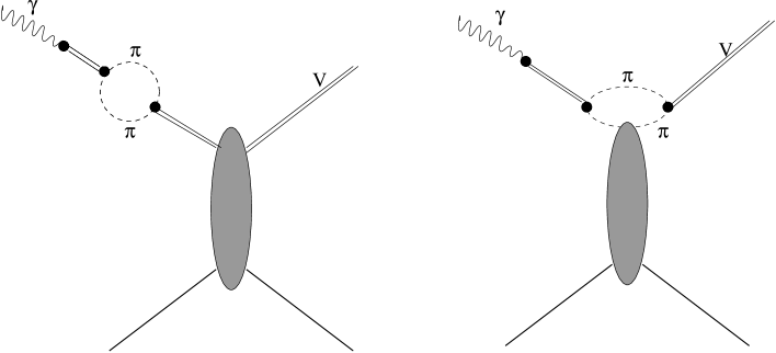
FIG. 2.: Finite width corrections to SVD associated with the $2\pi$- channel. The first diagram is a propagator correction, the second a $2\pi$- scattering contribution.

FIG. 3.: The reduced wave function $\Phi_{\rho}$ calculated at zero impact parameter for lead nuclei at 6.1 GeV. The parameters are those of our final fit(see Table III below.)

FIG. 4.: The profile function $\Gamma_{\rho}$ calculated for lead nuclei at 6.1 GeV. The parameters are those of our final fit(see Table III below).

FIG. 5.: Comparison between different theoretical predictions and the complex nuclei data for $E_{\gamma}$=6.1 GeV: the SVD-prediction assuming the parameter values of Table II (dashed dotted line); the GVD solution in the approximation (28) using the parameter values given by Kroker [24] (dashed line); and the full GVD prediction using the same parameters (solid line) .

FIG. 6.: The optical moddel GVD fit to the complex nuclei data at 6.1 GeV, corresponding to the parameters of Table III.(The deuteron data point shown is not included in the fit for obvious reasons.)

FIG. 7.: The optical model GVD fit to the complex nuclei data at 6.5 GeV, corresponding to the parameters of Table III.(The deuteron data point shown is not included in the fit for obvious reasons.)

FIG. 8.: The optical model GVD fit to the complex nuclei data at 8.8 GeV, corresponding to the parameters of Table III.(The deuteron data point shown is not included in the fit for obvious reasons.)

REFERENCES

- [1] G. Shaw, Phys. Lett. B226 (1989) 125.
- [2] For a review of shadowing and other nuclear effects in structure functions, see M. Arneodo, Phys. Rep. 240 (1994) 301.
- [3] H. Fraas, B. J. Read and D. Schildknecht, Nucl. Phys. B86 (1975) 346; P. Ditsas and G. Shaw, Nucl. Phys. B113 (1976) 346; P. Moseley and G. Shaw, J. Phys. G 21 (1995) 1043.
- [4] S.J.Brodsky, G.Grammer Jr., P.Lepage and J.D.Sullivan(unpublished,1978); this work is descibed by G.Grammer Jr. and J.D.Sullivan in ”Electromagnetic Interactions of Hadrons” vol.2, ed. A.Donnachie and G.Shaw, Plenum Press, New York, 1978. ( Cf. section 2.1.3.)
- [5] The European Muon(EMC) Collaboration, Phys. Lett. B211 (1988) 493.
- [6] G. Shaw, Phys. Rev. D47 (1993) R3676
- [7] D.O.Caldwell et.al., Phys. Rev. Lett. 42, 553 (1979);
- [8] New Muon(NMC) Collaboration, Z.Phys. C51, 387 (1991); Z.Phys. C53, 73 (1992); Fermilab E665 Collaboration, Phys. Rev. Lett. 68, 3266 (1992)
- [9] P. Moseley and G. Shaw, Phys. Rev. D52 (1995) 4941; G. Kerley and G. Shaw Phys. Rev. D56 (1997) (in press).
- [10] H1 collaboration: S. Aid et al. Nucl. Phys. B470 (1996) 3; ZEUS collaboration: M. Derrick et al. Zeit. Phys. C72 (1996) 399; E665 collaboration: M. R. Adams et al. Phys. Rev. D54 (1996) 3006.
- [11] A. Donnachie and P. V. Landshoff, Phys. Lett. 348B (1995) 213
- [12] ZEUS collaboration, Z.Phys. C69 (1995) 39
- [13] H1 collaboration, Nucl.Phys. B463 (1996) 3
- [14] D.W.G.S.Leith, ”High energy photoproduction: diffractive processes” in ‘Electromagnetic Interactions of Hadrons’, Vol. 1, ed. A. Donnachie and G. Shaw (Plenum, New York, 1978)
- [15] H. Alvensleben et al. Nucl. Phys. B18 (1970) 333
- [16] G. McClellan et al. Phys. Rev. D4, (1971) 2683
- [17] Particle data group, Phys. Rev. D54 (1996) 1
- [18] D. Aston et al. Nucl. Phys. B209 (1982) 56
- [19] T.H.Bauer and D.R.Yennie, Phys. Lett. 60B (1976) 169
- [20] For reviews of GVD models, see A.Donnachie and G.Shaw in ‘Electromagnetic Interactions of Hadrons’, Vol. 2, ed.A. Donnachie and G.Shaw (Plenum, New York, 1978); and G. Shaw, Phys. Lett. B318 (1993) 221.
- [21] R.J. Glauber in ”Lectures in Theoretical Physics”, Editors W.E. Brittin, L.G. Dunham, Interscience Publishers, Inc., New York (1959)
- [22] G. Grammer and J.D. Sullivan in ”Electromagnetic Interactions ofHadrons, Vol.2, Plenum Press (1978), Editors A. Donnachie and G. Shaw
- [23] R.D. Spital, D.R. Yennie (1974), Phys. Rev D9, 138.
- [24] M. Kroker (1994), M.Sc. Thesis, Univ. of Manchester.
- [25] A.Donnachie and P.V.Landshoff, Phys. Lett. B296 (1993) 227