hep-ph/9710217
UM-TH-97-25
SLAC-PUB-7668
(revised version)

Three-body decays of selectrons and smuons in

low-energy supersymmetry breaking models

S. Ambrosanio, Graham D. Kribs

Randall Physics Laboratory, University of Michigan,
Ann Arbor, MI 48109–1120

and
Stephen P. Martin

Stanford Linear Accelerator Center, Stanford University,
Stanford, CA 94309

In models with low-energy supersymmetry breaking, it is well-known that charged sleptons can be significantly lighter than the lightest neutralino, with the gravitino and lighter stau being the lightest and next-to-lightest supersymmetric particles respectively. We give analytical formulas for the three-body decays of right-handed selectrons and smuons into final states involving a tau, a stau, and an electron or muon, which are relevant in this scenario. We find that the three-body decays dominate over much of the parameter space, but the two-body decays into a lepton and a gravitino can compete if the three-body phase space is small and the supersymmetry-breaking scale (governing the two-body channel) is fairly low. We study this situation quantitatively for typical gauge-mediated supersymmetry breaking model parameters. The three-body decay lengths are possibly macroscopic, leading to new unusual signals. We also analyze the final-state energy distributions, and briefly assess the prospects for detecting these decays at CERN LEP2 and other colliders.

1. Introduction

Supersymmetry-breaking effects in the Minimal Supersymmetric Standard Model (MSSM) are usually introduced explicitly as soft terms in the lagrangian. In a more complete theory, supersymmetry is expected to be an exact local symmetry of the lagrangian which is spontaneously broken in the vacuum state in a sector of particles distinct from the MSSM. There are two main proposals for how supersymmetry breaking is communicated to the MSSM particles. Historically, the more popular approach has been that supersymmetry breaking occurs at a scale $\mathrel{\>{\hbox{\raise 1.50696pt\hbox{$>$}}\kern-3.8889pt\kern-3.8889pt\hbox{\lower 2.79857pt\hbox{$\sim$}}}\>}10^{10}$ GeV and is communicated to the MSSM dominantly by gravitational interactions. In this case, the lightest supersymmetric particle (LSP) is naturally the lightest neutralino $({\tilde{N}}_{1})$. One of the virtues of this gravity-mediated supersymmetry breaking scenario is that a neutralino LSP can easily have the correct relic density to make up the cold dark matter with a cosmologically acceptable density.

Recently, there has been a resurgence of interest in the idea [1, 2] that supersymmetry-breaking effects are communicated to the MSSM by the ordinary $SU(3)_{C}\times SU(2)_{L}\times U(1)_{Y}$ gauge interactions rather than gravity. This gauge-mediated supersymmetry breaking (GMSB) scenario allows the ultimate supersymmetry-breaking order parameter $\sqrt{F}$ to be much smaller than $10^{10}$ GeV, perhaps even as small as $10^{4}$ GeV or so, with the important implication that the gravitino $(\tilde{G})$ is the LSP. The spin-$3/2$ gravitino absorbs the would-be goldstino of supersymmetry breaking as its longitudinal (helicity $\pm 1/2$) components by the super-Higgs mechanism, obtaining a mass $m_{\tilde{G}}={F/\sqrt{3}M_{P}}=2.37(\sqrt{F}/100\>{\rm TeV})^{2}\>{\rm eV},$ where $M_{P}=(8\pi G_{\rm Newton})^{-1/2}=2.4\times 10^{18}$ GeV is the reduced Planck mass. The gravitino inherits the non-gravitational interactions of the goldstino it has absorbed [3]. This means that the next-to-lightest supersymmetric particle (NLSP) can decay into its standard model partner and a gravitino with a characteristic decay length which can be less than of order 100 microns (for $\sqrt{F}\mathrel{\>{\hbox{\raise 1.50696pt\hbox{$<$}}\kern-3.8889pt\kern-3.8889pt\hbox{\lower 2.79857pt\hbox{$\sim$}}}\>}10^{5}$ GeV) or more than a kilometer (for $\sqrt{F}\mathrel{\>{\hbox{\raise 1.50696pt\hbox{$>$}}\kern-3.8889pt\kern-3.8889pt\hbox{\lower 2.79857pt\hbox{$\sim$}}}\>}10^{7}$ GeV), or anything in between. This leads to many intriguing phenomenological possibilities which are unique to models of low-energy supersymmetry breaking [3-10]. For kinematical purposes, the gravitino is essentially massless. The perhaps surprising relevance of a light gravitino for collider physics can be traced to the fact that the interactions of the longitudinal components of the gravitino are the same as those of the goldstino it has absorbed, and are proportional to $1/m_{\tilde{G}}$ (or equivalently to $1/F$) in the light gravitino (small $F$) limit [3].

In a large class of models with low-energy supersymmetry breaking, the NLSP will either be the lightest neutralino or the lightest stau $({\tilde{\tau}}_{1})$ mass eigenstate. Our convention for the stau mixing angle $\theta_{\tilde{\tau}}$ is such that

$$\pmatrix{{\tilde{\tau}}_{1}\cr{\tilde{\tau}}_{2}}=\pmatrix{\cos\theta_{\tilde{\tau}}&\sin\theta_{\tilde{\tau}}\cr-\sin\theta_{\tilde{\tau}}&\cos\theta_{\tilde{\tau}}}\pmatrix{{\tilde{\tau}}_{L}\cr{\tilde{\tau}}_{R}}$$ (1)

with $m_{\tilde{\tau}_{1}}<m_{\tilde{\tau}_{2}}$ and $0\leq\theta_{{\tilde{\tau}}}<\pi$ (so $\sin\theta_{\tilde{\tau}}\geq 0$). The sign of $\cos\theta_{\tilde{\tau}}$ depends on the sign of $\mu$ (the superpotential Higgs mass parameter) through the off-diagonal term $-\mu m_{\tau}\tan\beta$ in the stau (mass)² matrix. This term typically dominates over the contribution from the soft trilinear scalar couplings in GMSB models, because the latter are very small at the messenger scale and because the effects of renormalization group running are usually not very large. For this reason, it is quite unlikely that cancellation can lead to $\cos\theta_{\tilde{\tau}}\approx 0$ in these models, unless the scale of supersymmetry breaking is quite high. In GMSB models like those in Ref. [9] which are relevant to the decays studied in this paper, $|\cos\theta_{\tilde{\tau}}|$ ranges from about $0.1$ to $0.3$ when the mass splittings between ${\tilde{\tau}}_{1}$ and the lighter selectron and smuon are less than about 10 GeV. That is the situation we will be interested in here. The selectrons and smuons also mix exactly analogously to Eq. (1). However, at least in GMSB models, their mixings are generally much smaller, with $\cos\theta_{\tilde{\mu}}/\cos\theta_{\tilde{\tau}}\sim y_{\mu}/y_{\tau}\approx 0.06$ and $\cos\theta_{\tilde{e}}/\cos\theta_{\tilde{\tau}}\sim y_{e}/y_{\tau}\approx 3\times 10^{-4}$. Therefore, in most cases one can just treat the lighter selectron and smuon mass eigenstates as nearly unmixed and degenerate states. We will write these mass eigenstates as $\tilde{e}_{R}$ and $\tilde{\mu}_{R}$, despite their small mixing. We will also assume, as is the case in minimal GMSB models, that there are no lepton flavor violating couplings or mixings.

The termination of superpartner decay chains depends crucially on the differences between $m_{{\tilde{N}}_{1}}$, $m_{{\tilde{\tau}}_{1}}$, and $m_{\tilde{\ell}_{R}}$ (in this paper $\ell$ is generic notation for $e$ or $\mu$). We assume that $R$-parity violation is absent, so that there are no competing decays for the NLSP. If the NLSP is ${\tilde{N}}_{1}$ with $m_{{\tilde{N}}_{1}}<m_{{\tilde{\tau}}_{1}}-m_{\tau}$, then the decay ${\tilde{N}}_{1}\rightarrow\gamma\tilde{G}$ can lead to new discovery signals for supersymmetry, as explored in Refs. [3-9]. In other models, one finds that the NLSP is ${\tilde{\tau}}_{1}$ [6]. Here one must distinguish between several qualitatively distinct scenarios. If $\tan\beta$ is not too large, then ${\tilde{e}}_{R}$ and ${\tilde{\mu}}_{R}$ will not be much heavier than ${\tilde{\tau}}_{1}$, and the decays ${\tilde{\ell}}_{R}\rightarrow\ell\tau{\tilde{\tau}}_{1}$ and ${\tilde{\ell}}_{R}\rightarrow\ell{\tilde{N}}_{1}$ will not be kinematically open. In this “slepton co-NLSP scenario”, each of ${\tilde{e}}_{R}$, ${\tilde{\mu}}_{R}$, and ${\tilde{\tau}}_{1}$ may decay according to ${\tilde{e}}_{R}\rightarrow e\tilde{G}$, ${\tilde{\mu}}_{R}\rightarrow\mu\tilde{G}$ and ${\tilde{\tau}}_{1}\rightarrow\tau\tilde{G}$, possibly with very long lifetimes. There can also be competing three-body decays ${\tilde{\ell}}_{R}\rightarrow\nu_{\ell}\overline{\nu}_{\tau}{\tilde{\tau}}_{1}$ through off-shell charginos ($\tilde{C}_{i}$). However, these decays are strongly suppressed by phase space and because the coupling of ${\tilde{\ell}}_{R}$ to $\nu_{\ell}\tilde{C}_{i}$ is very small. In the approximations that $m_{{\tilde{\ell}}_{R}}^{2}-m_{{\tilde{\tau}}_{1}}^{2}\ll m_{{\tilde{C}}_{1}}^{2}$ and $1-m^{2}_{{\tilde{\tau}}_{1}}/m^{2}_{{\tilde{\ell}}_{R}}\ll 1$, one finds

$$\Gamma({\tilde{\ell}}_{R}^{-}\rightarrow\nu_{\ell}\overline{\nu}_{\tau}{\tilde{\tau}}^{-}_{1})={\alpha^{2}m_{{\tilde{\ell}}_{R}}\over 960\pi\sin^{4}\theta_{W}}\left(1-{m_{{\tilde{\tau}}_{1}}^{2}\over m_{{\tilde{\ell}}_{R}}^{2}}\right)^{5}\sum_{i,j=1,2}{d_{i}^{\tilde{\ell}*}d_{j}^{\tilde{\ell}}d_{i}^{\tilde{\tau}}d_{j}^{\tilde{\tau}*}\over(m^{2}_{\tilde{C}_{i}}/m_{{\tilde{\ell}}_{R}}^{2}-1)(m^{2}_{\tilde{C}_{j}}/m_{{\tilde{\ell}}_{R}}^{2}-1)}$$ (2)

where $d_{i}^{\tilde{f}}=U_{i1}\cos\theta_{\tilde{f}}-(y_{f}/g)U_{i2}\sin\theta_{\tilde{f}}$, with Yukawa couplings $y_{f}=gm_{f}/(\sqrt{2}m_{W}\cos\beta)$, for $f=\ell,\tau$. Here $U_{ij}$ is one of the chargino mixing matrices in the notation of [11] and $g$ is the $SU(2)_{L}$ gauge coupling. (Of course, the decay ${\tilde{\ell}}_{R}^{+}\rightarrow\overline{\nu}_{\ell}\nu_{\tau}{\tilde{\tau}}^{+}_{1}$ has the same width.) For ${\tilde{\mu}}_{R}$ decays, we find that this width is always less than about $10^{-7}$ eV in GMSB models like the ones discussed in [9] if $m_{{\tilde{\mu}}_{R}}-m_{{\tilde{\tau}}_{1}}<m_{\tau}$ and $m_{\tilde{\mu}_{R}}\mathrel{\>{\hbox{\raise 1.50696pt\hbox{$>$}}\kern-3.8889pt\kern-3.8889pt\hbox{\lower 2.79857pt\hbox{$\sim$}}}\>}80$ GeV. The maximum width decreases with increasing $m_{\tilde{\mu}_{R}}$ as long as we continue to require that the decay $\tilde{\mu}_{R}\rightarrow\mu\tau{\tilde{\tau}}_{1}$ is not kinematically open. (For the corresponding ${\tilde{e}}_{R}$ decays, the width is more than four orders of magnitude smaller.) This corresponds to physical decay lengths of (at least) a few meters unless the sleptons are produced very close to threshold. It is possible to have somewhat enhanced widths if $m_{{\tilde{C}}_{1}}-m_{{\tilde{\tau}}_{1}}$ is decreased or if $\cos\theta_{\tilde{\mu}}$ is increased compared to the values typically found in GMSB models. However, even if the decays ${\tilde{\ell}}_{R}\rightarrow\nu_{\ell}\overline{\nu}_{\tau}{\tilde{\tau}}_{1}$ can occur within a detector, they will be extraordinarily hard to detect because the neutrinos are unobserved and the ${\tilde{\tau}}_{1}$ momentum in the lab frame will not be very different from that of the decaying ${\tilde{\ell}}_{R}$. The subsequent decays ${\tilde{\tau}}_{1}\rightarrow\tau\tilde{G}$ can be distinguished from the direct ${\tilde{\ell}}_{R}\rightarrow\ell\tilde{G}$, but if the latter can occur within the detector, then they will likely dominate over ${\tilde{\ell}}_{R}\rightarrow\nu_{\ell}\overline{\nu}_{\tau}{\tilde{\tau}}_{1}$ anyway. So it is very doubtful that the decays ${\tilde{\ell}}_{R}\rightarrow\nu_{\ell}\overline{\nu}_{\tau}{\tilde{\tau}}_{1}$ can play a role in collider phenomenology.

For larger values of $\tan\beta$, enhanced stau mixing renders $\tilde{\tau}_{1}$ lighter than ${\tilde{e}}_{R}$ and ${\tilde{\mu}}_{R}$ by more than $m_{\tau}$. In this “stau NLSP scenario”, all supersymmetric decay chains should (naively) terminate in ${\tilde{\tau}}_{1}\rightarrow\tau\tilde{G}$ [6, 10, 9], again possibly with a very long lifetime. If the mass ordering is $m_{{\tilde{\mu}}_{R}}-m_{\mu}$ and/or $m_{{\tilde{e}}_{R}}-m_{e}>m_{{\tilde{N}}_{1}}$, then the two-body decays ${\tilde{\mu}}_{R}\rightarrow\mu{\tilde{N}}_{1}$ and/or ${\tilde{e}}_{R}\rightarrow e{\tilde{N}}_{1}$ will be open and will dominate. In the rest of this paper, we will instead consider the situation in the stau NLSP scenario in which $m_{{\tilde{N}}_{1}}>m_{{\tilde{\ell}}_{R}}-m_{\ell}>m_{{\tilde{\tau}}_{1}}+m_{\tau}$. In that case, ${\tilde{\mu}}_{R}$ and/or ${\tilde{e}}_{R}$ can decay through off-shell neutralinos in three-body modes ${\tilde{\mu}}_{R}\rightarrow\mu\tau{\tilde{\tau}}_{1}$ and/or ${\tilde{e}}_{R}\rightarrow e\tau{\tilde{\tau}}_{1}$, as shown in Fig. 1.

Figure 1: Right-handed selectrons and smuons can decay according to ${\tilde{\ell}}_{R}^{-}\rightarrow\ell^{-}\tau^{+}{\tilde{\tau}}_{1}^{-}$ or ${\tilde{\ell}}_{R}^{-}\rightarrow\ell^{-}\tau^{-}{\tilde{\tau}}_{1}^{+}$, with different matrix elements, through virtual neutralinos ${\tilde{N}}_{i}$ ($i=1,2,3,4$).

Here one must be careful to distinguish between the different charge channels $\tau^{+}{\tilde{\tau}}_{1}^{-}$ and $\tau^{-}{\tilde{\tau}}_{1}^{+}$ in the final state, for a given charge of the decaying slepton. In the following we will give formulas for $\Gamma({\tilde{\ell}}_{R}^{-}\rightarrow\ell^{-}\tau^{+}{\tilde{\tau}}_{1}^{-})$ and $\Gamma({\tilde{\ell}}_{R}^{-}\rightarrow\ell^{-}\tau^{-}{\tilde{\tau}}_{1}^{+})$, which in general can be quite different, except when the virtual neutralino is nearly on shell. [Of course, these are equal to $\Gamma({\tilde{\ell}}_{R}^{+}\rightarrow\ell^{+}\tau^{-}{\tilde{\tau}}_{1}^{+})$ and $\Gamma({\tilde{\ell}}_{R}^{+}\rightarrow\ell^{+}\tau^{+}{\tilde{\tau}}_{1}^{-})$, respectively.] These three-body slepton decays have been rightly ignored in previous phenomenological discussions of the MSSM with a neutralino LSP, in which the two-body decays ${\tilde{\ell}}_{R}\rightarrow\ell{\tilde{N}}_{1}$ (and possibly others) are always open. However, in models with a gravitino LSP, ${\tilde{N}}_{1}$ is allowed to be much heavier, so it is important to realize that three-body decays of ${\tilde{e}}_{R}$ and ${\tilde{\mu}}_{R}$ are relevant and can in principle imply long lifetimes and macroscopic decay lengths. In the following, we will present analytical results for the three-body decay widths of ${\tilde{e}}_{R}$ and ${\tilde{\mu}}_{R}$, and study numerical results for typical relevant model parameters.

2. Three-body slepton decay widths

Let us first consider the “slepton-charge preserving” decay ${\tilde{\ell}}_{R}^{-}\rightarrow\ell^{-}\tau^{+}{\tilde{\tau}}_{1}^{-}$, keeping ${\tilde{\ell}}$ mixing effects. The matrix element for the relevant Feynman diagrams in Fig. 1 can be written as

$${\cal M}=\sum_{j=1}^{4}{\overline{u}}(p_{\ell})(P_{R}a_{j}^{\tilde{\ell}*}+P_{L}b_{j}^{\tilde{\ell}*}){\hbox to0.0pt{\hbox to5.03125pt{\hfil/\hfil}\hss}p_{\ell}-\hbox to0.0pt{\hbox to5.03125pt{\hfil/\hfil}\hss}p_{{\tilde{\ell}}_{R}}+m_{{\tilde{N}}_{j}}\over[m_{{\tilde{N}}_{j}}^{2}-m_{{\tilde{\ell}}_{R}}^{2}(1-x_{\ell}+r_{\ell}^{2})]}(P_{L}a_{j}^{\tilde{\tau}}+P_{R}b_{j}^{\tilde{\tau}})v(p_{\tau}),$$ (3)

where $P_{L,R}=(1\pm\gamma_{5})/2$, and $x_{\ell}=2p_{{\tilde{\ell}}_{R}}\cdot p_{\ell}/p^{2}_{{\tilde{\ell}}_{R}}$, and

$$a^{\tilde{\tau}}_{j} = \sqrt{2}g^{\prime}N_{j1}\sin\theta_{{\tilde{\tau}}}+y_{\tau}N_{j3}\cos\theta_{{\tilde{\tau}}};$$ (4)

$$b_{j}^{\tilde{\tau}} = -{1\over\sqrt{2}}(g^{\prime}N^{*}_{j1}+gN_{j2}^{*})\cos\theta_{{\tilde{\tau}}}+y_{\tau}N^{*}_{j3}\sin\theta_{{\tilde{\tau}}},$$ (5)

with exactly analogous formulas for $a_{j}^{\tilde{\ell}}$ and $b_{j}^{\tilde{\ell}}$, with $\tilde{\tau}\rightarrow\tilde{\ell}$. Here we have adopted the notation of Ref. [11] for the unitary (complex) neutralino mixing matrix $N_{ij}$ with all $m_{\tilde{N}_{i}}$ real and positive, and $g$ and $g^{\prime}$ are the $SU(2)_{L}$ and $U(1)_{Y}$ gauge couplings. Our fermion propagator is proportional to $(-\hbox to0.0pt{\hbox to5.03125pt{\hfil/\hfil}\hss}p+m)/(p^{2}+m^{2})$, with a spacetime metric signature $(-\mbox{+++})$.

Summing over final state spins and performing the phase space integration, we obtain:

$$\Gamma({\tilde{\ell}}_{R}^{-}\rightarrow\ell^{-}\tau^{+}{\tilde{\tau}}^{-}_{1})={m_{{\tilde{\ell}}_{R}}\over 512\pi^{3}}\sum_{i,j=1}^{4}\sum_{a=1}^{6}c^{(a)}_{ij}I^{(a)}_{ij}$$ (6)

in terms of coefficients

$$c^{(1)}_{ij}=a_{j}^{{\tilde{\ell}}*}a_{j}^{\tilde{\tau}}a_{i}^{{\tilde{\ell}}}a_{i}^{{\tilde{\tau}}*}+b_{j}^{{\tilde{\ell}}*}b_{j}^{\tilde{\tau}}b_{i}^{{\tilde{\ell}}}b_{i}^{{\tilde{\tau}}*},$$ (7)

$$c^{(2)}_{ij}=a_{j}^{{\tilde{\ell}}*}b_{j}^{\tilde{\tau}}a_{i}^{{\tilde{\ell}}}b_{i}^{{\tilde{\tau}}*}+b_{j}^{{\tilde{\ell}}*}a_{j}^{\tilde{\tau}}b_{i}^{{\tilde{\ell}}}a_{i}^{{\tilde{\tau}}*},$$ (8)

$$c^{(3)}_{ij}=2{\rm Re}[a_{j}^{{\tilde{\ell}}*}b_{j}^{\tilde{\tau}}a_{i}^{{\tilde{\ell}}}a_{i}^{{\tilde{\tau}}*}+b_{j}^{{\tilde{\ell}}*}a_{j}^{\tilde{\tau}}b_{i}^{{\tilde{\ell}}}b_{i}^{{\tilde{\tau}}*}],$$ (9)

$$c^{(4)}_{ij}=-2{\rm Re}[a_{j}^{{\tilde{\ell}}*}b_{j}^{\tilde{\tau}}b_{i}^{{\tilde{\ell}}}b_{i}^{{\tilde{\tau}}*}+b_{j}^{{\tilde{\ell}}*}a_{j}^{\tilde{\tau}}a_{i}^{{\tilde{\ell}}}a_{i}^{{\tilde{\tau}}*}],$$ (10)

$$c^{(5)}_{ij}=-4{\rm Re}[b_{j}^{{\tilde{\ell}}*}a_{j}^{\tilde{\tau}}a_{i}^{{\tilde{\ell}}}b_{i}^{{\tilde{\tau}}*}],$$ (11)

$$c^{(6)}_{ij}=-4{\rm Re}[a_{j}^{{\tilde{\ell}}*}a_{j}^{\tilde{\tau}}b_{i}^{{\tilde{\ell}}}b_{i}^{{\tilde{\tau}}*}],$$ (12)

and dimensionless integrals $I_{ij}^{(a)}$ defined as follows. First, we introduce the mass ratios $r_{{\tilde{\tau}}}=m_{{\tilde{\tau}}_{1}}/m_{{\tilde{\ell}}_{R}}$, $r_{\tau}=m_{\tau}/m_{{\tilde{\ell}}_{R}}$, $r_{\ell}=m_{\ell}/m_{{\tilde{\ell}}_{R}}$, and $r_{{\tilde{N}}_{i}}=m_{{\tilde{N}}_{i}}/m_{{\tilde{\ell}}_{R}}$ with $r_{\ell}\ll r_{\tau}\ll r_{{\tilde{\tau}}}<1-r_{\tau}-r_{\ell}$ and $r_{{\tilde{N}}_{1}}>1-r_{\ell}$. Then we find

$$I_{ij}^{(1)} = \int dx_{\ell}\>\,(x_{\ell}-2r_{\ell}^{2})(1-x_{\ell}+r_{\ell}^{2})(1-x_{\ell}+r_{\ell}^{2}+r_{\tau}^{2}-r_{{\tilde{\tau}}}^{2})f_{ij},$$ (13)

$$I_{ij}^{(2)} = r_{{\tilde{N}}_{i}}r_{{\tilde{N}}_{j}}\int dx_{\ell}\>\,(x_{\ell}-2r_{\ell}^{2})(1-x_{\ell}+r_{\ell}^{2}+r_{\tau}^{2}-r_{{\tilde{\tau}}}^{2})f_{ij},$$ (14)

$$I_{ij}^{(3)} = 2r_{\tau}r_{{\tilde{N}}_{j}}\int dx_{\ell}\>\,(x_{\ell}-2r_{\ell}^{2})(1-x_{\ell}+r_{\ell}^{2})f_{ij},$$ (15)

$$I_{ij}^{(4)} = 2r_{\ell}r_{{\tilde{N}}_{j}}\int dx_{\ell}\>\,(1-x_{\ell}+r_{\ell}^{2})(1-x_{\ell}+r_{\ell}^{2}+r_{\tau}^{2}-r_{{\tilde{\tau}}}^{2})f_{ij},$$ (16)

$$I_{ij}^{(5)} = 2r_{\ell}r_{\tau}r_{\tilde{N}_{i}}r_{\tilde{N}_{j}}\int dx_{\ell}\>\,(1-x_{\ell}+r_{\ell}^{2})f_{ij},$$ (17)

$$I_{ij}^{(6)} = 2r_{\ell}r_{\tau}\int dx_{\ell}\>\,(1-x_{\ell}+r_{\ell}^{2})^{2}f_{ij},$$ (18)

where

$$f_{ij}={\sqrt{x_{\ell}^{2}-4r_{\ell}^{2}}\>\lambda^{1/2}[1-x_{\ell}+r_{\ell}^{2},r_{\tau}^{2},r_{{\tilde{\tau}}}^{2}]\over(1-x_{\ell}+r_{\ell}^{2})^{2}\,(r_{{\tilde{N}}_{i}}^{2}-1+x_{\ell}-r_{\ell}^{2})\,(r_{{\tilde{N}}_{j}}^{2}-1+x_{\ell}-r_{\ell}^{2})}$$ (19)

with $\lambda^{1/2}[a,b,c]=\sqrt{a^{2}+b^{2}+c^{2}-2ab-2ac-2bc}$. The limits of integration for $x_{\ell}$ are $2r_{\ell}<x_{\ell}<1+r_{\ell}^{2}-r_{\tau}^{2}-r_{{\tilde{\tau}}}^{2}-2r_{\tau}r_{{\tilde{\tau}}}$. The matrix element and decay width for the “slepton-charge flipping” channel ${\tilde{\ell}}_{R}^{-}\rightarrow\ell^{-}\tau^{-}{\tilde{\tau}}_{1}^{+}$ are obtained by replacing $a_{j}^{\tilde{\tau}}\rightarrow b_{j}^{\tilde{\tau}*}$ and $b_{j}^{\tilde{\tau}}\rightarrow a_{j}^{\tilde{\tau}*}$ everywhere in the above equations.

In GMSB models like those studied in Ref. [9] which are relevant to these decays, one finds that $m_{{\tilde{e}}_{R}}-m_{{\tilde{\mu}}_{R}}$ is at the most a few tens of MeV, so we will neglect the distinction between $m_{{\tilde{e}}_{R}}$ and $m_{{\tilde{\mu}}_{R}}$. It is an excellent approximation to take $r_{\mu}=0$ except when the mass difference

$$\Delta m=m_{{\tilde{\ell}}_{R}}-m_{{\tilde{\tau}}_{1}}-m_{\tau}$$ (20)

is a few hundred MeV or less, and $r_{e}=0$ is of course nearly always a good approximation. It is also generally an excellent approximation to neglect smuon and selectron mixing and Yukawa couplings in the matrix element, so that $a_{j}^{\tilde{\ell}}\approx\sqrt{2}g^{\prime}N_{j1}$ and $b_{j}^{\tilde{\ell}}\approx 0$. The effects of $I_{ij}^{(4,5,6)}$ are usually quite negligible because of the $r_{\ell}$ and $b_{j}^{{\tilde{\ell}}}$ suppressions. An instructive limit which is often approximately realized in GMSB models (or, in generic models with gaugino mass unification, whenever $|\mu|$ is sizeably larger than the gaugino mass parameters) is the case in which the contributions from a Bino-like ${\tilde{N}}_{1}$ dominate, with $m_{{\tilde{N}}_{1}}\approx 0.5m_{{\tilde{N}}_{2}}\ll m_{{\tilde{N}}_{3}},m_{{\tilde{N}}_{4}}$. Since the decaying ${\tilde{\ell}}_{R}$ essentially couples only to the Bino ($\tilde{B}$) component of the virtual neutralinos, this approximation is quite good for a large class of models where $|N_{11}|$ is not too far from 1. In that case, we may neglect the contributions of virtual $\tilde{N}_{2}$, $\tilde{N}_{3}$ and $\tilde{N}_{4}$ because of the coupling constant suppressions together with the suppressions due to larger neutralino masses. With these approximations, the expressions for the decay widths simplify to

$$\Gamma({\tilde{\ell}}_{R}^{-}\rightarrow\ell^{-}\tau^{+}{\tilde{\tau}}^{-}_{1})\approx{m_{{\tilde{\ell}}_{R}}\over 512\pi^{3}}\left[|A_{1}|^{2}I_{11}^{(1)}+|B_{1}|^{2}I_{11}^{(2)}-2{\rm Re}(A_{1}B_{1}^{*})\,I_{11}^{(3)}\right],$$ (21)

$$A_{1}=2g^{\prime 2}|N_{11}|^{2}\sin\theta_{\tilde{\tau}}+\sqrt{2}g^{\prime}y_{\tau}N_{11}^{*}N_{13}\cos\theta_{{\tilde{\tau}}},$$ (22)

$$B_{1}=g^{\prime 2}N_{11}^{*2}\cos\theta_{\tilde{\tau}}+gg^{\prime}N^{*}_{11}N_{12}^{*}\cos\theta_{{\tilde{\tau}}}-\sqrt{2}g^{\prime}y_{\tau}N^{*}_{11}N^{*}_{13}\sin\theta_{\tilde{\tau}},$$ (23)

and

$$\Gamma({\tilde{\ell}}_{R}^{-}\rightarrow\ell^{-}\tau^{-}{\tilde{\tau}}^{+}_{1})\approx{m_{{\tilde{\ell}}_{R}}\over 512\pi^{3}}\left[|B^{\prime}_{1}|^{2}I_{11}^{(1)}+|A^{\prime}_{1}|^{2}I_{11}^{(2)}-2{\rm Re}(A^{\prime}_{1}B_{1}^{\prime*})\,I_{11}^{(3)}\right],$$ (24)

$$A^{\prime}_{1}=2g^{\prime 2}N_{11}^{2}\sin\theta_{\tilde{\tau}}+\sqrt{2}g^{\prime}y_{\tau}N_{11}N_{13}\cos\theta_{{\tilde{\tau}}},$$ (25)

$$B^{\prime}_{1}=g^{\prime 2}|N_{11}|^{2}\cos\theta_{\tilde{\tau}}+gg^{\prime}N_{11}N_{12}^{*}\cos\theta_{{\tilde{\tau}}}-\sqrt{2}g^{\prime}y_{\tau}N_{11}N^{*}_{13}\sin\theta_{\tilde{\tau}}.$$ (26)

We will be interested in the situation in which $\Delta m$ is small (less than 10 GeV). This implies that $\tan\beta$ is not too large, and thus ${\tilde{\tau}}_{1}$ has a large ${\tilde{\tau}}_{R}$ content. However, as we will see in the next section, it is usually not a good approximation to neglect stau mixing altogether (by setting $\sin\theta_{{\tilde{\tau}}}=1$, $\cos\theta_{{\tilde{\tau}}}=0$ everywhere), because $|\cos\theta_{{\tilde{\tau}}}|$ is likely to be at least $0.1$ as we have already mentioned. Near threshold, the range of integration includes only small values of $x_{\ell}$, so that the dimensionless integrals $I_{11}^{(1)}$ and $I_{11}^{(2)}$ and $I_{11}^{(3)}$ scale approximately proportional to $1/(r_{{\tilde{N}}_{1}}^{2}-1)^{2}$ and $r^{2}_{{\tilde{N}}_{1}}/(r_{{\tilde{N}}_{1}}^{2}-1)^{2}$ and $r_{{\tilde{N}}_{1}}/(r_{{\tilde{N}}_{1}}^{2}-1)^{2}$, respectively. This means that the decay width is suppressed as $r_{{\tilde{N}}_{1}}$ (or equivalently $m_{{\tilde{N}}_{1}}$) is increased, with other parameters held fixed. This is particularly likely in GMSB models with a large messenger sector and a high scale of supersymmetry breaking. Furthermore, the relative sizes of the $I^{(2)}_{11}$ and $I^{(3)}_{11}$ contributions are enhanced in the large $r_{{\tilde{N}}_{1}}$ limit. It is important to note that as $r_{{\tilde{N}}_{1}}$ is increased, $\Gamma({\tilde{\ell}}_{R}^{-}\rightarrow\ell^{-}\tau^{-}{\tilde{\tau}}_{1}^{+})$ becomes larger than $\Gamma({\tilde{\ell}}_{R}^{-}\rightarrow\ell^{-}\tau^{+}{\tilde{\tau}}_{1}^{-})$, because of this effect together with the fact that $A_{1}$ and $A_{1}^{\prime}$ typically have larger magnitudes than $B_{1}$ and $B_{1}^{\prime}$. Note also that the $I^{(3)}_{11}$ contributions appear to be suppressed by a factor of $r_{\tau}$, but this turns out to be illusory since near threshold $m_{\tau}$ is not the only small mass scale in the problem; in particular it can be comparable to or even much larger than $\Delta m-m_{\ell}$ which determines the kinematic suppression of the decay.

3. Numerical results

Some typical results are shown in Figs. 2-5. In Fig. 2,

Figure 2: The decay widths in meV for ${\tilde{e}}_{R}\rightarrow e\tau{\tilde{\tau}}_{1}$ (solid lines) and ${\tilde{\mu}}_{R}\rightarrow\mu\tau{\tilde{\tau}}_{1}$ (dashed lines), including both $\tau^{+}{\tilde{\tau}}^{-}_{1}$ and $\tau^{-}{\tilde{\tau}}^{+}_{1}$ final states, as functions of $\Delta m=m_{{\tilde{\ell}}_{R}}-m_{{\tilde{\tau}}_{1}}-m_{\tau}$. The widths have been computed using Eqs. (21)-(26) with $m_{{\tilde{\ell}}_{R}}=90$ GeV, $\cos\theta_{\tilde{\tau}}=0.15$ and $r_{{\tilde{N}}_{1}}=1.1$, 1.5, 2.0, and 3.0 (from top to bottom), with the approximation $N_{11}=1$ and $N_{12}=N_{13}=0$.

we give the total three-body decay widths for ${\tilde{e}}_{R}$ and ${\tilde{\mu}}_{R}$ (including both $\tau^{+}{\tilde{\tau}}^{-}_{1}$ and $\tau^{-}{\tilde{\tau}}^{+}_{1}$ final states) as functions of $\Delta m$ for $m_{{\tilde{\ell}}_{R}}=90$ GeV and four choices $r_{{\tilde{N}}_{1}}=1.1$, 1.5, 2.0, and 3.0. (In the GMSB models studied in Ref. [9], one finds $r_{{\tilde{N}}_{1}}\mathrel{\>{\hbox{\raise 1.50696pt\hbox{$<$}}\kern-3.8889pt\kern-3.8889pt\hbox{\lower 2.79857pt\hbox{$\sim$}}}\>}1.8$, but it is possible to imagine more general models with larger values.) Here we have chosen the approximation of Eqs. (21)-(26) with $N_{11}=1$ and $\cos\theta_{{\tilde{\tau}}}=0.15$. We use $m_{\tau}=1.777$ GeV, $m_{\mu}=0.1057$ GeV, $\alpha=1/128.0$, and $\sin^{2}\theta_{W}=0.2315$. Realistic model parameters can introduce a significant variation in the decay widths, and in general one should use the full formulas given above for any specific model. Our choice of a positive value for $\cos\theta_{\tilde{\tau}}$ in this example leads to a suppression in the width compared to the opposite choice, because of the sign of the interference terms proportional to $I_{11}^{(3)}$ in Eqs. (21) and (24). These interference terms are often of the order of tens of percent of the total width, showing the importance of keeping the stau mixing effects if real accuracy is needed.

The important ratio of the partial widths for the two charge channels $\Gamma({\tilde{\ell}}_{R}^{-}\rightarrow\ell^{-}\tau^{-}{\tilde{\tau}}_{1}^{+})/\Gamma({\tilde{\ell}}_{R}^{-}\rightarrow\ell^{-}\tau^{+}{\tilde{\tau}}_{1}^{-})$ is shown in Fig. 3 for the case $\ell=e$, as a function of $r_{{\tilde{N}}_{1}}$. Here we have chosen values of $\cos\theta_{{\tilde{\tau}}}=-0.3$, $-0.1$, $0.1$ and $0.3$, and other parameters as in Fig. 2. As expected, this ratio is close to 1 when the virtual neutralino is nearly on-shell, and increases with $r_{{\tilde{N}}_{1}}$. It scales roughly like $I^{(2)}_{11}/I^{(1)}_{11}\approx r_{{\tilde{N}}_{1}}^{2}$, up to significant corrections from the interference term(s). This increase tends to be more pronounced for larger $\cos\theta_{{\tilde{\tau}}}$ in these models.

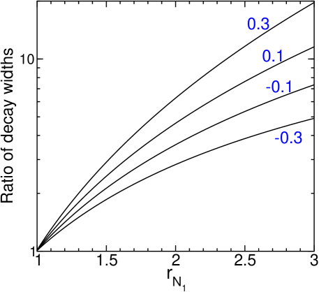
Figure 3: The ratio $\Gamma(\tilde{e}_{R}^{-}\rightarrow e^{-}\tau^{-}{\tilde{\tau}}_{1}^{+})/\Gamma(\tilde{e}_{R}^{-}\rightarrow e^{-}\tau^{+}{\tilde{\tau}}_{1}^{-})$ is shown as a function of $r_{{\tilde{N}}_{1}}$, for four values of $\cos\theta_{{\tilde{\tau}}}=$ $0.3$, $0.1$, $-0.1$ and $-0.3$ (from top to bottom). The widths have been computed using Eqs. (21)-(26) with $m_{\tilde{e}_{R}}=90$ GeV, and with the approximation $N_{11}=1$ and $N_{12}=N_{13}=0$.

Because large $r_{{\tilde{N}}_{1}}$ also corresponds to longer lifetimes, the decay ${\tilde{\ell}}_{R}^{-}\rightarrow\ell^{-}\tau^{-}{\tilde{\tau}}_{1}^{+}$ is likely to dominate if the three-body decay lengths are macroscopic.

The variation with the stau mixing angle is further illustrated in Fig. 4,

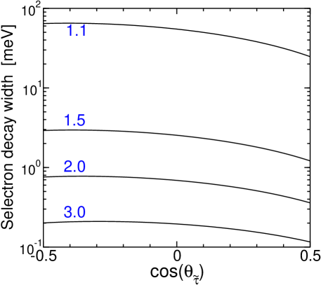
Figure 4: The dependence of $\Gamma({\tilde{e}}_{R}\rightarrow e\tau{\tilde{\tau}}_{1})$ (including both charge final states) on $\cos\theta_{{\tilde{\tau}}}$, computed as in Fig. 2 but with $\Delta m=m_{{\tilde{e}}_{R}}-m_{{\tilde{\tau}}}-m_{\tau}$ held fixed at 1.0 GeV. The four curves correspond to $r_{{\tilde{N}}_{1}}=1.1$, 1.5, 2.0, and 3.0 (from top to bottom).

where we show the total three-body decay width $\Gamma({\tilde{e}}_{R}\rightarrow e\tau{\tilde{\tau}}_{1})$ including both charge final states with $m_{{\tilde{e}}_{R}}=90$ GeV and $\Delta m=1.0$ GeV, $r_{{\tilde{N}}_{1}}=1.1$, 1.5, 2.0, 3.0, for the range $-0.5<\cos\theta_{{\tilde{\tau}}}<0.5$. Note that the total width can vary by a factor of two or more over this range. Here it should be kept in mind that at least in the GMSB models studied in Ref. [9], one finds $0.1\mathrel{\>{\hbox{\raise 1.50696pt\hbox{$<$}}\kern-3.8889pt\kern-3.8889pt\hbox{\lower 2.79857pt\hbox{$\sim$}}}\>}|\cos\theta_{\tilde{\tau}}|\mathrel{\>{\hbox{\raise 1.50696pt\hbox{$<$}}\kern-3.8889pt\kern-3.8889pt\hbox{\lower 2.79857pt\hbox{$\sim$}}}\>}0.3$, so that the whole range shown may not be relevant. In Fig. 5, we show contours of constant total three-body decay widths $\Gamma({\tilde{e}}_{R}\rightarrow e\tau{\tilde{\tau}}_{1})$ in the $\Delta m$ vs. $m_{{\tilde{e}}_{R}}$ plane, for the choice $r_{{\tilde{N}}_{1}}=1.5$ and $\cos\theta_{\tilde{\tau}}=0.15$.

Figure 5: Contours of constant total decay width $\Gamma({\tilde{e}}_{R}\rightarrow e\tau{\tilde{\tau}}_{1})$ (from left to right, 0.0001, 0.001, 0.01, 0.1, 1, 10, 100 and 1000 meV), including both charge channels for the final state, and computed with $r_{{\tilde{N}}_{1}}=1.5$ and $\cos\theta_{\tilde{\tau}}=0.15$ with the same approximations as in Figs. 2-4.

In both figures we continue to use $N_{11}=1$, $N_{12}=N_{13}=0$ in Eqs. (21)-(26). However, it should be emphasized that in realistic models the effects of deviations from this simplistic approximation can be quite appreciable, especially since $|N_{11}|^{2}$ can easily be of order 0.7 or somewhat less in GMSB models, and the width scales essentially like $|N_{11}|^{4}$.

As can be seen from these figures, the physical three-body decay lengths for ${\tilde{e}}_{R}$ and ${\tilde{\mu}}_{R}$ can be quite large if $\Delta m$ is less than a few GeV and/or $m_{{\tilde{N}}_{1}}/m_{{\tilde{\ell}}_{R}}$ is large. In the lab frame, the probability that a slepton ${\tilde{\ell}}_{R}$ with energy $E$ will travel a distance $x$ before decaying is $P(x)=e^{-x/L}$, where

$$L=0.2\left({\Gamma\over 1\>{\rm meV}}\right)^{-1}\Bigl{(}{E^{2}\over m^{2}_{{\tilde{\ell}}_{R}}}-1\Bigr{)}^{1/2}{\rm mm}.$$ (27)

For sleptons pair-produced at LEP2 (or at a next-generation lepton collider), $E$ in Eq. (27) is simply the beam energy. So if $\Delta m$ is less than a GeV or so (depending on $r_{{\tilde{N}}_{1}}$ and the specific couplings of the model), ${\tilde{e}}_{R}$ and ${\tilde{\mu}}_{R}$ could have a macroscopic and measurable decay length. If $\Delta m$ is of order 100 MeV or less, the decay length could even exceed the dimensions of typical detectors.

It is also important to realize that the dominant decay for ${\tilde{\ell}}_{R}$ is not a priori known, since the three-body decays ${\tilde{\ell}}_{R}\rightarrow\ell\tau{\tilde{\tau}}_{1}$ have to compete with the two-body decays to the gravitino ${\tilde{\ell}}_{R}\rightarrow\ell\tilde{G}$. The latter have a width given by

$$\Gamma({\tilde{\ell}}_{R}\rightarrow\ell\tilde{G})={m_{{\tilde{\ell}}_{R}}^{5}/16\pi F^{2}}.$$ (28)

For a given set of weak-scale MSSM parameters leading to a calculable three-body width for ${\tilde{\ell}}_{R}$, the two-body width Eq. (28) is essentially an independent parameter, depending on $\sqrt{F}$ (or on the gravitino mass in “no-scale” supergravity models [13]). For example, for the sets of parameters and corresponding widths in Fig. 2, the three-body decay dominates for $\sqrt{F}\mathrel{\>{\hbox{\raise 1.50696pt\hbox{$>$}}\kern-3.8889pt\kern-3.8889pt\hbox{\lower 2.79857pt\hbox{$\sim$}}}\>}10^{3}$ TeV for $\Delta m-m_{\ell}$ down to a few hundred MeV. Alternatively, the minimum possible value of $\sqrt{F}$ of order 10 TeV in GMSB models corresponds to a maximum width for ${\tilde{\ell}}_{R}\rightarrow\ell\tilde{G}$ of order 20 eV (for $m_{{\tilde{\ell}}_{R}}$ of order 100 GeV), so $\Delta m$ is expected to be larger than of order 10 GeV before the three-body decay dominates. In many of the GMSB models that have actually been constructed including the supersymmetry-breaking sector [2, 12], this limit is not saturated and $\sqrt{F}$ is orders of magnitude larger than 10 TeV, so the three-body decay is expected to dominate unless the mass difference is correspondingly smaller. Conversely, in “no-scale” models, the two-body decay width might even be much larger than the tens of eV range.

4. Energy distributions

If the three-body decays of ${\tilde{e}}_{R}$ and ${\tilde{\mu}}_{R}$ indeed dominate, then the $\ell$ and $\tau$ emitted in the decay can be quite soft if $\Delta m$ is small. Hence, it is important to address the lepton detectability and, in general, the ability to recognize a three-body decay pattern in a real experimental environment. Using CompHEP 3.2 [15] plus an implementation of the MSSM lagrangian [16], we have examined the (s)particle energy distributions; those of $e$ or $\mu$ and $\tau$ are shown in Fig. 6(a) and 6(b). Here, we have plotted the results for ${\tilde{\ell}}_{R}^{-}\rightarrow\ell^{-}\tau^{-}{\tilde{\tau}}^{+}$, but we have checked that the shapes of the normalized distributions for ${\tilde{\ell}}_{R}^{-}\rightarrow\ell^{-}\tau^{+}{\tilde{\tau}}^{-}$ are essentially identical. First, we consider a model with ${\tilde{N}}_{1}=\tilde{B}$, $m_{{\tilde{\ell}}_{R}}=90$ GeV, $r_{{\tilde{N}}_{1}}=1.1$, $\cos\theta_{{\tilde{\tau}}}=0.15$, as in the first case of Fig. 2, with $\Delta m=1$ GeV. Fig. 6(a) shows that the final $e$ or $\mu$ (solid thick or dashed line) usually has an energy greater than half a GeV in the rest frame of the decaying selectron or smuon. Hence, especially when ${\tilde{\ell}}_{R}$ is produced near threshold (as could happen, e.g., at LEP2) and the boost to the lab frame is small, a successful search for the $e$ or $\mu$ in this model requires a detector sensitivity at the level of 1 GeV or better (with low associated energy cuts). The $\tau$ (circles and dot-dashed line) gets most of the remaining available energy, so that $E_{\tau}-m_{\tau}$ is usually less than 0.5 GeV, while the momentum $|\vec{p}_{\tau}|$ is usually $\mathrel{\>{\hbox{\raise 1.50696pt\hbox{$<$}}\kern-3.8889pt\kern-3.8889pt\hbox{\lower 2.79857pt\hbox{$\sim$}}}\>}$ 1.5 GeV in the ${\tilde{\ell}}_{R}$ rest frame. It is interesting to note that the final ${\tilde{\tau}}_{1}$ can get up to only 2 GeV in momentum (and usually less), in this case. In the particular model we are considering here, $L$ is of order 5$\mu$m at LEP2 [from Eq. (27)], and so the kink is impossible to detect. However, the decay length could easily be longer in models with, for example, a larger ratio $m_{{\tilde{N}}_{1}}/m_{{\tilde{\ell}}_{R}}$ with fixed external particle masses. In those cases where the final leptons are too soft to be detected, the presence of such a kink in the charged track might still signal a three-body decay pattern.

Figure 6: Lepton energy distributions in the rest frame of the ${\tilde{\ell}}_{R}^{-}$ decaying to $\ell^{-}\tau^{-}{\tilde{\tau}}_{1}^{+}$. (a) Normalized distributions for both the final $\ell$ (solid and dashed lines) and $\tau$ (circles and dot-dashed line) for an ideal model with $N_{11}=1$; $N_{12}=N_{13}=0$; $m_{{\tilde{\ell}}_{R}}=90$ GeV; $\Delta m=m_{{\tilde{\ell}}_{R}}-m_{{\tilde{\tau}}_{1}}-m_{\tau}=1$ GeV; $\cos\theta_{{\tilde{\tau}}}=0.15$ and $r_{{\tilde{N}}_{1}}=1.1$. Distributions for the other charge channel are almost identical. The solid line and the circles (dashed and dot-dashed lines) refer to the case $\ell=e$ ($\ell=\mu$). (b) The logarithmic version of the solid thick curve in (a) compared to normalized electron-energy distributions in four GMSB models chosen from Ref. [9] (thin lines). $\Delta m$ is 0.16, 0.30, 2.2, 9.7 GeV respectively from left to right, other details can be found in the text.

Most of the above considerations strictly apply to the particular model we are considering with $\Delta m=1$ GeV. Since the prospects for detection depend crucially on $\Delta m$, it is important to understand how the distributions scale while varying $\Delta m$ (and also other parameters). We find that the shapes of the energy distributions in Fig. 6(a) stay basically the same when $\Delta m$ is changed, after performing a suitable rescaling of the axes. In addition, we have checked that they are only slightly affected by, e.g., changes in $m_{{\tilde{N}}_{1}}$ and/or stau mixing angle (within models with ${\tilde{N}}_{1}\approx\tilde{B}$). Only when $m_{{\tilde{N}}_{1}}$ gets very close to $m_{{\tilde{\ell}}_{R}}$ and/or $|\cos\theta_{{\tilde{\tau}}}|\mathrel{\>{\hbox{\raise 1.50696pt\hbox{$>$}}\kern-3.8889pt\kern-3.8889pt\hbox{\lower 2.79857pt\hbox{$\sim$}}}\>}0.3$ can deviations exceed a few percent (larger deviations are often in the direction of shifting the maximum of the $e$ or $\mu$ distribution towards slightly lower values, and vice-versa for the tau distribution).

More generally, in Fig. 6(b), we illustrate the scaling using particular GMSB models from Ref. [9] that are relevant for the slepton three-body decays. We show the logarithmic and normalized electron energy distributions for four models (thin lines) compared to that of Fig. 6(a) (thick line). These four GMSB models have, respectively from left to right: $m_{{\tilde{\ell}}_{R}}=75.8$, 89.8, 63.7, 69.7 GeV;  $\Delta m=0.16$, 0.30, 2.2, 9.7 GeV;  $\cos\theta_{{\tilde{\tau}}}=0.13$; $0.12$, $-0.21$, $-0.31$;  $m_{{\tilde{N}}_{1}}=97.9$, 95.0, 64.6, 75.1 GeV;  $|N_{11}|^{2}=0.88$, 0.97, 0.50, 0.73; so that  $\Gamma({\tilde{e}}_{R}^{-}\rightarrow e^{-}\tau^{-}{\tilde{\tau}}^{+}_{1})=$ $9.11\times 10^{-6}$, $1.11\times 10^{-3}$, $6.05$, and 237 eV  and  $\Gamma({\tilde{e}}_{R}^{-}\rightarrow e^{-}\tau^{+}{\tilde{\tau}}^{-}_{1})=5.19\times 10^{-6}$, $9.75\times 10^{-4}$, 5.47 and 171 eV [using Eq. (6) and the corresponding equation for $\Gamma({\tilde{\ell}}_{R}^{-}\rightarrow\ell^{-}\tau^{-}{\tilde{\tau}}_{1}^{+})$]. They were picked in such a way as to probe various regions of the GMSB parameter space allowed for models within reach of LEP2. Fig. 6(b) shows that, in addition to slight deformations of the shapes of distributions due to small $r_{{\tilde{N}}_{1}}-1$ and/or large $|\cos\theta_{{\tilde{\tau}}}|\mathrel{\>{\hbox{\raise 1.50696pt\hbox{$>$}}\kern-3.8889pt\kern-3.8889pt\hbox{\lower 2.79857pt\hbox{$\sim$}}}\>}0.3$, values of $|N_{11}|^{2}\mathrel{\>{\hbox{\raise 1.50696pt\hbox{$<$}}\kern-3.8889pt\kern-3.8889pt\hbox{\lower 2.79857pt\hbox{$\sim$}}}\>}0.7$ can produce further small changes (as evident from the two models more on the right with larger $\Delta m$). The total deviations are, however, still small enough to allow a model-independent generalization of the discussion above concerning the detectability of the three-body decay. Thus, it is expected that in most models the $e$ or $\mu$ will typically get more than half of the available energy, and hence the chance for detection increases straightforwardly with increasing $\Delta m$. However, the decay length of the ${\tilde{e}}_{R}$ or ${\tilde{\mu}}_{R}$ will drop in correspondence with the total width increase, diminishing the chance of detecting a kink in the charged track. Alternatively, for smaller $\Delta m$, detection of the $e$ or $\mu$ (and also the ${\tilde{\ell}}_{R}$ kink) is more difficult, but of course the decay length is longer, increasing the chance that a kink can be seen.

5. Discussion

At LEP2, the process $e^{+}e^{-}\rightarrow{\tilde{\tau}}^{+}_{1}{\tilde{\tau}}^{-}_{1}$ is the most kinematically-favored one for supersymmetry discovery in the stau NLSP scenario. If the decay ${\tilde{\tau}}_{1}\rightarrow\tau\tilde{G}$ takes place outside the detector (or inside the detector but with a decay length longer than a few cm), then the stau tracks (or decay kinks) may be directly identified [6, 14]. If ${\tilde{e}}_{R}$ and ${\tilde{\mu}}_{R}$ can also be pair-produced, then the decays ${\tilde{\ell}}_{R}\rightarrow\ell\tau{\tilde{\tau}}_{1}$ studied here can come into play, leading to additional events $e^{+}e^{-}\rightarrow\ell^{+}\ell^{-}\tau^{+}\tau^{+}{\tilde{\tau}}_{1}^{-}{\tilde{\tau}}_{1}^{-}$ or $\ell^{+}\ell^{-}\tau^{-}\tau^{-}{\tilde{\tau}}_{1}^{+}{\tilde{\tau}}_{1}^{+}$ or $\ell^{+}\ell^{-}\tau^{+}\tau^{-}{\tilde{\tau}}_{1}^{+}{\tilde{\tau}}_{1}^{-}$. Note that when $\Gamma({\tilde{\ell}}_{R}^{-}\rightarrow\ell^{-}\tau^{-}{\tilde{\tau}}_{1}^{+})$ is larger than $\Gamma({\tilde{\ell}}_{R}^{-}\rightarrow\ell^{-}\tau^{+}{\tilde{\tau}}_{1}^{-})$, the same-sign $\tau^{\pm}\tau^{\pm}{\tilde{\tau}}_{1}^{\mp}{\tilde{\tau}}_{1}^{\mp}$ signals are suppressed compared to the opposite sign signals $\tau^{+}\tau^{-}{\tilde{\tau}}_{1}^{+}{\tilde{\tau}}_{1}^{-}$. In Ref. [9], it was observed that the ${\tilde{\mu}}_{R}^{+}{\tilde{\mu}}_{R}^{-}$ production cross section in these models is often significantly larger than that for ${\tilde{e}}_{R}^{+}{\tilde{e}}_{R}^{-}$, because of the interference effects of a heavier neutralino in the $t$-channel diagrams contributing to the latter process. Therefore, one may expect more $\mu^{+}\mu^{-}\tau\tau{\tilde{\tau}}_{1}{\tilde{\tau}}_{1}$ events than $e^{+}e^{-}\tau\tau{\tilde{\tau}}_{1}{\tilde{\tau}}_{1}$ events, although this is not guaranteed. We have seen that if $\Delta m$ is smaller than order 1 GeV, then the identification of soft leptons and taus may be challenging. However, we noted that in just this case the decay length of ${\tilde{\ell}}_{R}$ may well be macroscopic, leading to another avenue for discovery. Also, since ${\tilde{\ell}}_{R}$ decays isotropically in the rest frame, and pair-produced sleptons generally do not have a considerable preference for the beam direction, we expect the probability for the final particles to be lost down the beam pipe to be small. This is especially true for $\ell=\mu$, where the production does not receive contributions from $t$-channel neutralino exchange (see, e.g., Ref. [9]).

If ${\tilde{\tau}}_{1}$ decays to $\tau\tilde{G}$ with a decay length shorter than a few cm, then ${\tilde{\tau}}_{1}$ decay kinks will be difficult to observe directly at LEP2. Instead, ${\tilde{\tau}}^{+}_{1}{\tilde{\tau}}^{-}_{1}$ production leads only to a signal $\tau^{+}\tau^{-}{\hbox to0.0pt{\hbox to7.95831pt{\hfil/\hfil}\hss}E}$. This has a large background from $W^{+}W^{-}$ production, but it may be possible to defeat the backgrounds with polar angle cuts [9]. If ${\tilde{\ell}}_{R}$ pair production is accessible and ${\tilde{\ell}}_{R}\rightarrow\ell\tilde{G}$ dominates over ${\tilde{\ell}}_{R}\rightarrow\ell\tau{\tilde{\tau}}_{1}$, then the model will behave essentially like a slepton co-NLSP model, even though the mass ordering is naively that of a stau NLSP model. We have seen that this might occur even for a multi-GeV $\Delta m$. Then the most likely discovery process may be $e^{+}e^{-}\rightarrow{\tilde{\mu}}_{R}^{+}{\tilde{\mu}}_{R}^{-}\rightarrow\mu^{+}\mu^{-}{\hbox to0.0pt{\hbox to7.95831pt{\hfil/\hfil}\hss}E}$, as discussed in Ref. [9]. If the decay ${\tilde{\tau}}_{1}\rightarrow\tau\tilde{G}$ is prompt but the decays ${\tilde{\ell}}_{R}\rightarrow\ell\tau{\tilde{\tau}}_{1}$ discussed here still manage to dominate over ${\tilde{\ell}}_{R}\rightarrow\ell\tilde{G}$, then one can have events $e^{+}e^{-}\rightarrow{\tilde{\ell}}_{R}^{+}{\tilde{\ell}}_{R}^{-}\rightarrow\tau^{+}\tau^{+}(\ell^{+}\ell^{-}\tau^{-}\tau^{-}){\hbox to0.0pt{\hbox to7.95831pt{\hfil/\hfil}\hss}E}$ or $\tau^{-}\tau^{-}(\ell^{+}\ell^{-}\tau^{+}\tau^{+}){\hbox to0.0pt{\hbox to7.95831pt{\hfil/\hfil}\hss}E}$ or $\tau^{+}\tau^{-}(\ell^{+}\ell^{-}\tau^{+}\tau^{-}){\hbox to0.0pt{\hbox to7.95831pt{\hfil/\hfil}\hss}E}$, with the leptons in parentheses being much softer. The first two should have very small backgrounds, as will the last one if the soft leptons are seen.

At the Fermilab Tevatron collider, sleptons can be pair-produced directly or produced in the decays of charginos and neutralinos. If the decays ${\tilde{\tau}}_{1}\rightarrow\tau\tilde{G}$ and ${\tilde{\ell}}_{R}\rightarrow\ell\tau{\tilde{\tau}}_{1}$ both take place over macroscopic lengths, then $p\overline{p}\rightarrow{\tilde{C}}_{1}{\tilde{C}}_{1}$ or ${\tilde{C}}_{1}{\tilde{N}}_{2}$ can lead to events with leptons + jets + heavy charged particle tracks (possibly with decay kinks). It is important to realize that both the production cross-section and the detection efficiency for such events will likely be greater than for the direct production processes $p\overline{p}\rightarrow{\tilde{\ell}}_{R}{\tilde{\ell}}_{R}$ and ${\tilde{\tau}}_{1}{\tilde{\tau}}_{1}$. If ${\tilde{\tau}}_{1}\rightarrow\tau\tilde{G}$ has a macroscopic decay length but the decays ${\tilde{\ell}}_{R}\rightarrow\ell\tau{\tilde{\tau}}_{1}$ studied here are prompt, then there will be some events with extra soft leptons and taus. However, the latter may be difficult to detect, and furthermore one may expect that ${\tilde{C}}_{1}$ and ${\tilde{N}}_{2}$ will decay preferentially to ${\tilde{\tau}}_{1}\nu_{\tau}$ and ${\tilde{\tau}}_{1}\tau$ (or $\tilde{\nu}_{\tau}\tau$ and $\tilde{\nu}_{\tau}\nu_{\tau}$) rather than through ${\tilde{\ell}}_{R}$. Similar statements apply for the CERN Large Hadron Collider, except that the most important source of sleptons may well be from cascade decays of gluinos and squarks; in some circumstances those decays may be more likely to contain ${\tilde{\ell}}_{R}$ channels.

In this paper we have studied the three-body decays of selectrons and smuons in the case that the neutralino is heavier. In GMSB models and other models with a gravitino LSP, these decays may play a key role in collider phenomenology. In particular, we found that the corresponding decay lengths may be macroscopic and the competition with the decays $\tilde{\ell}_{R}\rightarrow\ell\tilde{G}$ may be non-trivial. We also found that the electron or muon in the final state of the three body decay usually carries more than half of the available energy in the rest frame of the decaying slepton.

Acknowledgments: We are especially indebted to N. Arkani-Hamed for leading us to an important error in an earlier preprint version of this paper. We are grateful to S. Thomas and J. Wells for useful discussions, and we thank M. Brhlik and G. Kane for comments on the manuscript. S.A. thanks J. Wells as well as L. DePorcel and the 1997 SLAC Summer Institute staff for providing computer support to pursue preliminary work for this paper, while attending the conference. S.P.M. thanks the Aspen Center for Physics for hospitality. G.D.K. was supported in part by a Rackham predoctoral fellowship. This work was supported in part by the U.S. Department of Energy.

Note added, v3 (June 2008): The earlier v2 of this paper had the wrong signs for the coefficients in equations (9) and (10). We are grateful to David Sanford, Jonathan Feng, Iftah Galon, and Felix Yu for reminding us of this issue. Related signs and figures 3 and 4 have been corrected accordingly.

References

[1]
M. Dine, W. Fischler, M. Srednicki, Nucl. Phys. B189 (1981) 575;
S. Dimopoulos, S. Raby, Nucl. Phys. B192 (1981) 353;
M. Dine, W. Fischler, Phys. Lett. 110B (1982) 227;
M. Dine, M. Srednicki, Nucl. Phys. B202 (1982) 238;
M. Dine, W. Fischler, Nucl. Phys. B204 (1982) 346;
L. Alvarez-Gaumé, M. Claudson, M. B. Wise, Nucl. Phys. B207 (1982) 96;
C. R. Nappi, B. A. Ovrut, Phys. Lett. 113B (1982) 175;
S. Dimopoulos, S. Raby, Nucl. Phys. B219 (1983) 479.
[2]
M. Dine, A. E. Nelson, Phys. Rev. D 48 (1993) 1277;
M. Dine, A. E. Nelson, Y. Shirman, Phys. Rev. D 51 (1995) 1362;
M. Dine, A. E. Nelson, Y. Nir, Y. Shirman, Phys. Rev. D 53 (1996) 2658.
[3]
P. Fayet, Phys. Lett. 70B (1977) 461; Phys. Lett. 86B (1979) 272;
Phys. Lett. B 175 (1986) 471 and in “Unification of the fundamental
particle interactions”, eds. S. Ferrara, J. Ellis,
P. van Nieuwenhuizen (Plenum, New York, 1980) p. 587.
[4]
N. Cabibbo, G. R. Farrar, L. Maiani, Phys. Lett. 105B (1981) 155;
M. K. Gaillard, L. Hall, I. Hinchliffe, Phys. Lett. 116B (1982) 279;
J. Ellis, J. S. Hagelin, Phys. Lett. 122B (1983) 303;
D. A. Dicus, S. Nandi, J. Woodside, Phys. Lett. B 258 (1991) 231.
[5]
D. R. Stump, M. Wiest, C. P. Yuan, Phys. Rev. D 54 (1996) 1936.
[6]
S. Dimopoulos, M. Dine, S. Raby, S. Thomas,
Phys. Rev. Lett. 76 (1996) 3494; S. Dimopoulos, S. Thomas, J. D. Wells, Phys. Rev. D 54 (1996) 3283;
Nucl. Phys. B488 (1997) 39.
[7]
S. Ambrosanio et al., Phys. Rev. Lett. 76 (1996) 3498; Phys. Rev. D 54 (1996) 5395.
[8]
K. S. Babu, C. Kolda, F. Wilczek, Phys. Rev. Lett. 77 (1996) 3070;
J. A. Bagger, K. Matchev, D. M. Pierce, R. Zhang, Phys. Rev. D 55 (1997) 3188;
H. Baer, M. Brhlik, C.-h. Chen, X. Tata, Phys. Rev. D 55 (1997) 4463;
K. Maki, S. Orito, hep-ph/9706382;
A. Datta et al., hep-ph/9707239;
Y. Nomura, K. Tobe, hep-ph/9708377;
A. Ghosal, A. Kundu, B. Mukhopadhyaya, hep-ph/9709431.
[9]
S. Ambrosanio, G. D. Kribs, S. P. Martin, Phys. Rev. D 56 (1997) 1761.
[10]
D. A. Dicus, B. Dutta, S. Nandi, Phys. Rev. Lett. 78 (1997) 3055;
hep-ph/9704225;
B. Dutta, S. Nandi, hep-ph/9709511.
[11]
H. E. Haber, G. L. Kane, Phys. Rep. 117 (1985) 75;
J. F. Gunion, H. E. Haber, Nucl. Phys. B272 (1986) 1;
Erratum, ibid. B402 (1993) 567.
[12]
See for example:
K. Intriligator, S. Thomas, Nucl. Phys. B473 (1996) 121;
K.-I. Izawa, T. Yanagida, Prog. Theor. Phys. 95 (1996) 829;
T. Hotta, K.-I. Izawa, T. Yanagida, Phys. Rev. D 55 (1997) 415;
E. Poppitz, S. Trivedi, Phys. Rev. D 55 (1997) 5508; Phys. Lett. B 401 (1997) 38;
N. Arkani-Hamed, J. March-Russell, H. Murayama, hep-ph/9701286;
S. Raby, Phys. Rev. D 56 (1997) 2852;
N. Haba, N. Maru, T. Matsuoka, Phys. Rev. D 56 (1997) 4207;
C. Csaki, L. Randall, W. Skiba, hep-ph/9707386;
S. Dimopoulos, G. Dvali, G. Giudice, R. Rattazzi, hep-ph/9705307;
S. Dimopoulos, G. Dvali, R. Rattazzi, hep-ph/9707537;
M. Luty, hep-ph/9706554;
M. Luty, J. Terning, hep-ph/9709306.
[13]
For reviews, see:
J. Kim et al., hep-ph/9707331;
J. L. Lopez, D. V. Nanopoulos, hep-ph/9701264;
A. B. Lahanas, D. V. Nanopoulos, Phys. Rep. 145 (1987) 1.
[14]
The DELPHI collaboration, Phys. Lett. B 396 (1997) 315;
The ALEPH collaboration, Phys. Lett. B 405 (1997) 379;
The OPAL collaboration, OPAL PN-306 (1997);
LEP SUSY Working Group,
“Preliminary results from the combination of LEP experiments”
(http://www.cern.ch/lepsusy/).
[15]
E. E. Boos, M. N. Dubinin, V. A. Ilin, A. E. Pukhov, V. I. Savrin,
“CompHEP: Specialized package for automatic calculation of
elementary particle decays and collisions”, hep-ph/9503280, and
references therein; P. A. Baikov et al., “Physical results
by means of CompHEP”, Proc. of X Workshop on High Energy
Physics and Quantum Field Theory (QFTHEP-95), eds. B. Levtchenko,
V. Savrin (Moscow, 1996) p. 101 (hep-ph/9701412).
[16]
One of us (S.A.) was provided with a basic code for a supersymmetric
lagrangian to be implemented in CompHEP by A. Belyaev,
to whom we are very grateful. The purpose is to pursue a joint,
extended checking program on it and, as part of such a
program, we have then checked, corrected and improved the
section of the code relevant to this paper, and then used it
as indicated.