HEPSY 97-3Sept. 1997

THE Goals and Techniques of BTeV and LHC-B

SHELDON STONE

Physics Department, 201 Physics Building, Syracuse Univerisity,
Syracuse, NY 13244-1130, USA

BTeV and LHC-B are experiments being proposed to study $b$ and $c$ quark decays in hadron-hadron collisions with the aims to look for new phenomena beyond the Standard Model and to measure Standard Model parameters including CKM elements and decay constants. The physics goals, required detection techniques and simulations will be discussed.

..

Presented at “Heavy Flavor Physics: A Probe of Nature’s Grand Design,” Varenna, Italy, July 1997

THE Goals and Techniques of BTeV and LHC-B

1 Introduction

Although most of what is known about $b$ physics presently has been obtained from $e^{+}e^{-}$ colliders operating either at the $\Upsilon(4S)$ [1] or at LEP [2], interesting information is now appearing from the hadron collider experiments, CDF and D0, which were designed to look for considerably higher energy phenomena [3]. The appeal of hadron colliders arises mainly from the large measured $b$ cross-sections. At the FNAL collider, 1.8 TeV in the $p\bar{p}$ center-of-mass, the cross-section has been measured as $\sim$100 $\mu$b [4], while it is expected to be about five times higher at the LHC [5].

At this time there are two proposals for new hadron collider $b$ experiments, BTeV [6] at the Fermilab collider and LHC-B [7] at the LHC. Both experiments have similar physics goals and both want to exploit $b$’s produced in the “forward” region as opposed to the current and future centrally foccussed detectors. We will explore here why such choices were made, and discuss the different detector designs. We will start with the physics goals.

2 Physics Goals

Here we will review what results we want to obtain and what will have already been accomplished by other experiments before either BTeV or LHC-B starts.

Studies of $b$ and $c$ physics are focused on two main goals. The first is to look for new phenomena beyond the Standard Model. The second is to measure Standard Model parameters including CKM elements and decay constants.

2.1 The Current Situation

The Lagrangian for charged current weak decays is

$$L_{cc}=-{g\over\sqrt{2}}J^{\mu}_{cc}W^{\dagger}_{\mu}+h.c.,$$ (1)

where

$$J^{\mu}_{cc}=\left(\bar{\nu}_{e},~{}\bar{\nu}_{\mu},~{}\bar{\nu}_{\tau}\right)\gamma^{\mu}\left(\begin{array}[]{c}e_{L}\\ \mu_{L}\\ \tau_{L}\\ \end{array}\right)+\left(\bar{u}_{L},~{}\bar{c}_{L},~{}\bar{t}_{L}\right)\gamma^{\mu}V_{CKM}\left(\begin{array}[]{c}d_{L}\\ s_{L}\\ b_{L}\\ \end{array}\right)$$ (2)

and

$$V_{CKM}=\left(\begin{array}[]{ccc}V_{ud}&V_{us}&V_{ub}\\ V_{cd}&V_{cs}&V_{cb}\\ V_{td}&V_{ts}&V_{tb}\end{array}\right).$$ (3)

Multiplying the mass eigenstates $(d_{L},s_{L},b_{L})$ by the CKM matrix [8] leads to the weak eigenstates. There are nine complex CKM elements. These 18 numbers can be reduced to four independent quantities by applying unitarity constraints and the fact that the phases of the quark wave functions are arbitrary. These four remaining numbers are fundamental constants of nature that need to be determined from experiment, like any other fundamental constant such as $\alpha$ or $G$. In the Wolfenstein approximation the matrix is written in order $\lambda^{3}$ for the real part and $\lambda^{4}$ for the imaginary part as [9]

$$V_{CKM}=\left(\begin{array}[]{ccc}1-\lambda^{2}/2&\lambda&A\lambda^{3}(\rho-i\eta)(1-\lambda^{2}/2)\\ -\lambda&1-\lambda^{2}/2-i\eta A^{2}\lambda^{4}&A\lambda^{2}(1+i\eta\lambda^{2})\\ A\lambda^{3}(1-\rho-i\eta)&-A\lambda^{2}&1\end{array}\right).$$ (4)

The constants $\lambda$ and $A$ are determined from charged-current weak decays. The measured values are $\lambda=0.2205\pm 0.0018$ and A=0.784$\pm$0.043. There are constraints on $\rho$ and $\eta$ from other measurements that we will discuss. Usually the matrix is viewed only up to order $\lambda^{3}$. To explain CP violation in the $K^{o}$ system the term of order $\lambda^{4}$ in $V_{cs}$ is necessary. For the rest of this work, the higher order terms in $V_{ub}$ and $V_{cb}$ can be ignored.

The unitarity of the CKM matrix allows us to construct six relationships. The most useful turns out to be

$$V_{ud}V_{td}^{*}+V_{us}V_{ts}^{*}+V_{ub}V_{tb}^{*}=0~{}~{}.$$ (5)

To a good approximation

$$V_{ud}\approx V_{tb}^{*}\approx 1{\rm~{}~{}and~{}~{}}V_{ts}^{*}\approx-V_{cb},$$ (6)

then

$${V_{ub}\over V_{cb}}+{V_{td}^{*}\over V_{cb}}-V_{us}=0~{}~{}.$$ (7)

Since $V_{us}=\lambda$, we can define a triangle with sides

$$1$$ (8)

$$\left|{V_{td}\over A\lambda^{3}}\right| = {1\over\lambda}\sqrt{\left(\rho-1\right)^{2}+\eta^{2}}={1\over\lambda}\left|{V_{td}\over V_{ts}}\right|$$ (9)

$$\left|{V_{ub}\over A\lambda^{3}}\right| = {1\over\lambda}\sqrt{\rho^{2}+\eta^{2}}={1\over\lambda}\left|{V_{ub}\over V_{cb}}\right|.$$ (10)

The CKM triangle is depicted in Fig. 1.

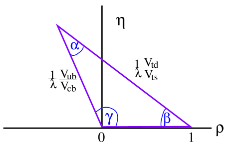
Figure 1: The unitarity triangle shown in the $\rho-\eta$ plane. The left side is determined by measurements of $b\to u/b\to c$ and the right side can be determined using mixing measurements in the $B_{s}$ and $B_{d}$ systems. The angles can be found by making measurements of CP violating asymmetries in hadronic $B$ decays.

We know the length of two sides already: the base is defined as unity and the left side is determined by the measurements of $|V_{ub}/V_{cb}|$, but the error is still quite substantial. The right side can be determined using mixing measurements in the neutral $B$ systems. Fig. 1 also shows the angles as $\alpha,~{}\beta$, and $\gamma$. These angles can be determined by measuring CP violation in the $B$ system.

Neutral $B$ mesons can transform to their anti-particles before they decay. The diagrams for $B_{d}$ mixing are shown in Fig. 2. (The diagrams for $B_{s}$ mixing are similar with $s$ quarks replacing $d$ quarks.) Although $u$, $c$ and $t$ quark exchanges are all shown, the $t$ quark plays a dominant role, mainly due to its mass, since the amplitude of this process is proportional to the mass of the exchanged fermion.

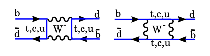
Figure 2: The two diagrams for $B_{d}$ mixing.

The probability of mixing is given by [10]

$$x\equiv\frac{\Delta m}{\Gamma}={G_{F}^{2}\over 6\pi^{2}}B_{B}f_{B}^{2}m_{B}\tau_{B}|V^{*}_{tb}V_{td}|^{2}m_{t}^{2}F{\left(m^{2}_{t}\over M^{2}_{W}\right)}\eta_{QCD},$$ (11)

where $B_{B}$ is a parameter related to the probability of the $d$ and $\bar{b}$ quarks forming a hadron and must be estimated theoretically; $F$ is a known function which increases approximately as $m^{2}_{t}$, and $\eta_{QCD}$ is a QCD correction, with value about 0.8. By far the largest uncertainty arises from the unknown decay constant, $f_{B}$. This number gives the coupling between the $B$ and the $W^{-}$. It could in principle be determined by finding the decay rate of $B^{+}\to\mu^{+}\nu$ or to $\tau^{+}\nu$, both of which are very difficult to measure.

$B_{d}$ mixing was first discovered by the ARGUS experiment [11]. (There was a previous measurement by UA1 indicating mixing for a mixture of $B_{d}^{o}$ and $B_{s}^{o}$ [12].) At the time it was quite a surprise, since $m_{t}$ was thought to be in the 30 GeV range. Since

$$|V^{*}_{tb}V_{td}|^{2}\propto|(1-\rho-i\eta)|^{2}=(\rho-1)^{2}+\eta^{2},$$ (12)

measuring mixing gives a circle centered at (1,0) in the $\rho-\eta$ plane.

The best recent mixing measurements have been done at LEP, where time-dependent oscillations have been measured. Averaging over all LEP experiments x=0.728$\pm$0.025 [13].

Another constraint on $\rho$ and $\eta$ is given by the $K_{L}^{o}$ CP violation measurement ($\epsilon$) [14]:

$$\eta\left[(1-\rho)A^{2}(1.4\pm 0.2)+0.35\right]A^{2}{B_{K}\over 0.75}=(0.30\pm 0.06),$$ (13)

where $B_{K}$ is parameter that cannot be measured and thus must be calculated. I use $0.9>B_{k}>0.6$ given by an assortment of theoretical calculations [14]; this number is one of the largest sources of uncertainty. Other constraints come from current measurements on $V_{ub}/V_{cb}$, and $B_{d}$ mixing [16]. The current status of constraints on $\rho$ and $\eta$ is shown in Fig. 3. The width of both of these bands are also dominated by theoretical errors. Note that the errors used are $\pm 1\sigma$. This shows that the data are consistent with the standard model but do not pin down $\rho$ and $\eta$.

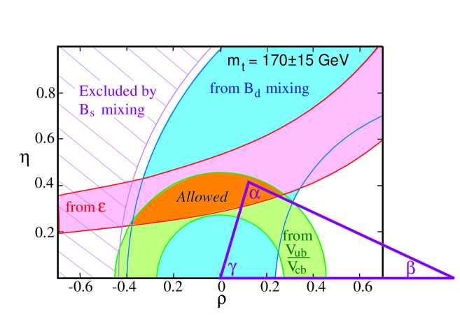
Figure 3: The regions in $\rho-\eta$ space (shaded) consistent with measurements of CP violation in $K_{L}^{o}$ decay ($\epsilon$), $V_{ub}/V_{cb}$ in semileptonic $B$ decay, $B_{d}^{o}$ mixing, and the excluded region from limits on $B_{s}^{o}$ mixing. The allowed region is defined by the overlap of the 3 permitted areas, and is where the apex of the CKM triangle sits. The bands represent $\pm 1\sigma$ errors. The large width of the $B_{d}$ mixing band is dominated by the uncertainty in the parameter $f_{B}$. Here the range is taken as $240>f_{B}>160$ MeV.

It is crucial to check if measurements of the sides and angles are consistent, i.e., whether or not they actually form a triangle. The standard model is incomplete. It has many parameters including the four CKM numbers, six quark masses, gauge boson masses and coupling constants. Perhaps measurements of the angles and sides of the unitarity triangle will bring us beyond the standard model and show us how these paramenters are related, or what is missing.

To get some idea of the size of the effects we need to deal with, I show in Fig. 4 the expectations for the three CP violating angles and $x_{s}$ plotted versus $\rho$. These plots merely reflect the “allowed” region shown in Fig. 3. It should be emphasized that this is not the result of a sophisticated analysis, which is difficult to do because of the non-Gaussian nature of the theoretical errors.

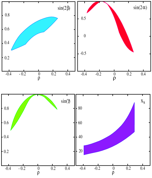
Figure 4: The allowed values of three CP violating angles and the $B_{s}$ mixing parameter $x_{s}$ as a function of $\rho$, taken from the allowed region in Fig. 3.

Furthermore, new physics can also be observed by measuring branching ratios which violate standard model predictions. Especially important are “rare decay,” processes such as $B\to K\mu^{+}\mu^{-}$ or $D\to\pi\mu^{+}\mu^{-}$. These processes occur only through “loops,” and are a class of what has become called “Penguin” decays.

2.2 Formalism of CP Violation in Neutral $B$ Decays

Consider the operations of Charge Conjugation, C, and Parity, P:

$$C|B(\overrightarrow{p})\big{>}=|\overline{B}(\overrightarrow{p})\big{>},~{}~{}~{}~{}~{}~{}~{}~{}~{} C|\overline{B}(\overrightarrow{p})\big{>}=|{B}(\overrightarrow{p})\big{>}$$ (14)

$$P|B(\overrightarrow{p})\big{>}=-|{B}(-\overrightarrow{p})\big{>},~{}~{}~{}~{}~{} P|\overline{B}(\overrightarrow{p})\big{>}=-|{B}(-\overrightarrow{p})\big{>}$$ (15)

$$CP|B(\overrightarrow{p})\big{>}=-|\overline{B}(-\overrightarrow{p})\big{>},~{}~{}~{} CP|\overline{B}(\overrightarrow{p})\big{>}=-|{B}(-\overrightarrow{p})\big{>}~{}~{}.$$ (16)

For neutral mesons we can construct the CP eigenstates

$$\big{|}B^{o}_{1}\big{>} = {1\over\sqrt{2}}\left(\big{|}B^{o}\big{>}-\big{|}\overline{B}^{o}\big{>}\right)~{}~{},$$ (17)

$$\big{|}B^{o}_{2}\big{>} = {1\over\sqrt{2}}\left(\big{|}B^{o}\big{>}+\big{|}\overline{B}^{o}\big{>}\right)~{}~{},$$ (18)

where

$$CP\big{|}B^{o}_{1}\big{>} = \big{|}B^{o}_{1}\big{>}~{}~{},$$ (19)

$$CP\big{|}B^{o}_{2}\big{>} = -\big{|}B^{o}_{2}\big{>}~{}~{}.$$ (20)

Since $B^{o}$ and $\overline{B}^{o}$ can mix, the mass eigenstates are a superposition of $a\big{|}B^{o}\big{>}+b\big{|}\overline{B}^{o}\big{>}$ which obey the Schrodinger equation

$$i{d\over dt}\left(\begin{array}[]{c}a\\ b\end{array}\right)=H\left(\begin{array}[]{c}a\\ b\end{array}\right)=\left(M-{i\over 2}\Gamma\right)\left(\begin{array}[]{c}a\\ b\end{array}\right).$$ (21)

If CP is not conserved then the eigenvectors, the mass eigenstates $\big{|}B_{L}\big{>}$ and $\big{|}B_{H}\big{>}$, are not the CP eigenstates but are

$$\big{|}B_{L}\big{>}=p\big{|}B^{o}\big{>}+q\big{|}\overline{B}^{o}\big{>},~{}~{}\big{|}B_{H}\big{>}=p\big{|}B^{o}\big{>}-q\big{|}\overline{B}^{o}\big{>},$$ (22)

where

$$p={1\over\sqrt{2}}{{1+\epsilon_{B}}\over{\sqrt{1+|\epsilon_{B}|^{2}}}},~{}~{}q={1\over\sqrt{2}}{{1-\epsilon_{B}}\over{\sqrt{1+|\epsilon_{B}|^{2}}}}.$$ (23)

CP is violated if $\epsilon_{B}\neq 0$, which occurs if $|q/p|\neq 1$.

The time dependence of the mass eigenstates is

$$\big{|}B_{L}(t)\big{>} = e^{-\Gamma_{L}t/2}e^{im_{L}t/2}\big{|}B_{L}(0)\big{>}$$ (24)

$$\big{|}B_{H}(t)\big{>} = e^{-\Gamma_{H}t/2}e^{im_{H}t/2}\big{|}B_{H}(0)\big{>},$$ (25)

leading to the time evolution of the flavor eigenstates as

$$\big{|}B^{o}(t)\big{>} = e^{-\left(im+{\Gamma\over 2}\right)t}\left(\cos{\Delta mt\over 2}\big{|}B^{o}(0)\big{>}+i{q\over p}\sin{\Delta mt\over 2}\big{|}\overline{B}^{o}(0)\big{>}\right)$$ (26)

$$\big{|}\overline{B}^{o}(t)\big{>} = e^{-\left(im+{\Gamma\over 2}\right)t}\left(i{p\over q}\sin{\Delta mt\over 2}\big{|}B^{o}(0)\big{>}+\cos{\Delta mt\over 2}\big{|}\overline{B}^{o}(0)\big{>}\right),$$ (27)

where $m=(m_{L}+m_{H})/2$, $\Delta m=m_{H}-m_{L}$ and $\Gamma=\Gamma_{L}\approx\Gamma_{H}$, and $t$ is the decay time in the $B^{o}$ rest frame, the so called proper time. Note that the probability of a $B^{o}$ decay as a function of $t$ is given by $\big{<}B^{o}(t)\big{|}B^{o}(t)\big{>}^{*}$, and is a pure exponential, $e^{-\Gamma t/2}$, in the absence of CP violation.

2.2.1 CP violation for $B$ via interference of mixing and decays

Here we choose a final state $f$ which is accessible to both $B^{o}$ and $\overline{B}^{o}$ decays [17]. The second amplitude necessary for interference is provided by mixing. Fig. 5 shows the decay into $f$ either directly or indirectly via mixing.

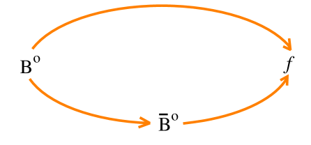
Figure 5: Two interfering ways for a $B^{o}$ to decay into a final state $f$.

It is necessary only that $f$ be accessible directly from either state; however if $f$ is a CP eigenstate the situation is far simpler. For CP eigenstates

$$CP\big{|}f_{CP}\big{>}=\pm\big{|}f_{CP}\big{>}.$$ (28)

It is useful to define the amplitudes

$$A=\big{<}f_{CP}\big{|}{\cal H}\big{|}B^{o}\big{>},~{}~{}\overline{A}=\big{<}f_{CP}\big{|}{\cal H}\big{|}\overline{B}^{o}\big{>}.$$ (29)

If $\left|{\overline{A}\over A}\right|\neq 1$, then we have “direct” CP violation in the decay amplitude, which we will discuss in detail later. Here CP can be violated by having

$$\lambda={q\over p}\cdot{\overline{A}\over A}\neq 1,$$ (30)

which requires only that $\lambda$ acquire a non-zero phase, i.e. $|\lambda|$ could be unity and CP violation can occur.

A comment on neutral $B$ production at $e^{+}e^{-}$ colliders is in order. At the $\Upsilon(4S)$ resonance there is coherent production of $B^{o}\bar{B}^{o}$ pairs. This puts the $B$’s in a $C=-1$ state. In hadron colliders, or at $e^{+}e^{-}$ machines operating at the $Z^{o}$, the $B$’s are produced incoherently [17]. For the rest of this article I will assume incoherent production except where explicitly noted.

The asymmetry, in this case, is defined as

$$a_{f_{CP}}={{\Gamma\left(B^{o}(t)\to f_{CP}\right)-\Gamma\left(\overline{B}^{o}(t)\to f_{CP}\right)}\over{\Gamma\left(B^{o}(t)\to f_{CP}\right)+\Gamma\left(\overline{B}^{o}(t)\to f_{CP}\right)}},$$ (31)

which for $|q/p|=1$ gives

$$a_{f_{CP}}={{\left(1-|\lambda|^{2}\right)\cos\left(\Delta mt\right)-2{\rm Im}\lambda\sin(\Delta mt)}\over{1+|\lambda|^{2}}}.$$ (32)

For the cases where there is only one decay amplitude $A$, $|\lambda|$ equals 1, and we have

$$a_{f_{CP}}=-{\rm Im}\lambda\sin(\Delta mt).$$ (33)

Only the amplitude, ${\rm-Im}\lambda$ contains information about the level of CP violation, the sine term is determined only by $B_{d}$ mixing. In fact, the time integrated asymmetry is given by

$$a_{f_{CP}}=-{x\over{1+x^{2}}}{\rm Im}\lambda=-0.48{\rm Im}\lambda~{}~{}.$$ (34)

This is quite lucky as the maximum size of the coefficient for any $x$ is $-0.5$.

Let us now find out how ${\rm Im}\lambda$ relates to the CKM parameters. Recall $\lambda={q\over p}\cdot{\overline{A}\over A}$. The first term is the part that comes from mixing:

$${q\over p}={{\left(V_{tb}^{*}V_{td}\right)^{2}}\over{\left|V_{tb}V_{td}\right|^{2}}}={{\left(1-\rho-i\eta\right)^{2}}\over{\left(1-\rho+i\eta\right)\left(1-\rho-i\eta\right)}}=e^{-2i\beta}{\rm~{}~{}and}$$ (35)

$${\rm Im}{q\over p}=-{{2(1-\rho)\eta}\over{\left(1-\rho\right)^{2}+\eta^{2}}}=\sin(2\beta).$$ (36)

To evaluate the decay part we need to consider specific final states. For example, consider $f\equiv\pi^{+}\pi^{-}$. The simple spectator decay diagram is shown in Fig. 6.

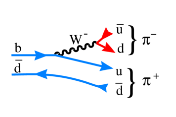
Figure 6: Decay diagram at the tree level for $B^{o}\to\pi^{+}\pi^{-}$.

For the moment we will assume that this is the only diagram which contributes. Later I will show why this is not true. For this $b\to u\bar{u}d$ process we have

$${\overline{A}\over A}={{\left(V_{ud}^{*}V_{ub}\right)^{2}}\over{\left|V_{ud}V_{ub}\right|^{2}}}={{(\rho-i\eta)^{2}}\over{(\rho-i\eta)(\rho+i\eta)}}=e^{-2i\gamma},$$ (37)

and

$${\rm Im}(\lambda)={\rm Im}(e^{-2i\beta}e^{-2i\gamma})={\rm Im}(e^{2i\alpha})=-\sin(2\alpha).$$ (38)

For our next example let’s consider the final state $\psi K_{S}$. The decay diagram is shown in Fig. 7. In this case we do not get a phase from the decay part because

$${\overline{A}\over A}={{\left(V_{cb}V_{cs}^{*}\right)^{2}}\over{\left|V_{cb}V_{cs}\right|^{2}}}$$ (39)

is real to order $1/\lambda^{4}$.

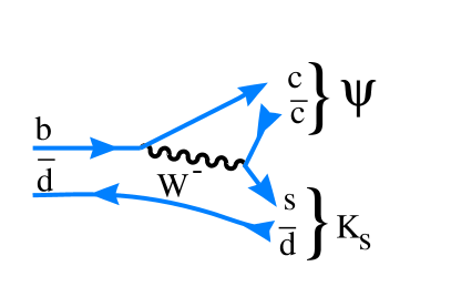
Figure 7: Decay diagram at the tree level for $B^{o}\to\psi K_{S}$.

In this case the final state is a state of negative $CP$, i.e. $CP\big{|}\psi K_{S}\big{>}=-\big{|}\psi K_{S}\big{>}$. This introduces an additional minus sign in the result for ${\rm Im}\lambda$. Before finishing discussion of this final state we need to consider in more detail the presence of the $K_{S}$ in the final state. Since neutral kaons can mix, we pick up another mixing phase (similar diagrams as for $B^{o}$, see Fig. 2). This term creates a phase given by

$$\left({q\over p}\right)_{K}={{\left(V_{cd}^{*}V_{cs}\right)^{2}}\over{\left|V_{cd}V_{cs}\right|^{2}}},$$ (40)

which is real to order $\lambda^{4}$. It necessary to include this term, however, since there are other formulations of the CKM matrix than Wolfenstein, which have the phase in a different location. It is important that the physics predictions not depend on the CKM convention.

In summary, for the case of $f=\psi K_{S}$, ${\rm Im}\lambda=-\sin(2\beta)$.

2.2.2 Comment on Penguin Amplitude

In principle all processes can have penguin components. One such diagram is shown in Fig. 8. The $\pi^{+}\pi^{-}$ final state is expected to have a rather large penguin amplitude $\sim$10% of the tree amplitude. Then $|\lambda|\neq 1$ and $a_{\pi\pi}(t)$ develops a $\cos(\Delta mt)$ term. It turns out that $\sin(2\alpha)$ can be extracted using isospin considerations and measurements of the branching ratios for $B^{+}\to\pi^{+}\pi^{o}$ and $B^{o}\to\pi^{o}\pi^{o}$, or other methods [23].

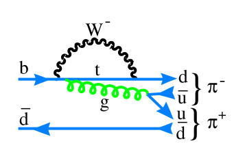
Figure 8: Penguin diagram for $B^{o}\to\pi^{+}\pi^{-}$.

In the $\psi K_{S}$ case, the penguin amplitude is expected to be small since a $c\bar{c}$ pair must be “popped” from the vacuum. Even if the penguin decay amplitude were of significant size, the decay phase is the same as the tree level process, namely zero.

2.3 Charm Physics Goals

According to the standard model, charm mixing and CP violating effects should be “small.” Thus charm provides an excellent place for non-standard model effects to a appear. Specific goals are listed below.

$\bullet$ Search for mixing in $D^{o}$ decay, by looking for both the rate of wrong sign decay, $r_{D}$ and the width difference between positive CP and negative CP eigenstate decays, $\Delta\Gamma$. The current upper limit on $r_{D}$ is $3.7\times 10^{-3}$, while the standard model expectation is $r_{D}<10^{-7}$ [20].

$\bullet$ Search for CP violation in $D^{o}$. Here we have the advantage over $b$ decays that there is a large $D^{*+}$ signal which tags the inital flavor of the $D^{o}$ through the decay $D^{*+}\to\pi^{+}D^{o}$. Similarly $D^{*-}$ decays tag the flavor of inital $\overline{D}^{o}.$ The current experimental upper limits on CP violating asymmetries are on the order of 10%, while the standard model prediction is about 0.1% [21].

$\bullet$ We also want to measure $\Delta\Gamma$, the lifetime difference between CP+ and CP- eigenstates. To do this we can measure the lifetime in the decay mode $D^{o}\to K^{+}K^{-}$, which is pure CP+ and compare it with the lifetime measured using $D^{o}\to K^{-}\pi^{+}$, which is an equal mixture of CP states.

$\bullet$ Search for rare decays of charm, which if found would signal new physics.

2.4 $b$ Physics Goals

We expect that the phase of $B_{d}$ mixing, called $\sin(2\beta)$, will have been measured prior to the advent of BTeV or LHC-B by at least one of the experiments: Babar, Belle, CDF or HERAB [22]. There is also a possibility of that a CP violating rate in flavor specific decays such as $B\to K^{-}\pi^{+}$ will have been seen. We do not however, expect that measurements will exist of our main physics goals, which are listed below:

$\bullet$ Measurement of the CP violating asymmetry in $B^{o}\to\pi^{+}\pi^{-}$. Penguin pollution may cause a problem for the extraction of the angle $\alpha$. There have been several theoretical suggestions of how to do this using additional branching ratios measurements [23].

$\bullet$ Measurment of mixing and CP violation in $B_{s}$ decays. The mass difference between “short” and “long” eigenstates can be determined measuring the flavor tagged time dependence of one or more of the final states $\psi K^{*o}$, $D_{s}^{+}\pi^{-}$ or $D_{s}^{+}\pi^{+}\pi^{-}\pi^{-}$. It is also possible that there is sizable $\Delta\Gamma$ in the $B_{s}$ system. Some estimates give $\Delta\Gamma\sim 0.1\times\Gamma$ [24]. This can be determined by measuring the lifetimes separately for CP+ and CP- eigenstates. For example, $D_{s}^{+}D_{s}^{-}$ is a CP+ eigenstate, while $\psi K_{s}$ is a CP- eigenstate. These final states are useful to look for a large non-standard model time dependent CP violating asymmetry, since in the standard model only small asymmetry is expected. Exquisit time resolution is required, since $B_{s}$ oscillation are expected to be quite rapid. Very importantly, time dependent measurements of the decays to the final states $D_{s}^{\pm}K^{\mp}$ can provide a direct measurement of the angle $\gamma$ [25]. Fig. 9 shows the two direct decay processes for $\overline{B}^{o}_{s}$. These interfere with the mixing induced processes.

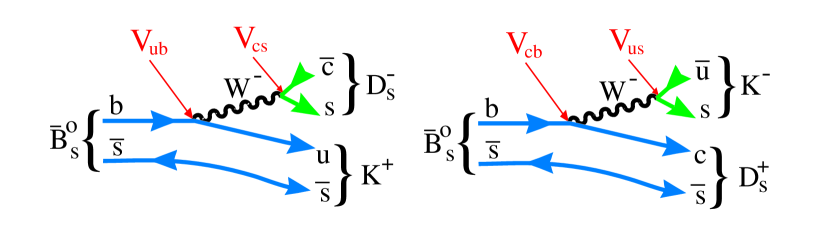
Figure 9: Two diagrams for $\overline{B}_{s}^{o}\to D_{s}^{\pm}K^{\mp}$.

$\bullet$ Measurement of rare decay processes such as $B^{o}\to K^{+}\pi^{-}$, $B\to K\ell^{+}\ell^{-}$, etc…

$\bullet$ Precision measurement of $\sin(2\beta)$ using $\psi K_{s}$.

$\bullet$ Precision measurements of $V_{ub}/V_{cb}$ and $V_{cb}$ using both meson and baryon decays such as $\Lambda_{b}\to p\ell\nu.$

3 Characteristics of Hadronic $b$ Production

It is often customary to characterize heavy quark production in hadron collisions with the two variables $p_{t}$ and $\eta$. The later variable was first invented by those who studied high energy cosmic rays and is assigned the value

$$\eta=-ln\left(\tan\left({\theta/2}\right)\right),$$ (41)

where $\theta$ is the angle of the particle with respect to the beam direction.

According to QCD based calculations of $b$ quark production, the $b$’s are produced “uniformly” in $\eta$ and have a truncated transverse momentum, $p_{t}$, spectrum, characterized by a mean value approximately equal to the $B$ mass [26]. The distribution in $\eta$ is shown in Fig. 10.

Figure 10: The $B$ yield versus $\eta$ (left). $\beta\gamma$ of the $B$ versus $\eta$ (right). Both plots are for the Tevatron.

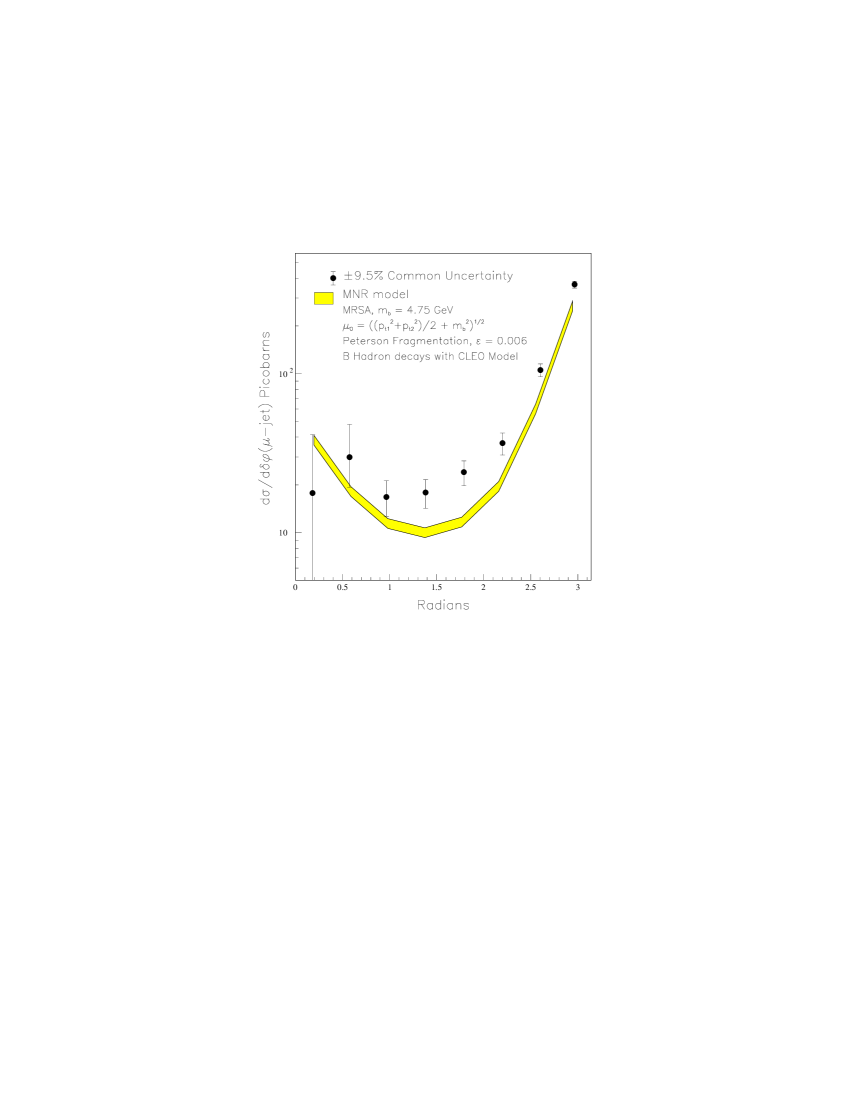
Figure 11: The differential $\delta\phi$ cross-sections for $p^{\mu}_{T}>9$ GeV/c, $\left|\eta^{\mu}\right|<$0.6, E${}^{\bar{b}}_{T}>$10 GeV, $\left|\eta^{\bar{b}}\right|<1.5$ compared with theoretical predictions. The data points have a common systematic uncertainty of $\pm$9.5%. The uncertainty in the theory curve arises from the error on the muonic branching ratio and the uncertainty in the fragmentation model.

There is a strong correlation between the $B$ momentum and $\eta$. Shown also in Fig. 10 is the $\beta\gamma$ of the $B$ hadron versus $\eta$. It can clearly be seen that near $\eta$ of zero, $\beta\gamma\approx 1$, while at larger values of $|\eta|$, $\beta\gamma$ can easily reach values of  6. This is important because the observed decay length varies with $\beta\gamma$ and furthermore the absolute momenta of the decay products are larger allowing for a supression of the multiple scattering error.

Since the detector design is somewhat dependent on the Monte Carlo generated $b$ production distributions, it is important to check that the correlations between the $b$ and the $\overline{b}$ are adequately reproduced. In Fig. 11 I show the azimuthal opening angle distribution between a muon from a $b$ quark decay and the $\bar{b}$ jet as measured by CDF [27] and compare with the MNR predictions [28].

The model does a good job in representing the shape which shows a strong back-to-back correlation. The normalization is about a factor of two higher in the data than the theory, which is generally true of CDF $b$ cross-section measurements [29]. In hadron colliders all $B$ species are produced at the same time.

The “flat” $\eta$ distribution hides an important correlation of $b\bar{b}$ production at hadronic colliders. In Fig. 12 the production angles of the hadron containing the $b$ quark is plotted versus the production angle of the hadron containing the $\bar{b}$ quark according to the Pythia generator (for the Tevatron). There is a very strong correlation in the forward (and backward) direction: when the $B$ is forward the $\overline{B}$ is also forward. This correlation is not present in the central region (near zero degrees). By instrumenting a relative small region of angular phase space, a large number of $b\bar{b}$ pairs can be detected. Furthermore the $B$’s populating the forward and backward regions have large values of $\beta\gamma$.

Figure 12: The production angle (in degrees) for the hadron containing a $b$ quark plotted versus the production angle for a hadron containing $\bar{b}$ quark. (For the Tevatron.)

Charm production is similar to $b$ production but much larger. Current theoretical esitmates are that charm is 1-2% of the total $p\bar{p}$ cross-section. Table  3 gives the relevant parameters for the Tevatron and LHC. BTeV expecst to start serious data taking in Fermilab Run II with a luminosity of about $5\times 10^{31}$cm^-2s^-1; the ultimate luminosity goal, to be obtained in Run III is $2\times 10^{32}$cm^-2s^-1.

Table 1: Properties of the Tevatron and LHC as a $b$ and $c$ sources.

1.5cmlcc Property Fermilab (Run II) LHC-B

Luminosity $0.5\times 10^{32}$cm^-2s^-1 $[\dagger]$ $1.5\times 10^{32}$cm^-2s^-1

$b$ cross-section 100 $\mu$b 500 $\mu$b

# of $b$’s per 10⁷ sec $10^{11}$ $5\times 10^{11}$

$b$ fraction 0.2% 0.5%

$c$ cross-section $>500~{}\mu$b $>4000~{}\mu$b

Bunch spacing 132 ns 25 ns

Luminous region length $\sigma_{z}$ = 30 cm 5.3 cm

Luminous region width $\sigma_{x}$=$\sigma_{y}$ $\approx$ 50 $\mu$m $\sigma_{x}$=$\sigma_{y}$ = 70 $\mu$m

Interactions/crossing $<0.5>$ $<0.4>$

$\dagger$ The ultimate luminosity for BTeV is projected to be $2\times 10^{32}$cm^-2s^-1.

4 Designs of LHC-B and BTeV

4.1 Introduction

Both dedicated $B$ detectors have decided to use the “forward” direction. There are several reasons for this. First of all, it is possible to get a signficant fraction of events with both the $b$ and $\overline{b}$ in the detector. Secondly, the geometry allows space for charged particle identification. Thirdly, it is possible to place a microvertex detector inside the main beam pipe and retract it during machine fills, necessary to minimize radiation damage. A test of this concept was done at CERN by experiment P238 [30]. A sketch of their silicon detector arrangement is shown in Fig. 13.

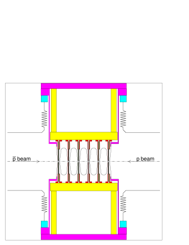
Figure 13: Side view of the P238 silicon detector assembly and Roman pots. The 6 silicon planes are the vertical lines just above and below the beam line. The bellows (zig-zag lines) allow movements in the vertical direction of the pots, which are the thin vertical lines close to the bellows (they have 2 mm wall thickness). The edges of the 200 $\mu$m-thick aluminum RF shields closest to the beam (shown as the thin curved lines near the silicon detectors) normally ran at a distance of 1.5 mm from the circulating beams. The black horizontal pieces at top and bottom are the vacuum bulkheads bolted to the Roman pots.

Since in hadron-hadron interactions there are many more hadronic interactions than interesting events, it is necessary to select which events to keep for further processing. In normal parlance this is called “triggering the experiment.” The implementation of the trigger is crucial to the success of any hadronic $b$ experiment. BTeV is designed around the ability to trigger on the detached vertex created by the decay of hadron containing a $b$ or $c$ quark. BTeV and LHC-B also have the ability to trigger on events with opposite sign $e^{+}e^{-}$ or $\mu^{+}\mu^{-}$ pairs. Because of the specific design of its microvertex detector, LHC-B cannot do a detached vertex trigger in the first level lest they be swamped with too high a trigger rate [31]. They require that they have either electrons, muons or hadrons at moderate $p_{t}$ before they look for the consequences of a detached vertex. These requirement causes a loss of efficiency which depends on the charged multiplicity of the final state.

Both experiments have excellent charged hadron identification, and lepton identification as well as excellent momentum resolution. Neither experiment has investigated in detail the efficacy of using photons or neutral pions. I will assume, conservatively, in this paper that they cannot be used.

4.2 The BTeV Design

A sketch of the BTeV apparatus is shown in Fig. 14. The plan view shows the two-arm spectrometer fitting in the expanded C0 interaction region at Fermilab. The magnet, called SM3, exists at Fermilab. The other important parts of the experiment include the vertex detector, the RICH detectors, the EM calorimeters and the muon system. The solid angle subtended is approximately $\pm$300 mr in both plan and elevation views.

Figure 14: Sketch of the BTeV spectrometer.

The C0 interaction region at Fermilab will be enlarged and a counting room constructed starting around Nov. 15, 1997. It will be completed before the main injector turns on.

4.2.1 The BTeV pixel vertex detector

The vertex detector is a multiplane pixel device which sits inside the beam pipe. A sketch is shown in Fig. 15. This detector is the most versatile part of the experiment. It is used for precise measurement of the vertex position of the primary $p\overline{p}$ interaction and heavy quark decay vertices. It is the key element of the detached vertex trigger and it is an integral part of the charged particle momentum measuring system.

Data is “pipelined” out of the detector and kept in temporary storage until a decision can be made on wether or not there is a detached $b$ or $c$ vertex. The vertex detector is put in the magnetic field in order to insure that the tracks considered for vertex based triggers do not have large mulitple scattering because they are low momentum.

Figure 15: Sketch of the pixel vertex detector for BTeV.

Simulations have been carried out taking as a baseline detector triplets of pixels with dimension 30 $\mu$m x 300 $\mu$m. The function of the triplet is to provide a track vector in the bend plane, along with a three dimensional spacial coordinate. This useful in making the trigger algorithm fast. These pixel dimensions are the minimum BTeV is considering using. Studies are underway to see how much bigger the pixels can be without degrading the performance. Also, the minimum distance of the detector to the beam line is set at 6 mm, though the beam size is small enough that a smaller distance could be considered.

In addition to the pixel detector, the charged particle tracking system contains several planes of wire or straw chambers. These are particularly necessary to provide excellent momentum resolution and to reconstruct $K_{s}^{o}$ decays into $\pi^{+}\pi^{-}$

4.2.2 Particle Identification

Excellent charged hadron identification is a critical component of a heavy quark experiment. Even for a spectrometer with the excellent mass resolution of BTeV, there are kinematic regions where signals from one final state will overlap those of another final state. For example, $B_{d}^{o}\rightarrow\pi^{+}\pi^{-}$, $B_{d}^{o}\rightarrow K^{+}\pi^{-}$, and $B_{s}^{o}\rightarrow K^{+}K^{-}$ all overlap to some degree. These ambiguities can be eliminated almost entirely by an effective particle identifier. In addition, many physics investigations involving neutral $B$-mesons require ‘tagging’ of the flavor of the signal particle by examining the properties of the ‘away-side’ particle. Kaon tagging is a very effective means of doing this.

In the design of any particle identification system, the dominant consideration is the momentum range over which efficient separation of the charged hadron species $\pi$, $K$, and $p$ must be provided. The upper end of the momentum requirement is given by two-body decays such as $B\rightarrow\pi^{+}\pi^{-}$ which produce the highest momentum particles in $b$ decays. Fig. 16 shows the momentum distribution of pions from the decay $B_{d}^{o}\rightarrow\pi^{+}\pi^{-}$ for the case where the two particles are within the spectrometer’s acceptance.

The low momentum requirement is defined by having high efficiency for ‘tagging’ kaons from generic B decays. Since these kaons come mainly from daughter $D$ mesons in multibody final state $B$ decays, they typically have much lower momentum than the particles in two-body decays. Fig. 17 shows the momentum distribution of ‘tagging’ kaons for the case where the signal particles are within the geometric acceptance of the spectrometer. About 1/5 of the tagging kaons never exit the end of the spectrometer dipole. Almost all of them are below 3 GeV, and most kaons exiting the dipole have momenta above 3 GeV. Based on these considerations, the momentum range requirement for the particle identification system is defined as separating kaons from pions between 3 and 70 GeV/c.

Kaons and pions from directly produced charm decays have momenta which are not very different from the kaons from $B$-decays. Fig. 18 shows the momentum spectra of kaons from accepted $D^{o}\rightarrow K^{-}\pi^{+}$, $D^{o}\rightarrow K^{-}\pi^{+}\pi^{-}\pi^{+}$, and $D_{s}^{+}\rightarrow K^{+}K^{-}\pi^{+}$ in both collider and fixed target mode. The range set by the $B$-physics requirements is a reasonable choice for charm physics.

Figure 16: The momentum distribution of pions in $B_{d}\to\pi^{+}\pi^{-}$ decays. The left plot shows distributions for the lower (dashed line) and higher (solid line) momentum pion in this decay. The right plot presents the later distribution in integral form, which gives loss of efficiency as a function of the high momentum cut-off of the particle ID device.

Figure 17: The momentum distribution of ‘tagging’ kaons for the case where the signal particles ($\psi K^{0}_{S}$) are within the geometric acceptance of the spectrometer. The left plot shows distributions for kaons absorbed in (dashed line) and exiting from (solid line) the magnet. The right plot presents the later distribution in integral form, which gives loss of efficiency as a function of the low momentum cut-off of the particle ID device.

Figure 18: The momentum spectra of kaons from accepted $D^{o}\rightarrow K^{-}\pi^{+}$, $D^{o}\rightarrow K^{-}\pi^{+}\pi^{-}\pi^{+}$, and $D_{s}^{+}\rightarrow K^{+}K^{-}\pi^{+}$ in both collider and fixed target modes.

Because of the large momentum range and limited longitudinal space available for a particle identification system in the C0 enclosure, the only sensible of detector technology is a gaseous ring-imaging Cherenkov counter. Fortunately, there are atmospheric pressure gas radiators which provide signal separation between pions and kaons in this momentum region. Table 4.2.2 gives some parameters for two candidate radiator gases: $C_{4}F_{10}$ and $C_{5}F_{12}$. Note that below 9 GeV, these gases do not provide $K/p$ separation since kaons are below threshold. $C_{5}F_{12}$ is used in the barrel part of the DELPHI RICH and in SLD (mixed with 15% N₂). It needs to be operated at $40^{o}$C because of its high condensation point. The $C_{4}F_{10}$ gas can be used at room temperature. It is used in the DELPHI endcap RICH and was adopted for the HERA-B and LHC-B RICH detectors.

1.5cmccc Parameter $C_{4}F_{10}$ $C_{5}F_{12}$

(n-1) x $10^{6}$ 1510 1750

gamma-threshold 18.2 16.9

$\Theta_{c}$($\beta$=1) 54.9 mr 59.1 mr

$\pi$ threshold 2.5 GeV/c 2.4 GeV/c

$K$ threshold 9.0 GeV/c 8.4 GeV/c

$p$ threshold 17.1 GeV/c 15.9 GeV/c

Table 2: Parameters of the two candidate Cherenkov gas radiators.

The visible light photons can be detected either with a new device called Hybrid Photo-diodes, HPD, or multi-anode PMTs such as the 16 channel tubes from Hamamatsu used in the HERA-B detector [32].

In order to increase positive identification of low momentum particles, one interesting possibility is to insert a thin ($\sim 5$ cm) piece of aerogel at the entrance to the gas RICH as proposed by LHC-B [33]. For example, aerogel with refractive index of $n=1.03$ would lower the $\pi$, $K$, $p$ momentum thresholds to $0.6$, $2.0$, $3.8$ GeV/c respectively. Shorter wavelength Cherenkov photons undergo Raleigh scattering inside the aerogel itself. They are absorbed in the radiator or exit at random angles. A thin mylar or glass window between the aerogel and the gas radiator would pass photons only in the visible range, eliminating the scattered component. The same photodetection system could then detect Cherenkov rings produced in both the gaseous and the aerogel radiators. The radius of rings produced in the aerogel would be about 4.5 times larger than those produced in $C_{4}F_{10}$. The aerogel radiator would provide positive $\pi/K$ separation up to 10-20 GeV/c. It would also close the lower momentum gap in $K/p$ separation. Since the low momentum coverage would be provided by aerogel, one could think about boosting the high momentum reach of the gas radiator by switching to a lighter gas such as $C_{2}F_{6}$ ($n=1.0008$) or $C\,F_{4}$ ($n=1.0005$). This would also loosen the requirements for Cherenkov angle resolution needed to reach a good $K/\pi$ separation at a momentum of 70 GeV/c. Detailed simulations are needed to evaluate trade-offs due to more complicated pattern recognition.

The alternative options to be considered for improving particle identification at lower momenta include a time-of-flight system or a DIRC.

4.2.3 Electron, photon and muon detection

BTeV is considering the use of a cryrogenic liquid based EM calorimeter. One solution uses a detector filled with liquid Krypton, similar to the one being used in NA48 [36]. This would provide the best possible position and energy resolution. It would in all probability only be used if there were processes where photons or $\pi^{o}$’s could be usefully reconstructed. A cheaper alternative, which is probably adequate for electron identification is a lead-liquid Argon detector. The liquid based detectors are naturally radiation hard.

4.2.4 The detached vertex trigger

BTeV places the vertex detector in the magnetic field to allow the elimination of low momentum tracks in the trigger. These tracks have large multiple scattering and can appear to come from detached verticies, thus fooling the trigger.

The goal of the trigger algorithm is to reconstruct tracks and find vertices in every interaction up to an interaction rate of order 10 MHz (luminosity of $10^{32}$ cm^-2 s^-1 at $\sqrt{s}=2$ TeV). This entails an enormous data rate coming from the detector ($\sim 100\,$GB/s), thus a careful organization of the data-flow is crucial. This trigger must be capable of reducing the event rate by a factor between a hundred and a thousand in the first level.

The key ingredients for such a trigger are a vertex detector with excellent spatial resolution, fast readout, and low occupancy; a heavily pipelined and parallel processing architecture well suited to tracking and vertex finding; inexpensive processing nodes, optimized for specific tasks within the overall architecture; sufficient memory to buffer the event data while the calculations are carried out; and a switching and control network to orchestrate the data movement through the system.

The detailed reference trigger scheme proposed for BTeV was developed by the Univ. of Pennsylvania Group [37]. While it may undergo some revisions, it has been an excellent starting point for studying this kind of trigger and the initial results for this particular algorithm are very encouraging.

The proposed algorithm has four steps (see Fig. 19):

In the first step, hits from each pixel plane are assigned to detector subunits. It is desirable to subdivide the area of the detectors in a way which minimizes the number of tracks crossing from one subunit into the next and assures uniform and low occupancy ($<1$ hit/event) in all subunits. Therefore each plane is divided into 32 azimuthal sectors (“$\phi$-slices”). Simulation shows that at 2 TeV, on average each $\phi$-slice contains 0.2 hits per inelastic interaction, approximately independent of the plane’s $z$ coordinate.

In the second step, “station hits” are formed in each triplet of closely-spaced planes using hits from each $\phi$-slice. Since the pixels under consideration have a rectangular shape (e.g. 30 $\mu$m by 300 $\mu$m), the two outer planes in each station are oriented for best resolution in the bend view, and the inner plane for the non-bend view. There is a “hit processor” for each $\phi$-slice of each station. The hit processor finds triplets of overlapping pixels, and sends to the next stage a single “minivector” consisting of $x$, $y$, $\frac{dx}{dz}$ and $\frac{dy}{dz}$. Given the good position resolution of each measurement, a detector station determines a space point accurate to $5-9\,\mu$m in $x$ and $y$, and $y$ and $x$ slopes to $\frac{dy}{dz}\approx 1\,$mr (bend-view) and $\frac{dx}{dz}\approx 10\,$mr (non-bend). The use of these minivectors in the track-finding stage substantially reduces combinatorics.

In the third step, minivectors in each $\phi$-slice from the full set of stations are passed via a sorting switch to a farm of “track processors.” The sign of the bend-view slope is used to distinguish forward-going and backward-going minivectors and send them to separate farms. To handle the few percent of tracks crossing segment boundaries, hits near a boundary between two $\phi$-slices can be sent to the processors for both slices. Each track processor links minivectors into tracks, proceeding along $z$ from station to station. For each pair of minivectors in adjacent stations, the processor averages the $y$-slopes in the two stations and uses this average slope (which represents the slope of the chord of the magnetically deflected trajectory) to project from the first station into the second. It then checks whether the $y$-value of the minivector in the downstream station agrees with the projection within an acceptance window. If three or more hits satisfy this requirement, a fast fitting algorithm finds the momentum of the track candidate.

In the fourth step, the tracks are passed to a farm of “vertex processors” and used to form vertices. The vertex with $\sum{p_{z}}$ closest to zero is designated as the primary vertex. Tracks which have a large impact parameter with respect to this vertex are taken as evidence for heavy quark production in an event. To reduce the effect of multiple scattering on vertex resolution, tracks below an adjustable bend-view transverse-momentum ($p_{y}$) threshold are excluded from the vertex finding.

Figure 19: Schematic of Proposed Level I vertex trigger

4.2.5 Beyond the Level I Trigger

Modern experiments in High Energy physics implement hierarchical trigger systems and BTeV is no exception. Many details of the full data acquisition system have to be worked out as the design of the detector components and trigger algorithms become more mature. At the design luminosity of $\rm 5\times 10^{31}cm^{-2}s^{-1}$ and with a total inelastic cross section of $\sigma_{inel}\approx 60$ mb the interaction rate at BTeV will be around 3 MHz. Fig. 20 gives the outline of the expected data flow at the nominal design luminosity.

Figure 20: The BTeV data flow diagram. The numbers are for the nominal luminosity of $\rm 5\times 10^{31}cm^{-2}s^{-1}$.

The Level I trigger must be capable of reducing the trigger rate by a factor between a hundred and a thousand. This seems to be achievable even if the only test made is for a detached vertex in vacuum. The event rate is then reduced to $\approx$100 kHz in the worst case during the highest luminosity running. It is still possible to move all this data, amounting to a maximum rate of 10 GB/s, to the Level II trigger.

Events that pass the first trigger level are forwarded to compute nodes to be further analyzed. First, detector component information is used to partially reconstruct the event, e.g. finding tracks in the vertex detector. Algorithms with refined secondary vertex requirements or invariant mass cuts will be implemented at this level. Events remaining after this step are then fully assembled in a switch-based eventbuilder and passed to a processor farm. Alternatively, an algorithm such as associating a mass with each detached vertex can be computed at Level I which would eliminate the need for an intermediate trigger step before the eventbuilder. Since most of the detached-vertex events will be $K_{s}$, a requirement that the mass at the vertex be above some threshold (say 1 GeV/c²) could reduce the rate to less than 10 kHz with almost no bias against charm and beauty events of interest. Even so, it will probably be impractical to write several kHz of events to archival storage.

The final trigger level will combine information from different sub-detectors to further suppress background events. Particle identification will be available at this stage and could be used to obtain a very clean direct charm signal for specific final states.

Because the event rate surviving this last level may still be close to a kHz, the software will probably have to reduce the amount of data per event to archival storage by writing out an event summary which eliminates much of the raw data. The event summary would be around 20 KB so that the output rate could still be as high as 20 MB/s. This results in a dataset size of 200 TB/yr, comparable to what is expected from CDF or D0 in Run II. However, initial phases of the experiment will run at much lower rates and will be comparable in dataset size to a current fixed target experiment.

4.2.6 Trigger simulations

Track hits are generated with multiple scattering and energy loss properly taken into account. The beam width is taken as $50~{}\mu m$ r.m.s., in both coordinates travsverse to the beam and the interaction region length is taken as 30 cm r.m.s. The reconstruction program does the full pattern recognition starting with hits on the pixel planes. Hits are formed into tracks, using the $\phi$ slices as discussed above, and the track momenta are calculated. The algorithm allows rejection of all tracks whose momentum in the bend plane, $p_{y}$, is less than a fixed cut. All the results shown here are for $p_{y}>0.5$ GeV/c, though this cut has not been optimized.

This algorithm is preliminary and can be imporved. The current simulation does not take into account Molière multiple-scattering tails, the effect of pair-conversions or hadronic interactions in the silicon, detector inefficiencies, or noise in the detector. The trigger performance has only been studied when there is one interaction per crossing. There are several ideas on how to handle the situation with more than one interaction.

The trigger algorithm first finds a primary interaction vertex. The distance a track misses the primary is then determined in units of $n\sigma$, where $\sigma$ refers to the r.m.s. error for a particular track distance to the primary. Then the number of tracks which miss the primary by $n\sigma$ is determined. Fig 21 shows the efficiency for triggering light quark ($uds$) background events as a function of both the number of tracks required and the specfic $n\sigma$ cut. The efficiency to trigger on a $B^{o}\to\pi^{+}\pi^{-}$ is also shown for events with both tracks in the detector.

Figure 21: Trigger efficiency of light quark background (left) and for $B^{o}\to\pi^{+}\pi^{-}$ events (right), both shown on the ordinate. The efficiency for the $\pi^{+}\pi^{-}$ plot is for events with tracks both required to be in the solid angle of the detector. The abscissa gives the value of the impact parameter in terms of number of standard deviations ($\sigma$) of the track from the primary vertex. The curves show the effect of requiring different numbers of tracks. All tracks are required to have at least 0.5 GeV/c momentum in the bend plane.

When the experiment runs one value of $n\sigma$ and one value of the number of tracks needs to be chosen. Values of 3$\sigma$ and 2 tracks provides an efficiency, in the spectrometer, of 43% for this process with a rejection of 125:1 against light quark background. The final cut values must be chosen with reference to many processes, however.

The trigger efficiency on states of interest is correlated with the analysis criteria used to reject background. These criteria generally are focussed upon insuring that that the $B$ decay track candidates come from a detached vertex, that the momentum vector from the $B$ would point back to the primary interaction vertex, and that there aren’t any other tracks which are consistent with $B$ vertex. When these criteria are applied first and the trigger efficiency estimated after, the trigger efficiency appears to be larger. In Fig. 22 I show the efficiency to trigger on $B_{s}\to\psi K^{*o}$, $\psi\to\mu^{+}\mu^{-}$, $K^{*o}\to K^{-}\pi^{+}$ using the tracking trigger only for events with the four tracks in the geometric acceptance, and the efficiency evaluated after all the analysis cuts have been applied. Here the trigger efficiencies for $3\sigma$ and 2 tracks are 67% for events with all 4 tracks in the geometrical acceptance and 84% on events after all the analysis cuts have been applied.

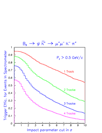
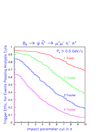
Figure 22: Trigger efficiency of $B_{s}\to\psi K^{*o}$, $\psi\to\mu^{+}\mu^{-}$, $K^{*o}\to K^{-}\pi^{+}$ for tracks in the geometric acceptance(left) and after all analysis cuts (right). The abscissa gives the value of the impact parameter in terms of number of standard deviations ($\sigma$) of the track from the primary vertex. The curves show the effect of requiring different numbers of tracks. All tracks are required to have at least 0.5 GeV/c momentum in the bend plane.

4.3 The LHC-B design

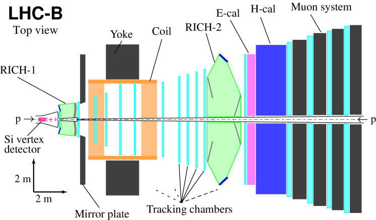
Figure 23: Overview of the LHC-B detector.

I will not give as an extensive discussion of the LHC-B design as I have done for BTeV, as the fundamental design concepts are quite similar. The LHC-B detector schematic is shown in Fig. 23.

There are several significant differences between LHC-B and BTeV. LHC-B is a single arm device. It also includes a hadron calorimeter, which BTeV lacks. The hadron calorimeter is used in the trigger for rejecting events with multiple primary interactions. The interaction region length is much smaller at LHC than at the Tevatron, so the vertex detector can be smaller. However, the LHC-B vertex detector is outside the magnetic field. Furthermore, since there is a RICH detector between the vertex detector and the magnetic, most of the momentum information comes from the tracking chambers alone. The vertex detector current is designed as silcon strips. There is a second RICH detector to indentify the higher momentum tracks.

4.3.1 The vertex detector

The LHC-B vertex detector contains 18 superlayers containing one $r$ strip detector and one $\phi$ strip detector. The arangement of superlayers is shown in Fig. 24. The strip arrangements on the individual detectors is shown in Fig. 25. The segmentation is increased closer to the beam line because the occupancies are higher there.

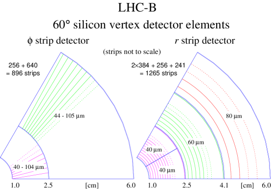
Figure 24: Overview of the LHC-B vertex detector.

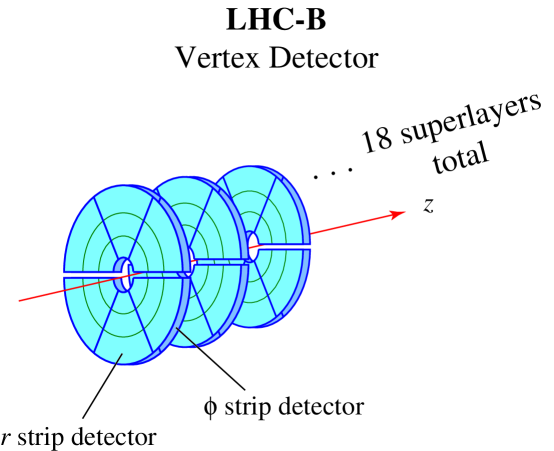
Figure 25: Details of the LHC-B silicon strip vertex detector.

4.3.2 The RICH detectors

LHC-B has two RICH detectors to cover the large momentum range. They are shown in Fig. 26. The both use HPD’s as photon detectors. The first one, located before the magnet and after the silicon detector has large acceptance for charged hadrons. It uses a C₄F₁₀ gas radiator and possibly an aerogel radiator. The light is mirrored to photon detectors out of the acceptance. The second RICH uses a lower index gas, CF₄ to identify higher momentum hadrons, more concentrated at smaller angles with respect to the beam. There is a double mirror system to keep the photon detectors out of the overall acceptance.

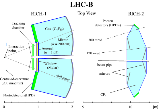
Figure 26: Schematic of the LHC-B RICH detectors. The scale on the bottom gives the location with respect to the center of the interaction region.

4.3.3 Calorimeters and Muon detector

The electromagnetic calorimeter has not been completely specified. One possibility is to have an inner part made of radiation hard PbWO₄ crystals, with the outer part be a a lead-scintillator “Shaslik” system. A “preshower” detector is also envisaged whos function is to reject photons in the electron trigger.

The hadron calorimeter also could have an inner and outer dicotomy. The inner part which needs high radiation resistance may possibly be constructed with tungsten plates and quartz as the active material generating Cherenkov light. The outer part could be alternating plates of steel and plastic scintillator.

The Muon detector consists of three 70 cm thick iron slabs with tracking chambers placed downstream of the hadron calorimeter.

5 Simulations

5.1 Introduction

I will give the results of several simulations done for BTeV. There are LHC-B simulations which can be found in their Letter of Intent [34].

BTeV has developed several fast simulation packages to verify the basic concepts and aid in the final design. Collisions are generated using either Pythia 5.7 or Jetset 7.4. Beauty and Charm decays are modeled using the CLEO decay generator QQ. Charged tracks are generated and traced through different material volumes including detector resolution, multiple scattering and efficiency. This allows measurement of acceptances and resolutions in a fast reliable manner. Pattern recognition has not been implemented. The key program is called MCFast [35].

5.2 Flavor tagging

5.2.1 Introduction

In order to measure CP violation or mixing in a neutral $B$ decay, it is essential that it be know if the intial particle was a $B$ or $\overline{B}$. Since hadrons containing $b$ quarks are produced in pairs in $e^{+}e^{-}$ and $p\overline{p}$ collisions, and thought to be in $pp$ interactions, one way to accomplish this “tagging” is to measure the $b$ content (flavor) of the other produced $B$. It is easiest to view the problem in the $p\overline{p}$ situation. Here if a $\overline{B}^{o}$ is produced the acompanying particle is either a $B^{+}$, $\Lambda_{b}$ or other baryonic state, $B^{o}$, or $B_{s}$. Since the $B^{+}$ doesn’t mix, its flavor at production is same as when it decays. The neutrals $B$’s, however, do mix and this dilutes the purity of the information. In fact, about 20% of the $B^{o}$’s turn up as $\overline{B}^{o}$ and 50% of the $B_{s}$’s turn up as $\overline{B}_{s}$. In $e^{+}e^{-}$ annihilations at the $\Upsilon$(4S), only $B^{o}$ is produced in conjunction with $\overline{B}^{o}$, and there are quantum correlation effects which need to be taken into consideration to understand the dilution due to mixing [17].

Another method of tagging is to use information from the fragmentation of the jet which produced the $B^{o}$. The clearest example of this occurs in charm. A $D^{*+}$ is produced which decays into $\pi^{+}D^{o}$. The $\pi^{+}$ tags the flavor of the $D^{o}$. A $\overline{D}^{o}$ would be tagged by a $\pi^{-}$. Unfortunately in the $B$ case, the $B^{*}$ is not massive enough to decay into a charged pion and decays only via a photon. There is however a $B^{**}$ state which can decay into a charged pion and a $B^{o}$. It is also possible to try and find the charge of pion closest in phase space to the $B^{o}$. These techniques are called “same side tagging.”

Beside mixing effects, dilution will occur because of incorrect tagging proceedures. The following definitions will be useful:

• $N\equiv$ number of reconstructed signal events we wish to tag.

• $N_{R}\equiv$ number of right sign flavor tags.

• $N_{W}\equiv$ number of wrong sign flavor tags.

• $\epsilon=\left(N_{R}+N_{W}\right)/N$, this is the efficiency.

• $D=(N_{R}-N_{W})/(N_{R}+N_{W}),$ this is the dilution.

The quantity that enters directly in calculating the error on any particular asymmetry measurement is $\epsilon D^{2}$.

5.2.2 Kaon tags

The decay chain $\overline{B}\to D\to K^{-}$ can be used to tag flavor. BTeV has investigated the feasiblity of tagging kaons using a gas Ring Imaging Cherenkov Counter (RICH) in a forward geometry and compared it with what is possible in a central geometry using Time-of-Flight counters with good, 100 ps, resolution. For the forward detector the momentum coverage required is between 3 and 70 GeV/c. The momentum range is much lower in the central detector but does have a long tail out to about 5 GeV/c. Fig. 27 shows the number of identified kaons plotted versus their impact parameter divided by the error in the impact parameter for both right sign and wrong sign kaons. A right sign kaon is a kaon which properly tags the flavor of the other $B$ at production. We expect some wrong sign kaons from mixing and charm decays. Many others just come from the primary. A cut on the impact parameter standard deviation plot at $3.5\sigma$ gives an overall $\epsilon D^{2}$ of 6%. This may be an over-estimate because proton fakes can be in the sample. Putting these in lowers $\epsilon D^{2}$ to 5.1%. These numbers are for a perfect RICH system. Putting in a fake rate of several percent, however, does not significantly change this number.

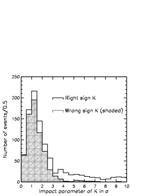
Figure 27: (left) $L/\sigma$ distributions in BTeV for $K^{\pm}$ impact parameters for right sign (unshaded) and wrong sign (shaded) tags. (right) Overall $\epsilon$D² values from kaon tagging for a forward detector containing a flourine based RICH versus a central detector with 100 ns time of flight resolution as a function of kaon impact parameter in units of $L/\sigma$. (Protons have been ignored in both cases.)

The simulation of the central detector gives much poorer numbers. In Fig. 27 (right) $\epsilon D^{2}$ for both the forward and central detectors are shown as a function of the kaon impact parameter (protons have been ignored). It is difficult to get $\epsilon D^{2}$ of more than 1.5% in the central detector.

This analysis shows the importance of detecting protons. Both LHC-B and BTeV are in the process of seeing if low momentum K/p separation can be obtained using another radiator.

5.2.3 Lepton tags

The semileptonic decay process ${B}\to X\ell^{+}{\nu}$ provides, in principle, a excellent way of tagging. The branching ratio to either muons or electrons is large, $\sim$10%. Unfortunately, the process $B\to\overline{D}X^{\prime},\overline{D}\to Y\ell^{-}\bar{\nu}$ produces opposite sign leptons and is hard to separate at hadron colliders. It may be possible to distinguish the charm decay vertex from the $b$ decay vertex in a forward detector, but this has not yet been investigated. Not using this idea, $\epsilon D^{2}$ for muon is 1.5% in the forward detector and 1.0% in the central detector. Electrons are similar, but somewhat worse giving $\epsilon D^{2}$ of 1% in the forward detector.

5.2.4 Jet charge tags

Jet charge is a weighted measure of the charge of the jet producing the tagging $b$. This technique was invented at LEP. It has been successfully used by CDF [38]. They define the jet charge as

$$Q_{jet}={{\Sigma q_{i}\left|\overrightarrow{p_{i}}\cdot\overrightarrow{a}\right|}\over{\Sigma\left|\overrightarrow{p_{i}}\cdot\overrightarrow{a}\right|}},$$ (42)

where the sum is over all particles in the jet cone and $\overrightarrow{a}$ is the jet axis.

5.2.5 Summary of tagging efficiencies

CDF has used their data to measure the tagging efficiencies they now achieve and to project what the expect after detector improvements which are either in progress or which they may propose. Currently CDF does not have any kaon tagging. However, they believe a time-of-flight system would allow them to achieve an $\epsilon D^{2}$ of 3%. BTeV simulations indicate that only 1.5% is possible. Currently CDF measures a same side tagging (SST) efficiency of $(1.5\pm 0.4)$%. They extrapolate to 2% because their new silicon vertex detector will give a cleaner selection of fragmentation tracks. Using jet charge they currently measure ($1.0\pm 0.3$)% and extrapolate to 3%, again due the improved silicon detector.

The tagging efficiency projections are summarized for BTeV and a Central Detector in Table 3. BTeV expects, without proof, that their superior pixel vertex detector will allow even better efficiencies than CDF, but for now uses the CDF projected values. For BTeV $\epsilon D^{2}$ is projected to be larger than 10%. In subsequent simulations 10% will be used.

Table 3: Projected tagging efficiencies ($\epsilon D^{2}$).

	kaon	muon	electron	SST	jet charge	sum
BTeV	5%	1.5%	1.0%	$>$2%	$>$ 3%	$>$10%
Central Detector	0%	1.0%	0.7%	2%	3%	6%

5.3 Measurement of $x_{s}$

BTeV has studied the feasability of measuring the $B_{s}$ mixing parameter $x_{s}$ = $\Delta m_{s}/\Gamma_{s}$. This measurement is key to obtaining the right side of the unitarity triangle shown in Fig. 1. The value of $x_{s}$ may be expected to fall in the range indicated in Fig. 4. This is a large range and demostrates how hard it may be to measure. Recall that for $B_{d}$ mesons, $x$ = 0.73. Thus the oscillation length for $B_{s}$ mixing is at least a factor of 10 shorter and may approach a factor of 100!

Figure 28: Several analysis quantities determined for the $\psi K^{*o}$ final state. $L/\sigma_{L}$ is the distance of the decay from the primary divided by its error; $d_{30}$ refers to the distance of closest approach of the $B$ direction to the primary (projecting backward along the its momentum vector). $\tau$ refers to the lifetime of each event.

BTeV has investigated two final states which can be used. The first $\psi K^{*o}$, $\psi\to\mu^{+}\mu^{-}$ and $K^{*o}\to K^{-}\pi^{+}$ has several advantages. It can be selected using either a dilepton or detached vertex trigger. Backgrounds can be reduced in the analysis by requiring consistency with the $\psi$ and $K^{*o}$ masses. Furthermore, it should have excellent time resolution as there are four tracks coming directly from the $B$ decay vertex. The one disadvantage is that the decays is Cabibbo suppressed, the Cabibbo allowed channel being $\psi\phi$ which is useless for mixing studies. The branching ratio therefore is predicted to have the low value of $8.5\times 10^{-5}$.

Some important analysis quantities and their errors are shown in Fig. 28. The lifetime resolution, $\sigma_{\tau}$ is 45 fs.

BTeV estimates that they will obtain 225 events/“Snowmass year”. (A “Snowmass year has $10^{7}$ seconds.) The signal to background is 3.4:1. This probably could be increased with little loss of efficiency by requiring that no other tracks be consistent with the $B$ decay vertex, but this has not yet been done.

The time distributions of the unmixed and mixed decays are shown in Fig. 29, along with a calculation of the likelihood of there being an oscillation as determined by fits to the time distributions. Background and wrong tags are included.

Figure 29: The observed decay time distributions for $B_{s}\to\psi K^{*o}$ generated with $x_{s}=40$. Unmixed decays are shown in (a), mixed in (b). Background and miss tagging has been included. In (c) the results of a likelihood fit to the time distributions are shown. The dashed line shows a 5$\sigma$ difference from the best solution.

The fitting proceedure correctly finds the input value of $x_{s}=40$. The danger is that a wrong solution will be found. The dashed line shows the change in likelihood corresponding to 5 standard deviations. If our criteria is that the next best solution be greater than $5\sigma$, then this is the best that can be done with one years worth of data in this mode. Once a clean solution is found, the error on $x_{s}$ is quite small, being $\pm 0.15$ in this case.

BTeV has also investigated the $D_{s}^{+}\pi^{-}$ decay of the $\overline{B}_{s}$, with $D_{s}^{+}\to\phi\pi^{+}$. It turns out that the lifetime resolution is 45 fs, the same as for the $\psi K^{*o}$ decay mode. Since the predicted branching ratio for this mode is 0.3%, many more such events are obtainable in one year of running. Fig. 30 shows the $x_{s}$ reach obtainable for a $5\sigma$ discrimination between the favorite solution and the next best solution, for both decay modes. The background is assumed to be 20% and the flavor mistag fraction is taken as 25%. The tagging efficiency is taken as 10%. The dashed lines show the number of years of running, where one year is $10^{7}$ seconds.

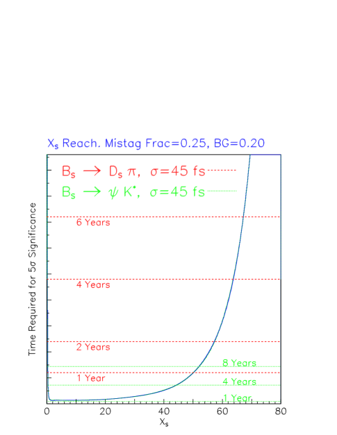
Figure 30: The $x_{s}$ reach for both $D_{s}^{+}\pi^{-}$ and $\psi K^{*o}$ decays of the $\overline{B}_{s}$ The points at which the dashed lines intersect the curve shows the number of years required to make a significant measurement (see text) using $D_{s}\pi$, while the dotted lines show the same thing for $\psi K^{*o}$.

The $x_{s}$ reach is excellent and extends over the entire predicted Standard Model range. The curve gets very steep near $x_{s}$ values of 50 because the time resolution is too poor to resolve the oscillations.

LHC-B has modeled 40 fs resolution in $D_{s}^{+}\pi^{-}$ and will be able to make an excellent measurement of $B_{s}$ mixing.

5.4 Measurement of the CP violating asymmetry in $B^{o}\to\pi^{+}\pi^{-}$

The trigger efficiency for this mode has already been discussed. For the $B^{o}\to\pi^{+}\pi^{-}$ channel BTeV has compared the offline fully reconstructed decay length distributions in their forward geometry with that of detector configured to work in the central region. Fig. 31 shows the normalized decay length expressed in terms of $L/\sigma$ where $L$ is the decay length and $\sigma$ is the error on $L$ for the $B^{o}\to\pi^{+}\pi^{-}$ decay [39].

The forward detector clearly has a much more favorable $L/\sigma$ distribution, which is due to the excellent proper time resolution. Being able to keep high efficiency in the trigger and analysis levels and being able to decimate the backgrounds relies mainly on having the excellent $L/\sigma$ distribution shown for the forward detector.

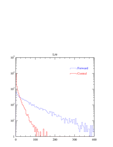
Figure 31: Comparison of the $L/\sigma$ distributions for the decay $B^{o}\to\pi^{+}\pi^{-}$ in central and forward detectors produced at a hadron collider with a center of mass energy of 1.8 TeV.

For this analysis $L/\sigma$ is required to be $>10$. Each pion track is required to miss the primary vertex by a distance/error $>5\sigma$ and that the $B^{o}$ point back to the primary by a distance/error $<2\sigma$. Furthermore, each track is required to be identified as a pion and not a kaon in the RICH detector. Without particle identification it is impossible to distinguish $B^{o}\to\pi^{+}\pi^{-}$ from the combination of $B^{o}\to K^{\pm}\pi^{\mp}$, $B_{s}\to K^{+}K^{-}$ and $B_{s}\to K^{\pm}\pi^{\mp}$, as is shown on Fig. 32. Here $\cal{B}$$(B^{o}\to K^{\pm}\pi^{\mp})$ is taken as $1.5\times 10^{-5}$ and $\cal{B}$$(B^{o}\to\pi^{+}\pi^{-})$ is taken as $0.75\times 10^{-5}$, from recent CLEO measurements [41]. The $B_{s}$ decay into $K^{+}K^{-}$ is assumed to have the same rate as the $B^{o}$ decay into $K^{\pm}\pi^{\mp}$, and the $B_{s}$ decay into $K^{\pm}\pi^{\mp}$ is assumed to have the same rate as the $B^{o}$ decay into $\pi^{+}\pi^{-}$.

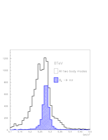
Figure 32: Invariant mass distributions of all $B\to h^{+}h^{-}$ final states, where $h$ denotes either a pion or kaon, and the mass is computed assuming that both tracks are pions. The plot on the left shows the individual background channels and the one on the right shows the sum of all channels properly normalized (see text) to the $\pi^{+}\pi^{-}$ signal.

Using the good particle identification, BTeV predicts that they can measure the CP violating asymmetry in $\pi^{+}\pi^{-}$ to $\pm 0.05$ as detailed in Table 5.4.

2cmlccQuantity Value

Cross-section 100 $\mu$b

Luminosity $0.5\times 10^{32}$

# of $B^{o}$/Snowmass year $3.8\times 10^{8}$

$\cal{B}$$(B^{o}\to\pi^{+}\pi^{-})$ $0.75\times 10{-5}$

Reconstruction efficiency 0.09

Triggering efficiency (after all other cuts) 0.72

# of $\pi^{+}\pi^{-}$ 17000

$\epsilon D^{2}$ for flavor tags ($K^{\pm}$, $\ell^{\pm}$, same + opposite sign jet tags) 0.1

# of tagged $\pi^{+}\pi^{-}$ 1700

Signal/Background 0.4

Error in asymmetry (including background) $\pm 0.05$

Table 4: Numbers entering into the accuracy in measuring the CP violating asymmetry in $B^{o}\to\pi^{+}\pi^{-}$.

5.5 Finding the rare decay $B^{-}\to K^{-}\mu^{+}\mu^{-}$

Interesting rare decays include dimuon, dielectron and single photon channels. The rates are largest among the single photon channels. However, the feasability of trigger and analyzing these decays has not been attempted. The branching ratios are larger for muons than electrons. They are given in Table 5 [42].

Table 5: Rare dimuon decay branching ratios.

channel	$B^{-}\to K^{-}\mu^{+}\mu^{-}$	$\overline{B}^{o}\to K^{*o}\mu^{+}\mu^{-}$	$B^{-}\to\mu^{+}\mu^{-}$	$B_{s}\to\phi\mu^{+}\mu^{-}$	$B_{s}\to\mu^{+}\mu^{-}$
predicted $\cal{B}$	$4\times 10^{-7}$	$1.5\times 10^{-6}$	$1.5\times 10^{-10}$	$1.5\times 10^{-6}$	$3.5\times 10^{-9}$

The final state we are discussing has a significantly lower branching ratio than available in $B_{s}\to\phi\mu^{+}\mu^{-}$. Furthermore, the narrow $\phi$ is useful for background suppression. Thus this mode should be easier to detect.

While tagging is not needed for this physics, the backgrounds are a problem. To detect these rare final states, a veto must be put on final states which are decays of the $\psi$ or $\psi^{\prime}$, which are much more prolific. Similar cuts are applied as used when studying $B^{o}\to\pi^{+}\pi^{-}$. It is interesting to note that requiring kaon identification in the RICH reduces the background by a factor of three without significantly reducing the efficiency. These events can be triggered on either the detached vertex or the dimuon lines. The analyis efficiency is 2.5% and the trigger efficiency on events which pass the analysis cuts is 85%. BTeV finds 300 signal events using an integrated luminosity of 500 pb^-1 with a signal to background of 0.4.

6 Comparisons

6.1 Comparison with $e^{+}e^{-}$ $B$ factories

Let us compare one example of the physics reach of a foward collider detector (BTeV) with $e^{+}e^{-}$ $B$ factories operating at the $\Upsilon$(4S). Table 6 shows the effective number of flavor tagged $B^{o}\to\pi^{+}\pi^{-}$ events found in a Snowmass year of running. The branching ratio is assumed to be $0.75\times 10^{-5}$.

Table 6: Number of tagged $B^{o}\to\pi^{+}\pi^{-}$

	$\cal{L}$(cm-2s-1)	$\sigma$	#$B^{o}/10^{7}$s	efficiency	$\epsilon D^{2}$	# tagged
$e^{+}e^{-}$	$3\times 10^{33}$	1 nb	$3.0\times 10^{7}$	0.4	0.4	46
BTeV	$5\times 10^{31}$	100 $\mu$b	$3.5\times 10^{10}$	0.065	0.1	1700

Clearly the hadron collider experiment has the ability to collect far more events.

6.2 Comparison of BTeV with Tevatron central detector

There are several important areas where BTeV has crucial advantages over a Tevatron central detector.

• The detached vertex trigger.- The ability to trigger on decay verticies allows BTeV to address important issues in charm physics including mixing and CP violation. It allows accumulation of a plethora of interesting $B$ decay states including semileptonic decays and hadronic decays such as $B^{o}\to\pi^{+}\pi^{-}$ and $\overline{B}_{s}^{o}\to D_{s}^{+}h^{-}.$

• Resolution on detached vertex.- The $L/\sigma_{L}$ distribution as shown in Fig. 31 is much more favorable for the forward detectors. This allows for high efficiency for detecting the final state of interest and permits good background rejection.

• Charged hadron identification.- Crucial for measurement of many final states and CP asymmetries. For example, determining the CP asymmetries in $B^{o}\to\pi^{+}\pi^{-}$, $B_{s}\to K^{+}K^{-}$, $B_{s}\to D_{s}^{\pm}K^{\mp}$. It also provides a larege increase in flavor tagging efficiency which helps to precisely measure all asymmetries.

6.3 Comparison of LHC-B with BTeV

There are issues favoring both LHC-B and BTeV:

• Issues favoring LHC-B

  • The $b$ cross-section is expected to be five times larger at LHC than at the Tevatron.

  • The mean number of interactions per beam crossing is four times lower at LHC than at the Tevatron even when the bunch spacing at FNAL is 132 ns.

• Issues favoring BTeV

  • BTeV is a two-arm spectrometer which increases the physics yield by a factor of two relative to LHC-B.

  • The 25 ns bunch spacing at LHC makes first level detached vertex triggering more difficult than at the Tevatron with 132 ns bunch spacing.

  • The seven times larger LHC beam energy causes problems. There is a much larger range of track momentua that need to be momentum analyzed and identified, and there is a large increase in track multiplicity which causes difficulties in triggering and pattern recognition.

  • BTeV is designed with the vertex detector in the magnetic field in order to reject low momentum tracks at the trigger level. Low momentum tracks can multiple scatter and cause false triggers.

  • The detached vertex trigger in BTeV allows for charm physics studies.

7 Conclusions

The BTeV and LHC-B programs, emphasizing studies of mixing, CP violation and rare decays offer exciting and unique physics opportunities prior to (BTeV) and in the LHC era (BTeV and LHC-B). Standard Model parameters will be precisely measured and physics beyond the Standard Model may appear.

Acknowledgments

I would like to thank my BTeV colleagues including Marina Artuso, Joel Butler, Chuck Brown, Paul Lebrun, Patty McBride, Mike Procario and Tomasz Skwarnicki for their help in getting this material together. This work was supported by the U. S. National Science Foundation.

References

References

- [1] P. Rankin, at this school.
- [2] P. Roudeau at this school.
- [3] F. Bedeschi at this school.
- [4] F. Abe et al, Phys. Rev. Lett. 75, 1451 (1995); S. Abachi et al., Phys. Rev. Lett. 74, 3548 (1995).
- [5] S. Frixione, M.L. Mangano, P. Nason, and G. Ridolfi Nucl.Phys. B431, 453(1994) and references contained therein.
- [6] For more information on BTeV see http://fnsimu1.fnal.gov/btev.html
- [7] For more information on LHC-B see http://wwwlhcb.cern.ch/
- [8] N. Cabibbo, Phys. Rev. Lett. 10, 531 (1963); M. Kobayashi and K. Maskawa, Prog. Theor. Phys. 49, 652 (1973).
- [9] L. Wolfenstein, Phys. Rev. Lett. 51, 1945 (1983). The imaginary term occurs in order in and . The term in is important for CP violation in decay.
- [10] M. Gaillard and B. Lee, Phys. Rev. D10, 897, (1974); J. Hagelin, Phys. Rev. D20, 2893, (1979); A. Ali and A. Aydin, Nucl. Phys. B148, 165 (1979); T. Brown and S. Pakvasa, Phys. Rev. D31, 1661, (1985); S. Pakvasa, Phys. Rev. D28, 2915, (1985); I. Bigi and A. Sanda, Phys. Rev. D29, 1393, (1984).
- [11] H. Albrecht et al, Phys. Lett. B192, 245 (1983).
- [12] Using the ratio of like-sign to opposite sign dilepton events, UA1 published a mixing signal at the 3 level that resulted from a combination of and , see C. Albajar et al, Phys. Lett B186, 245 (1987).
- [13] T. Bowcock, R. Hawkings, G. Passaleva and C. Zeitnitz, Nucl. Instrum. Methods A384, 48 (1996).
- [14] A. J. Buras, “Theoretical Review of B-physics,” in BEAUTY ’95 ed. N. Harnew and P. E. Schlein, Nucl. Instrum. Methods A368, 1 (1995).
- [15] The CESR B Physics Working Group, K. Lingel et al, “Physics Rationale For a B Factory”, Cornell Preprint CLNS 91-1043 (1991); SLAC Preprint SLAC-372 (1991); “Progress Report on Physics and Detector at KEK Asymmetric B Factory,” KEK Report 92-3 (1992)
- [16] S. Stone, “Prospects For B-Physics In The Next Decade,” presented at NATO Advanced Study Institute on Techniques and Concepts of High Energy Physics, Virgin Islands, July 1996, to be published in procedings.
- [17] The first papers explaining the phyiscs of mixing and CP violation in decays were A. Carter and A. I. Sanda, Phys. Rev. Lett. 45, 952 (1980); Phys. Rev. D23, 1567 (1981); I. I. Bigi and A. I. Sanda, Nucl. Phys. B193, 85 (1981); ibid B281, 41 (1987).
- [18] P. Langacker, “CP Violation and Cosmology,” in CP Violation, ed. C. Jarlskog, World Scientific, Singapore p 552 (1989).
- [19] D. Atwood, I. Dunietz and A. Soni, Phys. Rev. Lett. 78, 3257 (1997).
- [20] Private communication from I. Bigi and G. Burdman.
- [21] M. Golden and B. Grinstein Phys. Lett. B 222, 501 (1989); F. Buccella et al, Phys. Rev. D 51, 3478 (1995).
- [22] The reader is referred to an excellent series of workshops organized by P. Schlein. The most recent proceedings are published in F. Ferroni and P. E. Schlein, Nucl. Instrum. Methods A384, 1 (1996).
- [23] M. Gronau and D. London, Phys. Rev. Lett. 65, 3381 (1990); N.G. Deshpande, X-G. He, and S. Oh, Phys. Lett. B 384, 283 (1996); A. Buras and R. Fleischer, Phys. Lett. B 360, 138 (1995); M. Gronau and J. L. Rosner, Phys. Lett. B 76, 1200 (1996); A. S. Dighe, M. Gronau, and J. L. Rosner, Phys. Rev. D 54, 3309 (1996); A. S. Dighe and J. L. Rosner, Phys. Rev. D 54, 4677 (1996). R. Fleischer and T. Mannel, Phys. Lett. B 397, 269 (1997); C. S. Kim, D. London and T. Yoshikawa, “Using Decays to Determine the CP Angles and , hep-ph/9708356 UdeM-GPP-TH-97-43 (1997).
- [24] M. Beneke, G. Buchalla, I. Dunietz, Phys. Rev. D 54, 4419 (1996).
- [25] R. Aleksan, B. Kayser and D. London, “In Pursuit of ,” DAPNIA/SPP 93-23, NSF-PT-93-4, UdeM-LPN-TH-93-184, hep-ph/9312338 (1993); R. Aleksan, I. Dunietz and B. Kayser, Z. Phys. C 54, 653 (1992).
- [26] M. Artuso, “Experimental Facilities for b-Quark Physics,” in Decays revised 2nd Edition, Ed. S. Stone, World Scientific, Sinagapore (1994).
- [27] F. Abe et al, Phys. Rev. D 53, 1051 (1996).
- [28] M. Mangano, P. Nason and G. Ridolfi, Nucl. Phys. B 373, 295 (1992).
- [29] F. Abe et al, Phys. Rev. Lett. 75, 1451 (1995). Previous UA1 measurements agreed with the theoretical predictions, see C. Albajar et al, Phys. Lett. B 256, 121 (1991). Recent D0 measurements agree with both the CDF measurements and the high side of the theoretically allowed range. See S. Abachi et al, Phys. Rev. Lett. 74, 3548 (1995).
- [30] J. Ellet et al, Nucl. Instr. and Meth. A317 28, (1992).
- [31] G. Wilkinson, Nucl. Instrum. Methods A 368, 169 (1995); the trigger is undergoing revisions.
- [32] R. Desalvo, Nucl. Instrum. Methods A 384, 153 (1996).
- [33] R. Forty, CERN-PPE/96-176, Sept. 1996 published in Proc. of the Int. Workshop on physics at Hadron Machines, Rome, Italy, June 1996, F. Ferroni, P. Schlein (Eds.), North-Holland, 1996.
- [34] “LHC-B Letter of Intent,” CERN/LHCC 95-5, LHCC/18 (1995), which can be viewed at http://www.cern.ch/LHC-B/loi/loi_old.html .
- [35] P. Avery et al, “MCFast: A Fast Simulation Package for Detector Design Studies,” Presented at The International Conference on Computing in High Energy Physics, Berlin 1997. To appear in the proceedings.
- [36] V. M. Marzulli, Nucl. Instrum. Methods A 384, 237 (1996).
- [37] These results are based on the work of R. Isik, W. Selove, and K. Sterner,“Monte Carlo Results for a Seconday-vertex Trigger with On-line Tracking,” Univ. of Penn. preprint UPR-234E (1996).
- [38] W. Yao, “Tagging Strategies,” presented at “Workshop on Heavy Quark Physics at C-Zero,” Fermilab (1996).
- [39] M. Procario, “ Physics Prospects beyond the Year 2000,” invited talk at 10th Topical Workshop on Proton-Antiproton Physics, Fermilab-CONF-95/166 (1995).
- [40] P. McBride and S. Stone, Nucl. Instr. and Meth. A368, 38 (1995).
- [41] CLEO Collaboration, “Observation of Exclusive Rare Charmless Decays,” CONF 97-24, eps97-334 (1997).
- [42] N. G. Deshpande, “Theory of Penguins in Decays,” in Decays revised 2nd edition, ed. S. Stone, World Scientific, Singapore (1994).