Abstract

We present an overview of the research activities of the theoretical particle physics group at the University of Mainz on the calculation of massive one- and two-loop Feynman diagrams. The main objective of this research was to develop an automatic one- and two-loop calculation program package. A first version of such a program was recently realized by Brücher, Franzkowski and Kreimer. We describe in some detail the present features of this automatic loop calculation program as well as the integration techniques that go into the program. The program runs under the name of XLOOPS. The present version is labelled by XLOOPS 1.0. The program allows one to calculate massive one- and two-loop integrals in the Standard Model including their tensor structure - all at the click of a mouse. Renormalization features are included in that the UV divergences in UV divergent integrals are explicitly computed in dimensional regularization. One-loop integrals are calculated analytically in $d\neq 4$ dimensions whereas two-loop integrals are reduced to two-fold integral representations which the program evaluates numerically. We attempt to provide a synopsis of the novel loop integration techniques that have been developed for the XLOOPS program. They allow for a fast and efficient evaluation of massive one- and two-loop integrals. We discuss Higgs decay at the two-loop level as a first application of the novel integration techniques that are incorporated into XLOOPS .

1 Introduction

In the last few years a large part of the theoretical particle physics group at the University of Mainz has been involved in the computation of massive one- and two-loop Feynman integrals. This activity was part of a continuing group seminar series on the evaluation of Feynman diagrams. Apart from the work of the senior members of the group many beautiful new results have been achieved by our diploma and PhD students in the context of their thesis work. Present members of the group are L. Brücher, M. Fischer, J. Franzkowski, A. Frink, S. Groote, V. Kleinschmidt, J.G. Körner, R. Kreckel, D. Kreimer, A.J. Leyva, M. Mauser, K. Schilcher and J.B. Tausk. Past members of the group include A. Czarnecki, U. Kilian, K. Melnikov, D. Pirjol, P. Post and O. Yakovlev. We have greatly benefitted from the many visitors and guest scientists who have visited our group over the years and who have generously shared with us their insights into the calculational techniques of Feynman diagram computations. They are too numerous to be all quoted here in name. All of this effort would not have been possible without the support of various funding agencies. These include the DFG (Deutsche Forschungsgemeinschaft) with individual grants as well as stipends provided by the Graduiertenkolleg “Teilchenphysik bei hohen und mittleren Energien”, the BMBF (Bundesministerium für Bildung und Forschung) and a HUCAM project granted by the European Union.

This write-up is certainly in the character of a workshop write-up. We take this opportunity to present an overview of the activities of our group and the results obtained therein. In particular this means that we do not attempt to give a balanced account of the present state of art of loop calculations the world over. We ask for forebearness. It is clear that the results that we are presenting are too numerous to have been obtained by any single person alone. The results represent the efforts of various subsets of the members of the group. When discussing particular results we shall not always specify the subset of members of the group that were involved in a particular calculation in order to avoid excessive cross-referencing. The respective members can be identified from the references.

By means of introduction we want to remark that there are two main approaches to doing loop calculations. The one approach we would like to call the absorptive-dispersive approach. One first calculates the absorptive parts of a Feynman diagram and then uses dispersion relations with possible subtractions to obtain the dispersive part of the Feynman diagram. The experience is that the absorptive-dispersive approach usually goes further when calculating two-loop diagrams if the aim is to perform analytically as many of the necessary integrations as possible. This is particularly true for two-loop diagrams with internal loop masses.

There are many examples of two-loop calculations that have been done using the absorptive-dispersive integration technique. For example, in Mainz we have calculated the two-loop gauge boson contributions to the decay $H\rightarrow\gamma+\gamma$ using the absorptive-dispersive technique [1]. The calculations were done using the Equivalence Theorem. In the high energy limit the transition $H\rightarrow\gamma+\gamma$ is dominated by the longitudinal degrees of freedom of the internal loop gauge bosons which can be represented by the massless and spinless Goldstone excitations of an effective scalar theory. The Higgs boson is the only massive particle in the theory. It appears both as external and internal loop particle. There are a number of two-loop diagrams that contribute to the process. They are too numerous to be all shown here. All absorptive contributions were determined analytically, and all but one of the remaining dispersive integrals were done analytically. In Fig.1

Figure 1: Three-particle cut of a crossed ladder diagram contributing to $H\to\gamma+\gamma$. Solid lines: mass Higgs particles; dashed lines: massless gauge bosons of the effective theory.

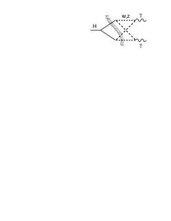
we show the contribution of the three-particle cut of the the massive two-loop crossed ladder three-point function which was the only contribution which did not yield to analytical integration in the dispersion integral. The remaining one-dimensional dispersion integral of this one particular contribution was then done numerically. One of the outcomes of the analysis was that the results of the effective theory should be reliable in the range $0.6\,\mbox{TeV}\leq m_{H}\leq 1.5\,\mbox{TeV}$. Above $1.5\,\mbox{TeV}$ the two-loop result blows up.

In another example the absorptive-dispersive approach was used to calculate the two-loop contributions to the $K^{0}$ charge radius in chiral perturbation theory [2]. Quite naturally the loop masses in chiral perturbation theory cannot be neglected since chiral perturbation theory is an effective low energy theory. The final result of the calculation was obtained in terms of a one-dimensional integral representation which was evaluated numerically.

As a curious side remark we want to emphasize that it is even sometimes advantageous to take the opposite route and first calculate the full loop contribution directly and then extract its imaginary part. For example, rate calculations can be done quite efficiently in this way. If one shies away from phase-space integrations but knows how to do loop calculations e.g. by Feynman parameter methods then one can obtain rates very efficiently from the imaginary part of the full loop contribution. This technique has been used to great advantage in the calculation of the inclusive semileptonic differential rate of polarized $\Lambda_{b}$’s to polarized $\tau$’s within the Operator Expansion method in HQET [3]. The relevant one-loop diagram is shown in Fig.2 together with its absorptive cut which determines the rate of the decay.

Figure 2: Rate of $\Lambda_{b}^{(\uparrow)}\to X_{c}+\tau^{-(\uparrow)}+\bar{\nu}_{\tau}$ extracted from the absorptive part of the one-loop amplitude $\tau^{+(\uparrow)}+\Lambda_{b}^{(\uparrow)}\to\tau^{+(\uparrow)}+\Lambda_{b}^{(\uparrow)}$ .

A large part of the remaining discussion in this presentation will concern itself with the direct computation of massive two-loop integrals not using the absorptive-dispersive approach. As a general feature of the direct approach we shall find that all but two of the massive two-loop integrations can be done analytically. In the absorptive-dispersive approach there are many examples where one can go further and where all but one of the massive two-loop calculations can be done analytically. A noteworthy example is the efficient one-dimensional integral representation written down by Bauberger and Böhm for the general massive two-loop two-point function [4]. This has to be compared with the two-fold integral representation derived in the direct approach to be discussed later on. However, the absorptive-dispersive approach involves a detailed consideration of the two- and three-particle cut structure of the contributing diagrams including possible subtraction terms and anomalous threshold contributions which is not always simple theoretically. In particular the requisite analysis does not possess the flexibility which is needed for a general purpose program package that we were aiming for.

2 Direct Approach to Loop Calculations

In Mainz we have developed a completely new approach to the calculation of massive one- and two-loop diagrams. These radically new integration techniques have been devised in a series of ingenious papers by Kreimer [5, 6, 7, 8]. In order to appreciate the quality of innovation of these new techniques let us briefly recapitulate the main features of the more traditional approach to loop integrations. The essential integration features employed by most practitioners in the field may be summarized by the following statements

• integrate covariantly

• introduce a set of Feynman parameters

• perform a Wick rotation and integrate in Euclidean space

• do tensor integrals à la Passarino-Veltman

In comparison to the above program the Mainz method may be characterized by the following list of statements

• integrate in a special frame (usually the rest frame of one of the external particles)

• no Feynman parameters

• do the integrations in Minkowski space

• tensor integrals are worked out by direct integration

The traditional integration methods become progressively more intractable when more and more mass scales are introduced into a problem. This has led many authors to introduce quite radical approximations such as setting the ratios $m_{W}/m_{t}$ and $m_{Z}/m_{t}$ to zero in their loop calculations without being able to say much about the error invoked by such an approximation. Contrary to this the Mainz integration methods are ideally suited for the most general mass case with as many different massive loop particles as possible. In fact Standard Model calculations with $m_{t}\neq m_{W}\neq m_{Z}\neq m_{H}$ are quite welcome. In the other extreme one generally has no problems taking the mass zero limit in a loop contribution if the diagram does not contain any infrared (IR) or mass (M) singularities. In the presence of IR/M singularities the corresponding integrals have to be regularized by subtraction as will be discussed later on.

In order to provide a measure of the scope of what XLOOPS [9] can do at the moment and what XLOOPS hopes to be able to do in the future we have drawn a representative set of loop diagrams in Fig.3 which are labelled as: A1 (two-point one-loop), A2 (two-point two-loop), B1 (three-point one-loop), B2 (three-point two-loop), C1 (four-point one-loop) and C2 (four-point two-loop). In Table 1 we list the status of these loop calculations as concerns their availability in the present version XLOOPS 1.0 and, if not implemented in XLOOPS 1.0, we comment on their stage of development.

loop class	status and availability
2-point 1-loop	XLOOPS 1.0
2-point 2-loop	XLOOPS 1.0
3-point 1-loop	XLOOPS 1.0
	UV divergences : ready
3-point 2-loop	IR/M divergences : starting
	tensor structure : conceptually ready
4-point 1-loop	ready for implementation
4-point 2-loop	starting

Table 1: Present status of one- and two-loop calculations in XLOOPS

Figure 3: Representative set of diagrams to be treated in XLOOPS

3 Parallel and orthogonal momentum space

A very important technical concept in our loop calculations is the splitting of total $d$-dimensional space into a parallel space spanned by the external momenta and an orthogonal space spanned by its orthogonal complement. Symbolically we write

total space = parallel($\parallel$) space + orthogonal($\perp$) space

The orthogonal space components of the loop momenta have no orientation in the real world defined by parallel space. For scalar integrals this implies a spherical symmetry in orthogonal space which can be nicely exploited. Tensor integrals involving orthogonal components can easily be evaluated since their expansion along resultant tensors involves only combinations of orthogonal space metric tensors. These can be easily processed further. Also, by splitting $\gamma$-matrices into their orthogonal and parallel space components almost all the tedious $\gamma$-matrix algebra in fermionic amplitudes can be avoided.

Let us illustrate the advantages of working in orthogonal space with the help of a few examples. We begin with the two-point function with any number of loops as drawn in symbolic fashion in Fig.4.

Figure 4: Two-point function with any number of loops

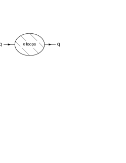
The external momentum and thus parallel space is defined by the momentum $q_{\mu}$. The dimensionality of the two respective spaces is thus given by

parallel space $(\parallel)$	:	1-dimensional
orthogonal space $(\perp)$	:	$(d-1)$-dimensional

The metric tensor $g_{\mu\nu}$ splits up into a parallel piece $g_{\mu\nu}^{\parallel}$ and a orthogonal piece $g_{\mu\nu}^{\perp}$ according to $g_{\mu\nu}=g_{\mu\nu}^{\parallel}+g_{\mu\nu}^{\perp}$. The respective components of the metric tensor can easily be constructed, $viz$.

$$g_{\mu\nu}^{\parallel} = q_{\mu}q_{\nu}/q^{2}$$ (1)

$$g_{\mu\nu}^{\perp} = g_{\mu\nu}-q_{\mu}q_{\nu}/q^{2}$$ (2)

Quite naturally the two components of the metric tensor can be used to project out the parallel and orthogonal components of any $d$-dimensional vector.

In a similar way one can split up the $\gamma$-matrix into its parallel and orthogonal components according to

$$\gamma_{\mu}=\gamma_{\mu}^{\parallel}+\gamma_{\mu}^{\perp}$$ (3)

By using the metric projectors it is easy to see that one has $\gamma_{\mu}^{\parallel}=q\kern-5.5pt/q_{\mu}/q^{2}$ and $\gamma_{\mu}^{\perp}=\gamma_{\mu}-q\kern-5.5pt/q_{\mu}/q^{2}$. Note also that $\gamma_{\mu}^{\parallel}$ and $\gamma_{\mu}^{\perp}$ anticommute, i.e. one has

$$\left[\gamma_{\mu}^{\parallel},\gamma_{\nu}^{\perp}\right]_{+}=0$$ (4)

The anticommutativity of the two respective $\gamma$-matrix components results in an extremely expedient way of dealing with the $\gamma$-matrix algebra when evaluating fermionic Feynman diagrams. We shall return to this point later on.

In the case of the $n$-loop three-point function one has two independent external momenta $q$ and $p$ that define parallel space. A symbolic representation of the $n$-loop three-point function is drawn in Fig.5.

Figure 5: Three-point function with any number of loops

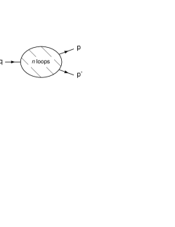
Assuming that the momentum $q$ is time-like one chooses the rest frame of $q$ as the reference frame (if $q$ is space-like one chooses the rest frame of one of the other momenta). In this frame the momenta $q$ and $p$ are represented by $q=(q^{0},0,0,0)$ and $p=(p_{0},p_{z},0,0)$ such that the three-momentum $\vec{p}$ defines the $z$-direction in parallel space. The dimensions of the two respective spaces is now given by

parallel space $(\parallel)$	:	2-dimensional
orthogonal space $(\perp)$	:	$(d-2)$-dimensional

As before the metric tensor splits into the the two components

$$g_{\mu\nu}=g_{\mu\nu}^{\parallel}+g_{\mu\nu}^{\perp}$$ (5)

where one has

$$g_{\mu\nu}^{\parallel}=\frac{1}{q^{2}}q_{\mu}q_{\nu}-\frac{1}{p_{z}^{2}}\left(p_{\mu}p_{\nu}-\frac{(pq)^{2}}{q^{4}}q_{\mu}q_{\nu}\right)$$ (6)

and $g_{\mu\nu}^{\perp}$ is given by the complement $g_{\mu\nu}-g_{\mu\nu}^{\parallel}$.

We briefly side-track to remind the reader that the construction of a parallel and an orthogonal space is a familiar concept used also in other areas of particle physics even if different names are attached to the two respective spaces. For example, one talks of the longitudinal and transverse component of a four-vector current $J_{\mu}$ with respect to its momentum $q$. The transverse component $J_{\mu}^{\perp}$ is then defined through the relation $q^{\mu}J_{\mu}^{\perp}=0$. In a similar vein in HQET one chooses a time-like four-velocity $v_{\mu}$ with $v^{2}=1$ which serves to define longitudinal and transverse components of a general four-vector $a_{\mu}$ according to $a_{\mu}^{\parallel}=a\cdot vv_{\mu}$ and $a_{\mu}^{\perp}=a_{\mu}-a\cdot vv_{\mu}$. In the dynamical formulation of HQET this splitting up of four-dimensional space-time becomes an important dynamical concept in as much as the covariant derivative $D_{\mu}$ is split up into its longitudinal piece $D_{\mu}^{\parallel}=D\cdot vv_{\mu}$ and its transverse piece $D_{\mu}^{\perp}=D_{\mu}-D\cdot vv_{\mu}$. In the $v$ rest frame $v_{\mu}=(1,0,0,0)$ the longitudinal and transvere covariant derivatives reduce to the time-derivative $D_{0}$ and the three-derivative $\vec{D}$, respectively. The $1/m_{Q}$ expansion of the theory must then be organized in such a way that in the rest frame of $v$ higher order derivatives involve only the three-derivative $\vec{D}$ whereas the time-derivative $D_{0}$ must appear only to first order [10].

In the two examples discussed before (two- and three-point function) orthogonal space was $(d-1)$- and $(d-2)$-dimensional. The continuation of space-time away from $d=4$ facilitates the regularization of ultraviolet (UV) and IR/M singularities. All one-loop calculations in XLOOPS are in fact carried out in $d\neq 4$ dimensions in order to be able to control the UV and IR/M divergences. As it turns out the two-loop integrations cannot be done in $d\neq 4$ dimensions in the generality that is needed for the implementation in XLOOPS. Instead the divergent pieces of the integrands are first identified. One then subtracts and adds auxiliary integrand functions that have the same degree of divergence but which are sufficiently simple to allow for their integration in $d\neq 4$ dimensions. The divergent behaviour of the original integrand is thereby eradicated such that its numerical integration can be performed in $d=4$ dimensions. The divergent auxiliary function is then integrated using dimensional regularisation to the required accuracy in powers of $\varepsilon=(d-4)/2$.

In the UV case the auxiliary integrand functions are constructed from the same Feynman diagram which the auxiliary integrand functions are sought to reproduce in their UV behaviour, however, with some of the momenta and masses in the diagram set to zero. It is clear that one has to be careful to avoid introducing spurious IR/M divergences in the course of this procedure. The construction of the requisite auxiliary integrand functions has been fully automated and is implemented in XLOOPS.

If a diagram contains IR/M divergences one proceeds in a similar fashion. However, the construction of the requisite auxiliary integrand functions is not as simple as in the UV case. As of yet we have not been able to solve the problem of constructing the auxiliary integrand functions in all generality. There is a certain amount of progress, though, in that we have been able to demonstrate the feasibility of this approach for some specific and important cases. The two cases treated so far are the two-loop $O(\alpha_{s}^{2})$ contributions to the $b\rightarrow c$ transition at zero recoil and the two-loop contributions to $Z\rightarrow b\bar{b}$.

There are altogether 13 two-loop contributions to the transition $b\rightarrow c$. According to the Lee-Nauenberg theorem the sum of the 13 two-loop contributions are IR finite at zero recoil because the accompanying Bremsstrahlung diagrams are kinematically suppressed at this point and can therefore not be called upon for IR cancellation. But taken separately single diagrams generally do have IR singularities which have to be regularized. The requisite set of auxiliary integrand functions have been explicitly constructed. After subtraction the remaining IR finite contributions were integrated analytically. We mention that the corresponding one-loop calculation had been done in the early 80’s for any value of the momentum transfer variable [11]. The first complete analytical zero recoil two-loop calculation was published this year by Czarnecki and Melnikov[12, 13].

Figure 6: Parallel ladder two-loop diagram contributing to $Z\to b\bar{b}$.

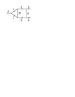
The second example concerns the determination of the $O(g^{2}\alpha_{s})$ mixed electroweak and QCD two-loop contributions to $Z\rightarrow b\bar{b}$. These radiative corrections are important for high precision tests of the Standard Model. In Fig.6 we show one of the contributing diagrams which is of “parallel ladder” type. In our first exploratory calculation we neglected spin effects and calculated only the scalar parallel ladder diagram. The diagram is IR divergent, and, for $m_{b}=0$, also M divergent. The IR/M behaviour of this diagram and a few other parallel ladder diagrams was improved in the manner described above. The remaining IR/M finite integration was computed numerically using the two-fold integral representation of massive two-loop contributions which is also available in XLOOPS. The auxiliary integrand functions were then integrated in $d\neq 4$ dimensions obtaining its IR/M divergent piece as well as its finite contribution. In order to check on the results of this numerical evaluation the contribution of the same diagram was then calculated using completely different integration methods, namely the improved small momentum expansion method developed in Refs.[14]. The numerical results were compared and satisfactory agreement was found [15].

For the remaining part of this presentation we presume that the UV and IR/M improvement program for the integrands has been carried through such that there is no need for regularization. The remaining discussion will be centered around integration methods in $d=4$ dimensions.

4 Tensor integrals and strings of $\gamma$-matrices

In order to illustrate the advantages of using parallel/orthogonal space techniques we return to the two-loop two-point case. In Fig.7

Figure 7: Two-loop two-point function: the master topology

we have drawn the generic diagram of the so called master topology which is the most difficult diagram in the two-loop two-point category. Included are also the flow of the loop momenta $l$ and $k$. The propagator line $3$ contains both loop momenta $l$ and $k$ and will therefore be referred to as mixed propagator line. The other propagator lines $1,2$ and $4,5$ contain only one loop momentum, namely $l$ and $k$, respectively. Assuming that $q$ is time-like, the diagram is evaluated in the $q$-rest frame where $q^{\mu}=(q^{0},0,0,0)$. (If $q$ is space-like the corresponding contribution can be obtained by analytic continuation from the time-like region.) The loop momenta split up into their parallel and orthogonal space components according to $l^{\mu}=(l^{0},\vec{l}_{\perp})$ and $k^{\mu}=(k^{0},\vec{k}_{\perp})$.

Assume now that there is a $\gamma$-matrix string associated with the diagram. Remembering that parallel and orthogonal $\gamma$-matrices mutually anticommute and that they anticommute with $\gamma_{5}$ the string can always be arranged into pieces of the form

$$\gamma_{5}^{n_{5}}\gamma_{0}^{n_{0}}\vec{\gamma}^{\perp}\ldots\vec{\gamma}^{\perp}$$ (7)

where the $n_{5}$ $\gamma_{5}$’s have been moved to the left end of the string and the $n_{0}$ $\gamma_{0}$’s to second to left. The products of $\gamma_{5}$’s and $\gamma_{0}$’s can then be simplified by using $\gamma_{5}^{2}=1$ and $\gamma_{0}^{2}=1$. If one has an even string of $\vec{\gamma}^{\perp}$-matrices the string of $\vec{\gamma}^{\perp}$-matrices can be replaced by products of orthogonal space metric tensors whose weights are determined by the trace of the $\vec{\gamma}^{\perp}$-matrices. For those $\vec{\gamma}^{\perp}$-matrices that are contracted with the orthogonal space loop momenta $\vec{l}_{\perp}$ and $\vec{k}_{\perp}$ an appropriate symmetrization has to be carried out w.r.t. multiply occurring loop momentum indices. That is, returning to the covariant description, one has the replacement

$$\gamma_{\mu_{1}}^{\perp}\ldots\gamma_{\mu_{n}}^{\perp}\Rightarrow g_{{\mu_{1}}{\mu_{2}}}^{\perp}\ldots g_{{\mu_{n-1}}{\mu_{n}}}^{\perp}+\ldots+\mbox{symmetrization}$$ (8)

Odd strings of $\vec{\gamma}^{\perp}$-matrices can be seen to give zero results after integration. The case that the two-loop two-point master diagram carries external tensor indices will not be discussed further here but similar simplifications on the $\gamma$-matrix algebra can be seen to occur.

Returning to Eq.(7) the Dirac-string object $/\kern-4.0ptl/\kern-6.0ptk$ can be replaced by $l_{0}k_{0}-\vec{l}_{\perp}\cdot\vec{k}_{\perp}$. The orthogonal space scalar product $\vec{l}_{\perp}\cdot\vec{k}_{\perp}$ contains the cosine of the polar angle between $\vec{l}_{\perp}$ and $\vec{k}_{\perp}$. For further processing it is advantageous to get rid of the polar angle dependence through cancellation with the mixed propagator $P_{3}=(l+k)^{2}-m_{3}^{2}$. This can be achieved by writing

$$\vec{l}_{\perp}\cdot\vec{k}_{\perp}=\hbox{$\frac{1}{2}\ $}(l_{0}^{2}+k_{0}^{2}-\vec{l}_{\perp}^{2}-\vec{k}_{\perp}^{2}-m_{3}^{2}+2l_{0}k_{0}-P_{3})$$ (9)

The mixed propagator factor $P_{3}$ cancels against the corresponding denominator factor and one remains with a factorizable two-loop contribution. The other terms are genuine two-loop contributions. However, they no longer possess a $\cos\theta$ dependence in the integrand numerator. They can therefore be further processed as in the scalar case to be discussed in the next section.

If there are external indices attached to a diagram one has to solve the problem of how the loop contributions distribute themselves onto the various covariants that determine the covariance structure of the diagram. Again this problem is solved very elegantly using parallel/orthogonal space techniques. As an illustration we choose the simple example of the two-point function carrying two external Lorentz indices corresponding to the self-energy of an off-shell boson. The covariance structure of the resulting contribution has the form $C_{1}g_{\mu\nu}+C_{2}q_{\mu}q_{\nu}$. The invariant $C_{1}$ can be picked out by calculating the orthogonal component of the two-loop integral since $q_{\mu}q_{\nu}$ has no orthogonal space component. After having calculated $C_{1}$ the invariant $C_{2}$ can then be obtained by considering the parallel space component of the two-loop integral. In the language of contractions the invariant $C_{1}$ is obtained by contraction with $g^{\mu\nu}_{\perp}$ since $q_{\mu}q_{\nu}g^{\mu\nu}_{\perp}=0$. Once $C_{1}$ is known the invariant $C_{2}$ can be obtained by contraction with the parallel space tensor $q_{\mu}q_{\nu}$. Admittedly the example that we have discussed is of a rather simple nature but it still serves to illustrate the important point that the parallel/orthogonal space method allows one to efficiently evaluate tensor loop integrals. Much of the tedious algebra of matrix inversions needed in the Passarino-Veltman method of calculating tensor integrals is avoided since the use of parallel/orthogonal space techniques lead to an almost complete diagonalization of the problem from the outset.

5 The two-loop two-point function:
the master diagram

Here we give a brief review of the derivation of Kreimer’s two-dimensional integral representation [5] for the scalar master diagram (see Fig. 7). This is mainly intended to be a warming-up exercise before we discuss the non-planar three-point function in the next section.

The master diagram depends on one external momentum, $q$, and five masses $m_{i}$, $(i=1,\ldots,5)$. In the scalar case, it is UV-finite, and can therefore be calculated in $d=4$ without any subtractions:

$$I\;=\;I(q^{2};m_{1},\ldots,m_{5})\;=\;\int\int\mbox{d}^{4}k\;\mbox{d}^{4}l\;\frac{1}{P_{1}P_{2}P_{3}P_{4}P_{5}}\;,$$ (10)

where

$$P_{1} = {l}^{2}-m_{1}^{2}+i\rho$$

$$P_{2} = {(l-q)}^{2}-m_{2}^{2}+i\rho$$

$$P_{3} = {(k+l)}^{2}-m_{3}^{2}+i\rho$$

$$P_{4} = {k}^{2}-m_{4}^{2}+i\rho$$

$$P_{5} = {(k+q)}^{2}-m_{5}^{2}+i\rho\;.$$ (11)

For the time being we shall assume that the external momentum is time-like $(q^{2}>0)$, so that we can work in its rest frame, in which $q=(q_{0},\vec{0})$, $k=(k_{0},\vec{k}_{\perp})$ and $l=(l_{0},\vec{l}_{\perp})$. Introducing $k_{\perp}=|\vec{k}_{\perp}|$, $l_{\perp}=|\vec{l}_{\perp}|$ and the polar angle $\theta$ between $\vec{k}_{\perp}$ and $\vec{l}_{\perp}$, we rewrite the propagators as

$$P_{1}=\omega_{1}^{2}-l_{\perp}^{2}, \omega_{1}=\sqrt{l_{0}^{2}-m_{1}^{2}+i\rho}$$

$$P_{2}=\omega_{2}^{2}-l_{\perp}^{2}, \omega_{2}=\sqrt{(l_{0}-q_{0})^{2}-m_{2}^{2}+i\rho}$$

$$P_{3}=\omega_{3}^{2}-k_{\perp}^{2}-l_{\perp}^{2}-2k_{\perp}l_{\perp}\cos\theta, \omega_{3}=\sqrt{(k_{0}+l_{0})^{2}-m_{3}^{2}+i\rho}$$

$$P_{4}=\omega_{4}^{2}-k_{\perp}^{2}, \omega_{4}=\sqrt{k_{0}^{2}-m_{4}^{2}+i\rho}$$

$$P_{5}=\omega_{5}^{2}-k_{\perp}^{2}, \omega_{5}=\sqrt{(k_{0}+q_{0})^{2}-m_{5}^{2}+i\rho}.$$ (12)

The important points to note here are that only the mixed propagator, $P_{3}$, depends on $\theta$, and that the differences $P_{1}-P_{2}$ and $P_{4}-P_{5}$ only depend on the parallel space variables $k_{0}$ and $l_{0}$. After performing three trivial angular integrations, the integral (10) becomes

$$I = 8\pi^{2}\int_{-\infty}^{\infty}\mbox{d}k_{0}\int_{-\infty}^{\infty}\mbox{d}l_{0}\;\frac{1}{(P_{1}-P_{2})(P_{4}-P_{5})}\int_{0}^{\infty}k_{\perp}^{2}\,\mbox{d}k_{\perp}\int_{0}^{\infty}l_{\perp}^{2}\,\mbox{d}l_{\perp}$$ (13)

$$\times \int_{-1}^{1}\mbox{d}\cos\theta\left(\frac{1}{P_{1}P_{3}P_{4}}-\frac{1}{P_{1}P_{3}P_{5}}+\frac{1}{P_{2}P_{3}P_{5}}-\frac{1}{P_{2}P_{3}P_{4}}\right).$$

Let us concentrate on the first term in the parantheses on the second line of Eq. (13). The integral over the orthogonal space variables can be regarded as a vacuum integral with “masses” $\omega_{1}$, $\omega_{3}$, $\omega_{4}$ in $d=3$. The $z$ integral is elementary:

$$\int_{0}^{\infty}k_{\perp}^{2}\,\mbox{d}k_{\perp}\int_{0}^{\infty}l_{\perp}^{2}\,\mbox{d}l_{\perp}\frac{1}{P_{1}P_{4}}\int_{-1}^{1}\mbox{d}\cos\theta\frac{1}{P_{3}}$$ (14)

$$= \int_{0}^{\infty}k_{\perp}^{2}\,\mbox{d}k_{\perp}\int_{0}^{\infty}l_{\perp}^{2}\,\mbox{d}l_{\perp}\frac{1}{P_{1}P_{4}}\frac{1}{2k_{\perp}l_{\perp}}\log\left[\frac{(l_{\perp}-k_{\perp})^{2}-\omega_{3}^{2}}{(l_{\perp}+k_{\perp})^{2}-\omega_{3}^{2}}\right]$$

$$= -\frac{1}{2}\int_{-\infty}^{\infty}\mbox{d}k_{\perp}\int_{-\infty}^{\infty}\mbox{d}l_{\perp}\frac{k_{\perp}l_{\perp}}{(l_{\perp}^{2}-\omega_{1}^{2})(k_{\perp}^{2}-\omega_{4}^{2})}\log\left[l_{\perp}+k_{\perp}+\omega_{3}\right]\,.$$

Now, both the $k_{\perp}$ and $l_{\perp}$ integrations can be performed by closing the integration contours in the complex plane (taking care not to cross the cut of the logarithm) and applying Cauchy’s theorem, which gives:

$$-\frac{(2\pi i)^{2}}{8}\log\left[\omega_{1}+\omega_{3}+\omega_{4}\right].$$ (15)

Collecting the four terms in (13) and expressing everything in terms of the dimensionless variables $x=l_{0}/q_{0}$, $y=k_{0}/q_{0}$, we finally obtain:

$$I=\frac{4\pi^{4}}{q^{2}}\int_{-\infty}^{\infty}\mbox{d}x\int_{-\infty}^{\infty}\mbox{d}y\;\frac{1}{w_{1}^{2}-w_{2}^{2}}\frac{1}{w_{4}^{2}-w_{5}^{2}}\log\left[\frac{(w_{1}+w_{3}+w_{4})(w_{2}+w_{3}+w_{5})}{(w_{2}+w_{3}+w_{4})(w_{1}+w_{3}+w_{5})}\right]$$ (16)

with

$$w_{1}=\sqrt{x^{2}-\frac{m_{1}^{2}}{q^{2}}+i\rho} w_{2}=\sqrt{(x-1)^{2}-\frac{m_{2}^{2}}{q^{2}}+i\rho}$$

$$w_{3}=\sqrt{(x+y)^{2}-\frac{m_{3}^{2}}{q^{2}}+i\rho} w_{4}=\sqrt{y^{2}-\frac{m_{4}^{2}}{q^{2}}+i\rho}$$

$$w_{5}=\sqrt{(y+1)^{2}-\frac{m_{5}^{2}}{q^{2}}+i\rho}.$$ (17)

The representation (16) is valid for arbitrary masses, and it gives the correct analytic continuation to space-like external momenta. Except for a few very special threshold configurations, it is possible to take the limit $\rho\to 0$ under the integral sign, yielding an integrand which is continuous in the entire $(x,y)$ plane and can easily be integrated numerically. An attractive feature of this result is that we do not have to distinguish whether $q^{2}$ is below, in between, or above the thresholds: one simple formula covers all cases. Eq.(16) also gives the correct imaginary part.

Tensor integrals (of rank greater than one) require subtractions to make them UV-convergent. XLOOPS automatically performs the necessary subtractions [8] and then generates two-dimensional numerical integrands for the finite remainders that are very similar to the one derived here for the scalar case. The only difference is that they contain additional factors of $x$, $y$, or $w_{i}$ in the numerator which are not difficult to deal with.

6 The two-loop three-point function:
the crossed ladder configuration

Starting from the two-point master topology, one obtains the crossed ladder topology by attaching the third leg to the central propagator, as shown in Fig.8. This is the most complicated two-loop three-point topology because, no matter how the loop momenta $k$ and $l$ are routed, one cannot avoid having two mixed propagators that depend on the scalar product $k\cdot l$. Another way of drawing this topology is shown in Fig.11.

Figure 8: The two-loop crossed vertex diagram

In this section, we will give a brief and somewhat simplified account of how a two-fold integral representation for this diagram can be obtained. For a more detailed explanation, and for other two-loop three-point topologies, we refer to [16, 9].

The scalar integral is defined by

$$V\;=\;V(q_{1}^{2},q_{2}^{2},q^{2};m_{1},\ldots,m_{6})\;=\;\int\int\mbox{d}^{4}k\;\mbox{d}^{4}l\;\frac{1}{P_{1}P_{2}P_{3}P_{4}P_{5}P_{6}}\;,$$ (18)

where $q=q_{1}+q_{2}$ and the propagators are

$$P_{1} = {(k+l-q_{1})}^{2}-m_{1}^{2}+i\rho$$

$$P_{2} = {(k+l+q_{2})}^{2}-m_{2}^{2}+i\rho$$

$$P_{3} = {(l-q_{1})}^{2}-m_{3}^{2}+i\rho$$

$$P_{4} = {(k+q_{2})}^{2}-m_{4}^{2}+i\rho$$

$$P_{5} = {l}^{2}-m_{5}^{2}+i\rho$$

$$P_{6} = {k}^{2}-m_{6}^{2}+i\rho\;.$$ (19)

We use a frame where $q=(e_{1}+e_{2},0,\vec{0})$, $q_{1}=(e_{1},q_{z},\vec{0})$, $q_{2}=(e_{2},-q_{z},\vec{0})$, $k=(k_{0},k_{1},\vec{k}_{\perp})$ and $l=(l_{0},l_{1},\vec{l}_{\perp})$. This time, $\vec{k}_{\perp}$ and $\vec{l}_{\perp}$ are two-component vectors. Introducing polar coordinates in the orthogonal space and carrying out one trivial angular integration, we find that

$$\int\mbox{d}^{4}k\;\int\mbox{d}^{4}l\ldots$$ (20)

$$= 2\pi\int_{-\infty}^{\infty}\mbox{d}k_{0}\int_{-\infty}^{\infty}\mbox{d}l_{0}\;\int_{-\infty}^{\infty}\mbox{d}k_{1}\;\int_{-\infty}^{\infty}\mbox{d}l_{1}\;\int_{0}^{\infty}k_{\perp}\,\mbox{d}k_{\perp}\int_{0}^{\infty}l_{\perp}\,\mbox{d}l_{\perp}\int_{0}^{2\pi}\mbox{d}\theta\ldots$$

$$= \frac{\pi}{2}\int_{-\infty}^{\infty}\mbox{d}\tilde{k}_{0}\int_{-\infty}^{\infty}\mbox{d}\tilde{l}_{0}\;\int_{0}^{\infty}\mbox{d}s\int_{0}^{\infty}\mbox{d}t\int_{-\infty}^{\infty}\mbox{d}k_{1}\;\int_{-\infty}^{\infty}\mbox{d}l_{1}\;\int_{0}^{2\pi}\mbox{d}\theta\ldots\,,$$

where $s=l_{\perp}^{2}$ and $t=k_{\perp}^{2}$. In the last line, we have replaced $k_{0}$ and $l_{0}$ with the shifted variables $\tilde{k}_{0}=k_{0}-k_{1}$ and $\tilde{l}_{0}=l_{0}-l_{1}$. As a result, all the propagators become linear in $k_{1}$ and $l_{1}$, e.g.

$$P_{6}=k_{0}^{2}-k_{1}^{2}-t-m_{6}^{2}+i\rho=\tilde{k}_{0}^{2}+2\tilde{k}_{0}k_{1}-t-m_{6}^{2}+i\rho\,.$$ (21)

Thus, the $k_{1}$ and $l_{1}$ integrations can be performed by closing the contours in either the upper or lower half plane and applying Cauchy’s theorem. In order to understand the general structure of the result of using Cauchy’s theorem, let us decompose the integral into $(2\times 2\times 2=8)$ partial fractions of the form

$$\int_{-\infty}^{\infty}\mbox{d}k_{1}\;\int_{-\infty}^{\infty}\mbox{d}l_{1}\;\frac{1}{(k_{1}-z_{1})(l_{1}-z_{2})(k_{1}+l_{1}+z_{3})}=\frac{(2\pi i)^{2}}{z_{1}+z_{2}+z_{3}}.$$ (22)

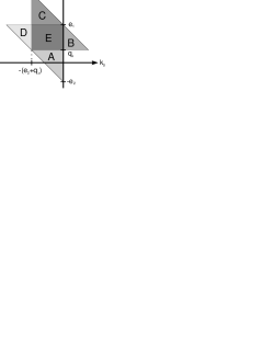
This equation holds when the signs of the imaginary parts of $z_{1}$, $z_{2}$ and $z_{3}$ are all equal. Otherwise, the integral on the left hand side vanishes. Now the imaginary parts of the $z_{i}$’s all come from the infinitesimal $i\rho$, divided by linear combinations of $\tilde{k}_{0}$, $\tilde{l}_{0}$ and the external momenta (cf. eg. eq. (21)). As a consequence, each term of the partial fraction decomposition only gives a non-vanishing contribution inside a finite, triangular region in the $(\tilde{k}_{0},\tilde{l}_{0})$ plane. The union of those triangles is shown in Fig. 9.

After a further partial fraction decomposition wrt. $\cos\theta$, the $\theta$-integration can be carried out using

$$\int_{0}^{2\pi}\mbox{d}\theta\frac{1}{A-B\cos\theta}=\frac{2\pi}{\sqrt{A^{2}-B^{2}}}$$ (23)

(and being careful to pick the correct branch of the square root on the right hand side!).

Having performed the $k_{1}$, $l_{1}$ and $\theta$ integrations, one obtains the following intermediate expression:

$$V\;=\;\sum_{j}\frac{C_{j}\theta_{j}}{\sqrt{(a_{j}t+b_{j}+c_{j}s)^{2}-4st}}\prod_{i=1}^{3}\frac{1}{(\tilde{a}_{ij}t+\tilde{b}_{ij}+\tilde{c}_{ij}s)}\,.$$ (24)

The quantities $C_{j}$, $a_{j}$, $b_{j}$, $c_{j}$, $\tilde{a}_{ij}$, $\tilde{b}_{ij}$ and $\tilde{c}_{ij}$ are all rational functions of $\tilde{k}_{0}$, $\tilde{l}_{0}$, $q_{i}$ and $m_{i}$. $\theta_{j}$ is a product of step functions restricting $\tilde{k}_{0}$ and $\tilde{l}_{0}$ to one of the triangles discussed above.

By means of Euler’s change of variables, it is possible to get rid of the square root in (24) and perform both the $s$ and $t$ integrals analytically, leading, eventually, to dilogarithms and Clausen functions. Although the final expression is too long to be listed here in explicit form, it is a sufficiently well-behaved function to allow the remaining $\tilde{k}_{0}$ and $\tilde{l}_{0}$ integrations to be evaluated numerically without problems.

Figure 9: Integration region in the $(\tilde{k}_{0},\tilde{l}_{0})$ plane

7 Checks on two-loop three-point functions

We have performed a number of checks on the integration methods that go into XLOOPS as well as on the performance of XLOOPS itself. Some of these checks have been discussed before, as e.g. checks on the two-loop $O(\alpha_{s}^{2})$ contributions to the $b\rightarrow c$ transition at zero recoil.

As concerns the two-loop three-point function the checks divide up into checks on the correctness of the theoretical structure of the results and numerical cross-checks against the results of other authors for specific mass cases. For example, we have checked that the two-fold integral representations of the parallel and crossed ladder contributions have the

• correct cut structure in the analytic plane as prescribed by the Landau-Cutkosky cutting rules

• possess the correct anomalous threshold behaviour at the prescribed anomalous thresholds

We have looked at all two-particle cuts and, with particular care, at all three-particle cuts and have found that the analyticity structure of our parallel and crossed ladder two-loop results are in complete agreement with the Landau-Cutkosky cutting rules.

As a check on the correct anomalous threshold behaviour we ran our numerical program across an anomalous threshold. We start with the one-loop vertex contribution which possesses anomalous thresholds at

$$1+2\mu_{1}\mu_{2}\mu_{3}-\mu_{1}^{2}-\mu_{2}^{2}-\mu_{3}^{2}=0$$ (25)

where ($i=1,2,3$)

$$\mu_{i}=\frac{(m_{1}^{2}+m_{2}^{2}+m_{3}^{2}-m_{i}^{2}-p_{i}^{2})m_{i}}{2m_{1}m_{2}m_{3}}$$ (26)

As sample values we took the following set of masses and momenta (in arbitrary units)

$$m_{1}=m_{2}=m_{3}=1$$ (27)

$$p_{1}^{2}=6,\,p_{2}^{2}=5,\,p_{3}^{2}=-4-\sqrt{15}\approx-7.873$$ (28)

$$\begin{array}[]{cc}\psfig{width=78.04842pt}&\psfig{width=78.04842pt}\\ \psfig{width=173.44534pt}&\psfig{width=173.44534pt}\\ {\scriptstyle{\sf p_{3}^{2}}}&{\scriptstyle{\sf p_{3}^{2}}}\end{array}$$

Figure 10: Plot of real and imaginary parts of a vertex function in the vicinity of an anomalous threshold, one-loop (left) and two-loop (right)

In Fig.10 we show the values of the imaginary and the real partof the vertex contribution in the vicinity of the anomalous threshold at $p_{3}^{2}\approx-7.873$. The plot clearly shows the logarithmic type singularity of an anomalous threshold at $x=x_{0}$ which reads

$$i\ln(x-x_{0})+C(x)=i\ln|x-x_{0}|\,\pm\,\pi\theta(x-x_{0})+C(x)$$ (29)

where $C(x)$ is a complex-valued function that is regular in the vicinity of $x=x_{0}$. We also checked on the anomalous threshold behaviour of the corresponding parallel ladder two-loop vertex correction. The two-loop vertex correction has an anomalous threshold at the same position $p_{3}^{2}\approx-7.873$ for any values of the masses $m_{4},m_{5},m_{6}$. The numerical evaluation of the two-loop graph showed the same behaviour around the anomalous threshold as the one-loop graph (see Fig.10). The numerical stability in the direct vicinity of the anomalous threshold was found to be satisfactory in both cases but was somewhat decreased in the two-loop case relative to the one-loop case.

Further we ran our program for specific mass configurations and compared the numerical results with the results of other groups. For example, we evaluated the crossed ladder vertex graph for external momenta with $q^{2}=p_{1}^{2}=p_{2}^{2}\neq 0$ and let the internal masses $m_{i}=m(i=1,\ldots,6)$ go to zero. When $m=0$ Ussyukina and Davydychev have shown that the crossed ladder configuration can be calculated analytically, and that the result turns out to be equal to the square of a one-loop graph [17]. Our numerical $m\rightarrow 0$ results agree with the Ussyukina-Davydychev limit. It came as a pleasant surprise that numerical stability was retained in this limit.

Next we took the specific momentum configuration $p_{1}^{2}=p_{2}^{2}=0$ and set all six internal masses in the crossed ladder configuration to $m=150$ GeV. We compared our results with the corresponding calculation by Tarasov [18], who used an improved small momentum expansion using conformal mapping and Padé approximants. There was full agreement on the real and imaginary parts of the crossed ladder configuration above, below and close to threshold $q^{2}=4m^{2}$. In particular there was no noticeable decline in numerical stability close to threshold which had been a troublesome region in the low momentum expansion method before it was improved by conformal mapping. It is not so simple to compare the time performance of the two approaches since the low momentum expansion method requires a great amount of preparatory work in that the coefficients of the low momentum expansion have to be calculated first.

We also compared our results to an evaluation of the crossed ladder contribution to $Z(\mbox{off-shell})\rightarrow t\bar{t}$ done by the Japanese KEK group Fujimoto et al.[19]. The relevant mass configuration

Figure 11: Crossed ladder two-loop contribution to $Z(\mbox{off-shell})\rightarrow t\bar{t}$.

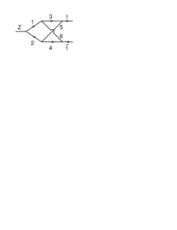
is $m_{1}=m_{2}=m_{3}=m_{4}=\sqrt{q_{1}^{2}}=\sqrt{q_{2}^{2}}=150$ GeV (the would-be mass of the top quark in 1994) and $m_{5}=m_{6}=91$ GeV. The contribution clearly corresponds to the off-shell $Zt\bar{t}$ vertex with internal $Z$ and $t$ exchange. Again we found full numerical agreement for both the real and imaginary parts. The Japanese group used Feynman parametrization and reduced the number of necessary numerical loop integrations to three by analytic integration. For comparable accuracy the necessary computing time is considerably smaller in the Mainz approach.

As a final example of the reliability of the massive two-loop crossed and parallel ladder integration techniques and the numerical integration techniques based on them we discuss a recent application of these methods to the calculation of the dominant two-loop corrections, of order ${\cal O}(G_{F}^{2}M_{H}^{4})$, to the partial widths of the decays of a heavy Higgs to pairs of W- and Z-bosons, carried out in collaboration with B.A. Kniehl and K. Riesselmann [20]. The calculation was done again using the Equivalence Theorem, i.e. the dominant longitudinal degrees of freedom of the gauge bosons were represented by the massless and spinless Goldstone boson excitations of the effective theory. Of the many contributing diagrams we show only two representative diagrams of the class of crossed and parallel ladder configurations which are the most difficult to calculate.

Figure 12: Two-loop parallel and crossed ladder contributions to $H\to ZZ$ in the effective theory. Solid lines: massive Higgs particles; dashed lines: massless gauge bosons.

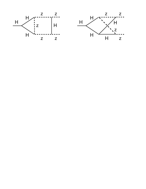
In the numerical evaluation of these diagrams we started off with small finite Goldstone masses which were then set to smaller and smaller values and finally to zero. We found that the numerical results were stable in this limit. After compounding the contributions of the many contributing diagrams and carrying out the renormalization in the on-shell scheme, the correction factor was found to be $1+14.6\%(m_{H}/\mbox{TeV})^{2}+16.9\%(m_{H}/\mbox{TeV})^{4}$, indicating that for $m_{H}>1\mbox{TeV}$ the Standard Model ceases to be weakly interacting. Numerically, this result agrees with that of Ghinculov, who had used entirely different integration techniques to evaluate the same decay process [21]. From the fact that the calculation involves a large number of massive two-loop diagrams that contribute to the process we believe that the numerical agreement of the two calculations provides for another strong test of the reliability of our integration techniques and the numerical routines based on them as well as those used by Ghinculov. We mention that a two-loop calculation of the fermionic contributions to $H\to ZZ,WW$ is under way.

8 Some sample calculations with XLOOPS

This summer saw the première of a live performance of XLOOPS during a talk given by J. Franzkowski at the Klausurtagung of the Mainz Graduiertenkolleg “Teilchenphysik bei hohen und mittleren Energien”. For the performance he used a laptop and a projectable screen display. Nothing can beat the excitement of a live performance of XLOOPS either at a PC session or during a talk using a projector screen. We shall nevertheless try to capture some of the spirit of a live demonstration of XLOOPS by presenting two sample calculations done by XLOOPS. In the first example we calculate the on-shell one-loop self-energy of the neutral gauge boson $Z$ resulting from the contribution of the top quark loop. In the second example we calculate one of the mixed $O(g^{2}\alpha_{s})$ QCD/electroweak contributions to the two-loop flavour-changing self-energy of the $s\rightarrow d$ quarks.

Figure 13: XLOOPS display of a one-loop Feynman diagram.

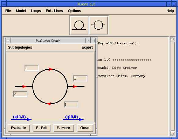
At the beginning of an XLOOPS session one has to specify the model whose Feynman rules are to be used in the loop evaluation. In both of the examples to be discussed here one clicks on “Standard Model” in the “Model” menu which would call up the Feynman rules of the Standard Model. Also the user has to specify the numbers $m$ and $n$ for his choice of the $m$-point $n$-loop function. In the case of the one-loop self-energy of the $Z$ he would then click on “two” external lines ($m=2$) and on “one” loop ($n=1$). The topology bar would then show the two possible two-point one-loop topologies. These can be discerned at the top of Fig.13. One then clicks on the desired topology which would be the second of the two topologies in Fig.13. After having selected the topology the desired one-loop graph appears on the screen in an enlarged version as shown in Fig.13.

One then has to attach arrows to the lines in the graph according to the quantum number flow (wrongly pointed arrows would lead to an error message) and specify the particles in the graph by inserting the particle names in the particle entry fields. In the next step one has to specify the mass and momentum parameters. There is an “Insert Particle Properties” option as a menu entry which automatically substitutes the mass values provided by the latest version of the Particle Data Group listings. Mass values can of course also be introduced by hand. In our example we have $m_{Z}=91.187$ GeV and $m_{t}=176$ GeV. The one-loop graph is evaluated in the rest system of the on-shell $Z$. Thus one chooses $q_{10}=91.187$ GeV. The calculation of the graph is then executed by clicking on the “E.(Evaluate)Full” bar. In this one-loop example the numerical answer would appear within seconds in the following format:

[

C1 = [

                                                  -16
 146.22583756233107509 I, .26077710144029877423*10    - 1219.7690445131992210 I

 ],

C2 = [.00096061186286253340551 I,

                            -20
    .18797591473406467665*10    - .0080036871858407297497 I],

C1 G(nu1, nu2) + C2 q1(nu1) q1(nu2)]

The numerical output is given in terms of the two invariants $C_{1}$ and $C_{2}$ in the covariant expansion $C_{1}g_{\mu\nu}+C_{2}q_{\mu}q_{\nu}$. Each of the invariants is displayed as a list $[a,b]$ which represents a series $a/\varepsilon+b+{\cal O}(\varepsilon)$. In the present case the coefficients $a$ are purely imaginary while the $b$’s have a tiny real part, that would vanish if the causal $i\rho$’s in the propagators were put to zero exactly. This corresponds to the fact that in the present momentum configuration, below the $t\bar{t}$-threshold, the self-energy $\Sigma$ (which differs from the diagram itself by a factor of $i$) is purely real.

Figure 14: XLOOPS input panel for the two-loop master diagram.

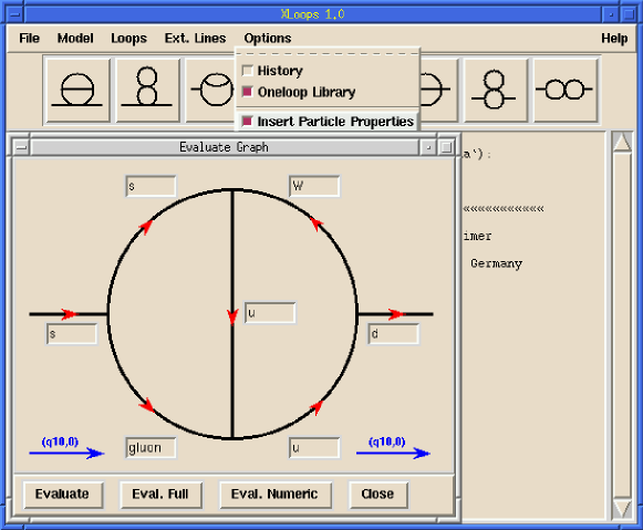
The second example is drawn from a recent determination of the $O(g^{2}\alpha_{s})$ two-loop contribution to the flavour changing self-energy for $s\rightarrow d$. Of the contributing diagrams we take one of the diagrams with a master topology as drawn in Fig.14. One proceeds as was described in the first example only that one specifies to “two” in the menu “Loops”. One recognizes some of the relevant two-loop topologies at the top of the display depicted in Fig.14. In the present example one clicks on the master topology which is the fourth two-loop diagram from the left in the topology bar which is covered up in the display Fig.14. The relevant Feynman diagram pops up in which the quantum number flows and particle names have to be inserted as shown in Fig.14. Finally, after specifying the particle masses and the momentum of the external particle one initiates the numerical evaluation of the diagram:

                                      -6
    [C1 = [ - .68103432226158921830*10   I delta3(tmu1, tmu2),

                                 -5
         .42790442626661980279*10   delta3(tmu1, tmu2)

                                        -5
              - .40233768346700174054*10   I delta3(tmu1, tmu2),

         [%1, [ - 4.98962 - 2.43436 I, .0015744 + .00190137 I]],

         .000026216132920579719619 delta3(tmu1, tmu2)

                                        -6
              + .60792896861672700256*10   I delta3(tmu1, tmu2)],

                                         -6
        C2 = [ - .68103432226158921830*10   I delta3(tmu1, tmu2),

                                    -5
            .42790442626661980279*10   delta3(tmu1, tmu2)

                                           -5
                 - .40233768346700174054*10   I delta3(tmu1, tmu2),

            [%1, [ - 4.99119 - 2.43249 I, .00176832 + .00185428 I]],

            .000026216121704383664719 delta3(tmu1, tmu2)

                                           -6
                 + .59969113686867746914*10   I delta3(tmu1, tmu2)],

        C3 = [.00015525369186016884013 I delta3(tmu1, tmu2),

             - .00051268542153584540755 delta3(tmu1, tmu2)

                 + .00072319063843461738822 I delta3(tmu1, tmu2),

            [%1, [ - 845.404 - 954.737 I, .742148 + .926344 I]],

            3.5949563175956949478 delta3(tmu1, tmu2)

                 + 96495.670995961263803 I delta3(tmu1, tmu2)],

        C4 = [.00015525369186016884013 I delta3(tmu1, tmu2),

             - .00051266860707202340491 delta3(tmu1, tmu2)

                 + .00072847640460045290512 I delta3(tmu1, tmu2),

            [%1, [ - 844.468 - 954.961 I, .576421 + .882752 I]],

            10.877778389998066059 delta3(tmu1, tmu2)

                 + 103995.51572482192447 I delta3(tmu1, tmu2)],

        C1 (1 &* ONE) + C2 (1 &* Dg5) + C3 (1 &* Dg0) + C4 &*(1, Dg5, Dg0)]

                                        -6
%1 :=           .85129290282698652282*10   delta3(tmu1, tmu2)

The results are given in terms of the four invariants $C_{1}$, $C_{2}$, $C_{3}$ and $C_{4}$ in the rest frame decomposition $C_{1}\bar{u}u+C_{2}\bar{u}\gamma_{5}u+C_{3}\bar{u}\gamma_{0}u+C_{4}\bar{u}\gamma_{5}\gamma_{0}u$. For each of the invariants $C_{j}$, the data are shown as a list $[a,b,[c,[d,e]],f]$. Their meaning is as follows: $C_{j}=a/\varepsilon^{2}+b/\varepsilon+c\times(d\pm e)+f+{\cal O}(\varepsilon)$. $f$ is the piece of the finite part of $C_{j}$ that is calculated analytically, $d$ is the part that is obtained by numerical integration, and $e$ is an estimate of the accuracy of the numerical integration. The overall colour factor of the diagram delta3(tmu1, tmu2) is displayed separately. It is calculated from the rules of the $SU(N)$ colour algebra which are known to XLOOPS.

Figure 15: List of four-point two-loop topologies.

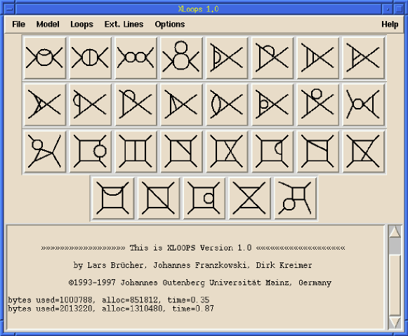
As indicated in Fig.3 and Table 1 we have started work on massive four-point two-loop functions. As a preparatory step we have classified all the two-loop topologies and generated their diagrams. All the four-point two-loop topologies are shown in Fig.15. We shall refer to the $p$-th diagram in the $q$-th row by $(p,q)$. The calculation of diagram $(2,4)$ was done first because of its implication for a two-loop chiral perturbation theory calculation of $\gamma+\gamma\rightarrow\pi+\pi$. The calculation of the scalar diagram $(2,4)$ was recently completed. The techniques of parallel and orthogonal space integrations used in the four-point case are similar to the three-point two-loop case only that parallel space is now 3-dimensional. Six of the eight needed integrations were done analytically. The remaining two-fold integral representation was found to be suitable for numerical processing. The calculation of diagrams $(3,3)$ and $(7,3)$ is well under way.

9 Present status of XLOOPS and outlook

The presently available version of XLOOPS is a demonstration version which runs under the name of XLOOPS 0.9. It is meant to whet the appetite of the user. The demo version features all Standard Model Feynman rules including QCD. It allows one to calculate one-loop graphs up to and including three-point functions. It is available at the web-site http://wwwthep.physik.uni-mainz.de/$\sim$xloops.

A full version XLOOPS 1.0 has been completed and is currently being tested. It is accompanied by a 110 page manual which can be obtained at the above web-site. XLOOPS 1.0 and the manual should be available in a few weeks time. There are some additional features as Feynman rules for the two Higgs doublet model. One of the future items of XLOOPS is the automatic generation of Feynman diagrams from a given set of Feynman rules. One would then like to avail of subsets of the Standard Model Feynman rules. This feature is already incorporated in XLOOPS 1.0 in that one can select the Feynman rules of QED and QCD. XLOOPS 1.0 incorporates first two-loop features in the form of two-loop two-point functions including their tensor decomposition.

As time goes on more features will be added to XLOOPS. We plan to issue XLOOPS 1.1 by the end of this year. It will contain a one-loop four-point function routine including tensor structure capabilitiies. Also XLOOPS 1.1 will be able to automatically generate all one- and two-loop Feynman diagrams that contribute to a given process including a drawing routine which generates Postscript output. Also we plan to install a plotting routine that will generate plots when input parameter values of masses or momenta are varied continuously over a range of the input parameter values. There are also plans to write a longer review on the theoretical background with a detailed description of the calculational techniques that go into XLOOPS .

Work is going on on the two-loop three-point function which is ready conceptually. More Feynman rules will be added such as those of the minimal supersymmetric Standard Model and chiral perturbation theory. Further in the future lies the implementation of the two-loop four-point function which is presently under study. Also we plan to install automatic renormalization capabilities. The ground is prepared for renormalization in that the one-loop routines calculate to $O(\varepsilon)$ accuracy such that one-loop counter terms can be computed automatically. In the very far future we hope to provide the possibility to evaluate complete processes including phase space integration routines for tree graph contributions. All of this needs a great deal of man power. We hope that we can count on the support of the community in this enterprise.

References

- [1] J.G. Körner, K. Melnikov and O.I. Yakovlev, Phys.Rev. D53 (1996) 3737.
- [2] P. Post and J.B. Tausk, Mod. Phys. Lett. A11 (1996) 2115; P. Post and K. Schilcher, hep-ph/9701422, to be published in Phys.Rev.Lett.
- [3] S. Balk, J.G. Körner and D. Pirjol, hep-ph/9703344, to be published in Z. Phys. C.
- [4] S. Bauberger and M. Böhm, Nucl. Phys. B445 (1995) 25.
- [5] D. Kreimer, Phys. Lett. B273 (1991) 277.
- [6] D. Kreimer, Z. Phys. C54 (1992) 667; D. Kreimer, Int. J. Mod. Phys. A8 (1993) 1797; L. Brücher, J. Franzkowski and D. Kreimer, Mod. Phys. Lett. A9 (1994) 2335.
- [7] D. Kreimer, Phys. Lett. B292 (1992) 341; D. Kreimer, Phys. Lett. B347 (1995) 107.
- [8] D. Kreimer, Mod. Phys. Lett. A9 (1994) 1105.
- [9] L. Brücher, J. Franzkowski, A. Frink and D. Kreimer, Nucl. Instrum. Meth. A389 (1997) 323; J. Franzkowski, PhD. Thesis, Mainz, 1997.
- [10] J.G. Körner and G. Thompson, Phys. Lett. B264 (1991) 185; S. Balk, J.G. Körner and D. Pirjol, Nucl. Phys. B428 (1994) 499; B. Holstein, Am. J. Phys. 65 (1997) 519.
- [11] K. Schilcher, Minh D. Tran and N.F. Nasrallah, Nucl. Phys. B181 (1981) 91, E: B187 (1981) 594; J.E. Paschalis and G.J. Gounaris, Nucl. Phys. B222 (1983) 473.
- [12] A. Czarnecki, Phys.Rev.Lett. 76 (1996) 4124.
- [13] A. Czarnecki and K. Melnikov, Karlsruhe preprint TTP97-08 (hep-ph/9703277).
- [14] D.J. Broadhurst, J. Fleischer and O.V. Tarasov, Z. Phys. C60 (1993) 287 ; J. Fleischer and O.V. Tarasov, Z. Phys. C64 (1994) 413; F.A. Berends, A.I. Davydychev, V.A. Smirnov and J.B. Tausk, Nucl. Phys. B439 (1995) 536; J. Fleischer, V.A. Smirnov and O.V. Tarasov, Z. Phys. C74 (1997) 379.
- [15] J. Fleischer, A. Frink, J.G. Körner, D. Kreimer, K. Schilcher, V.A. Smirnov and J.B. Tausk, hep-ph/9704353, to be published in Z. Phys. C.
- [16] A. Frink, Diploma Thesis, Mainz, 1996; A. Frink, U. Kilian and D. Kreimer, Nucl. Phys. B488 (1997) 426.
- [17] N.I. Ussyukina and A.I. Davydychev, Phys. Lett. B332 (1994) 159.
- [18] O.V. Tarasov, hep-ph/9505277, publ. in New computing techniques in physics research IV, eds. B. Denby and D. Perret-Gallix, World Scientific, (1995) 161.
- [19] J. Fujimoto, Y. Shimizu, K. Kato and T. Kaneko, Int. J. Mod. Phys. C6 (1995) 525.
- [20] A. Frink, B.A. Kniehl, D. Kreimer and K. Riesselmann, Phys. Rev. D54 (1996) 4548.
- [21] A. Ghinculov, Nucl. Phys. B455 (1995) 21.