JLAB–THY-97-39

UFIFT–HEP-97-25

Transverse Spin Dependent Drell Yan in QCD

to $O(\alpha_{s}^{2})$ at Large $p_{T}$ (I).

Virtual Corrections and Methods for the Real Emissions

Sanghyeon Chang^∗, Claudio Corianò^∗∗ and John K. Elwood^∗†

^∗ Institute for Fundamental Theory, Department of Physics,
University of Florida, Gainesville, FL 32611, USA

^∗∗ Theory Group, Jefferson Lab, Newport News, VA 23606, USA

^† Department of Physics, Kent State University, Kent, OH 44242, USA

We investigate the role of the transverse spin dependence in Drell Yan lepton pair production to NLO in QCD at parton level. In our analysis we deal with the large $p_{T}$ distributions. We give very compact expressions for the virtual $O(\alpha_{s}^{2})$ corrections to the cross section and show that the singularities factorize. The study is performed in the $\overline{MS}$ scheme in Dimensional Regularization, and with the t’Hooft-Veltman prescription for $\gamma_{5}$. A discussion of the structure of the real emissions is included, and detailed methods for the study of these contributions are formulated.

1 Introduction

There has been considerable recent interest in the study of polarized DIS collisions at HERA, both from the theoretical and the experimental side. Most of the work, so far, has been directed toward the analysis of the (longitudinal) spin content of the proton, in connection with the so called “spin crisis” and the puzzling results of the EMC collaboration (see [1, 2]). The next step of this ongoing analysis is to study, for various ranges of $x$ and $Q^{2}$, the leading twist (polarized) parton distributions in p-p collisions in a different experimental setting. Such a program will be possible in the not distant future at polarized hadron colliders such as RHIC, using polarized p-p incoming states.

A direct gluon coupling, absent in DIS, will allow us to study the gluon content of the nucleons in an independent manner. The coupling is non-anomalous and, therefore, all the theoretical ambiguities associated with the scale-independence of the axial anomaly are not present.

There is also much more to be gained from these studies.

It is well known that in polarized DIS, the leading twist transverse spin distribution $h_{1}(x)$ decouples, being chirally odd, and one possible way to get some information about its parton content is to resort to polarized p-p collisions.

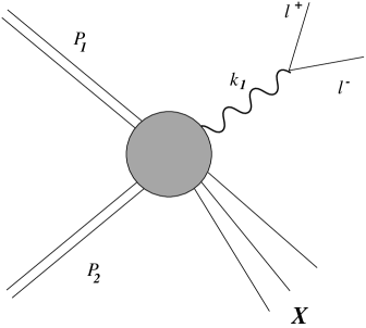
Figure 1: The Drell-Yan process

There are at least two reasons to justify a detailed NLO study of the Drell Yan (DY) process, Fig. 1, both in the case of the longitudinal and of the transverse asymmetries. The first one is that the final state is particularly “clean”, due to the presence of a lepton pair. This means that the photon fragmentation contribution does not affect the momentum distribution of the final state. In particular, the scale dependence associated to a fragmenting photon is absent.

The second reason is that transverse asymmetries are sensitive to gluon distributions only through radiative corrections. In previous works, the complete (real plus virtual) NLO corrections to the non singlet DY cross section with longitudinally polarized initial states have been presented (for the nonzero $p_{T}\equiv q_{T}$ distributions). In this work we make the first step toward extending these calculations to the case of transversely polarized incoming states.

Although much of the experimental data are usually collected at small $p_{T}$, the study of the distributions at large $p_{T}$ remains, nevertheless, a challenging and complex problem.

As a results of these studies, we are able to perform nontrivial perturbative checks of factorization in QCD and we developed more complete strategies for the investigation of spin dependent cross sections. Most of the techniques that we consider in this and in former related [3] work are, in fact, applicable to the easier case of polarized $e^{+}e^{-}$ collisions.

Our analysis is organized as follows. After a discussion of the main features of the various cross sections in the the study of the Drell Yan process, we analyze the properties of the cross section $d\sigma/d^{4}q\,\,d\Omega$.

We separate the contributions to this cross section into “diagonal” and “non-diagonal” terms, and then we give very compact results for the virtual corrections to the “diagonal” terms. The term “diagonal” refers to those contributions obtained by contracting the hadronic tensor (at parton level) with the $g^{\mu\nu}$ part of the leptonic tensor, while the “non-diagonal” part contains the momenta of the lepton pair (here denoted as $v_{1}^{\mu}v_{2}^{\nu}$). We show that these “diagonal” virtual corrections factorize. The result is presented in a remarkably simple form. The reason for performing this separation comes from the structure of the factorized cross section in terms of parton distributions as given originally by Ralston and Soper in the parton model [7]. We will come back to this point briefly in one of the following sections.

Then we move to a detailed discussion of the real emission contributions and show that in our cross section the integration over 3 of the five final-state partons is sufficient to cancel the singularities of the virtual corrections. We will not give here simplified results for the real emissions, which will be presented elsewhere, but we set up the stage for a complete analysis of the real emissions to NLO. Some relevant technical aspects of the calculation have been included in various appendices. A very efficient method to perform the renormalization of all the diagrams -which is of simple symbolic implementation- is illustrated in some detail, since it is of general applicability. In a concluding section we summarize our analysis and elaborate on future developments and unsolved issues of the theory.

Figure 2: Leading order contribution to the Drell-Yan process

2 Zero $p_{T}$ distributions. General Features

Let $H_{1}$ and $H_{2}$ be two polarized hadron that collide thereby producing a heavy photon and some hadronic remnants (X)

$$H_{1}+H_{2}\to\gamma^{*}+X.$$ (1)

At parton level the process goes through the elementary scattering

$$a+b\to\gamma^{*}\to l^{+}+l^{-},$$ (2)

and the leading channel is the annihilation channel. The process is purely electromagnetic at the lowest order. In fact, Fig. 2 is the leading order contribution to the DY process. At this order, the lepton pair is produced with a total zero $q_{T}$, i.e. back-to-back.

If we include radiative corrections -with an additional parton in the final state beside the photon- then the lepton pair gets a nonzero $q_{T}$. Two cross sections are studied in general: $\sigma(Q^{2})$ and $d\sigma/dy\,dx_{F}$, with y being the rapidity of the photon and $x_{F}$ is its “Feynman’s x”. Both cross sections are sufficiently inclusive and well defined in perturbation theory so that an analytic calculation is possible.

The NLO corrections to the $\sigma(Q^{2})$ cross section are quite straightforward to obtain. At this order, for instance, the real emissions involve only 2 partons in the final state, while the virtual require the 1-loop renormalized $q\,\,\bar{q}\,\,\gamma^{*}$ vertex plus quark self-energy insertions (see Fig. 3).

Figure 3: $\alpha_{s}$ order contributions

In this cross section one of the final state partons is integrated over (the gluon or the quark) and the transverse momentum dependence of the lepton pair is not completely resolved.

A better accuracy is obtained by going to NNLO, i.e. at order $\alpha_{s}^{2}$.

For instance, in the non-singlet sector, all the diagrams $V_{1},...,V_{11}$ (Fig. 7) are needed, plus there are contributions from the so called “G”, “F” and “H” sets (see Figs. 4-6). Basically, the G-set involves real emissions of the form $q\bar{q}\to gg\gamma^{*}$; the set F involves both annihilation ($q\bar{q}\to q\bar{q}\gamma^{*}$) and scattering $(q\bar{q}\to q\bar{q}\gamma^{*})$ diagrams, while the set $H$ involves $qq^{\prime}\to qq^{\prime}\gamma^{*}$ scattering diagrams.

Additionally, one needs to evaluate all the corrections coming from the interference between the 2-loop (polarized) on-shell quark form factor and the lowest order process of Fig 2. The latter are the only two-loop contributions needed for a complete NNLO calculation of the invariant mass distribution.

In a completely anticommuting scheme for $\gamma_{5}$ this can be obtained directly from the literature, and differs from the result of refs. [12] just by an overall helicity factor $(1-h)$. In the t’Hooft-Veltman scheme it is expected that additional helicity-violating terms will appear, since the on-shell form factor is not infrared (IR) safe. However, a redefinition of the polarized splitting function of the form $\Delta P_{qq}=P_{qq}+4C_{F}\epsilon(z-1)+O(\epsilon^{2})$ should be sufficient to eliminate the helicity-violating contributions. However, as we have mentioned before, the invariant mass distribution has to be analyzed both in its diagonal and non-diagonal contributions in order to obtain information on the perturbative corrections to the transverse spin cross section. In fact, as we will discuss below, it is the structure of the parton model result for $\sigma^{TT}$ that forces us to consider a more general approach to the DY process, and renders the calculation far more complex than in the unpolarized or in the longitudinally polarized case.

3 Nonzero $p_{T}$ Distributions

Since there is a lot of information in the transverse momentum distribution of the lepton pair and since, experimentally, one needs to set cuts below a certain $p_{T}$, the study of the transverse momentum distributions turns out to be of considerable interest. Various cross sections are studied for this purpose. One of the most studied cross section is defined as $d\sigma/d^{2}Q_{T}$, or, equivalently as $d\sigma/dt\,\,du$. In the analysis of the virtual corrections we will concentrate on the latter. We remind that the diagonal part of the more general cross section $d\sigma/d^{4}q\,d\Omega$, with $\Omega$ defined to be the solid angle in the rest frame of the photon, is easily extracted from $d\sigma/dt\,\,du$. In their non-diagonal contributions the two cross sections are, of course, different.

The distribution cross section $d\sigma/dt\,du$ starts at order $\alpha_{s}$ and the two diagrams $L_{1}$ and $L_{2}$ denote its two Born level contributions in the non-singlet sector, and proceeds to NLO (or $O(\alpha_{s}^{2})$) through the radiative corrections of Figs. 4–7.

The virtual and the real corrections to this cross sections are the same corrections that appear in the NNLO analysis of $\sigma(Q^{2})$, the invariant mass distribution.

The extension of $d\sigma/dt\,du$ to the small $q_{T}$ region can be performed by a resummation [20] in impact parameter. At large $q_{T}$, instead, the cross section is perfectly well defined.

If we use Dimensional Regularization (DR) (with $n=4-2\epsilon$) to calculate both the real and the virtual corrections to this cross section, then the overlapping soft and collinear regions of integration will produce double poles $1/\epsilon^{2}$ and the collinear regions single $1/\epsilon$ poles. The study of this cross sections in the non-singlet sector shows that “factorization” takes place both for the unpolarized [4] and for the longitudinally polarized case [3]. By “factorization” here we mean that the double poles will cancel between the real and the virtual contributions, while the left over collinear singularities “factorize”, i.e. can be absorbed into universal parton distributions, which are process independent. The usual factorization picture involves also a collinear expansion of the momenta of the hard scatterings around a light-cone direction, fixed by the large momenta of the two colliding hadrons, and arrested at a certain order. Parton distributions of various twist, in this picture, are defined as matrix elements of nonlocal operators at light-like separations. Natural ways to incorporate into this picture contributions of higher twist and proofs of factorization [19] have also been formulated.

An important part of the analysis is the proof of the gauge invariance of the factorization formula up to a certain twist. The operatorial expansion of [9] shares the same features of ref. [19], although the analysis is performed directly on the light-cone, rather than in momentum space [19].

In both formulations, the violations to the scaling behaviour of the twist 2 (and of any twist) structure functions are purely logarithmic, at any order in perturbation theory and all the hard scatterings -for distributions of any twist- are calculated in the collinear approximation.

These approaches, which are manifestly gauge invariant, do not isolate any transverse (explicit) $q_{T}$ in the dominant cut-diagram describing the factorization formula. Isolation of a fixed $q_{T}$ in the parton distributions brings the operatorial expressions that describe these distributions away from the light cone.

In the following, we will assume that the leading cut-diagram describing the Drell Yan process at nonzero $p_{T}$ contains a hard scattering of the form $L_{1}$ or $L_{2}$. Therefore, in the leading twist approximation, the $q\bar{q}$ partons undergo hard scattering with purely collinear light-like momenta. The $q_{T}$ of the photon, therefore, is not “intrinsic”, as discussed in [7, 11], but it is due to the real (lowest order) emission of a gluon. The scaling ($\ln q_{T}$) violations to this basic picture are generated by the additional radiative corrections of Figs. 4-7.

4 $\sigma(Q^{2})$ versus $d\sigma/dt\,du$

In order to obtain $\sigma(Q^{2})$ from $d\sigma/dt\,\,du$, then we need to integrate the latter cross section in $t$ and $u$. By doing so, we will generate additional singularities (up to $1/\epsilon^{4}$) after integration, since the transverse momentum distribution contains matrix elements of the form $1/t$, $1/u$, $1/u\,\,t$ etc, which will be responsible for higher order poles in $\epsilon$. These higher order singularities, according to factorization, will cancel in the final sum of real and virtual, after adding the contributions coming from the two-loop on-shell quark form factor.

Therefore, the $O(\epsilon^{0})$ radiative corrections to the cross section $d\sigma/dt\,\,du$ gives, after $t-u$ integration, only the $bulk$ of the total NNLO corrections to the invariant mass distribution. These corrections, in the longitudinally polarized case, have been calculated [6].

5 $d\sigma/d^{4}q\,\,d\Omega$ and transverse spin at nonzero $P_{T}$

In their pioneering paper on the polarized Drell Yan process, Ralston and Soper [7] introduced the notion of transverse parton distributions. It is by now well established that $h_{1}(x)$ is a leading twist (or twist 2) distributions which can be measured in p-p collisions using transversely polarized beams.

As we are going to see, in order to have a non vanishing projection on the transverse spin distribution of the hadronic tensor, the parton model prediction requires that the lepton pair should not be completely integrated out. The result is common to all the approaches [7, 9, 11] followed so far in the analysis of the parton distributions in polarized collisions.

Here we briefly overview these results in order to make our treatment self contained.

The factorized (parton model) picture of the collision emerges in an infinite momentum frame, with a large boost parameter (formally $P\to\infty$).

In this limit the two colliding hadrons have large “plus” or “minus” components and fields are effectively quantized at equal light-cone time $x^{+}$. The degrees of freedom of a fermion are halved, with the negative $\psi_{-}=1/2\gamma^{-}\gamma^{+}$ (bad or dependent) light-cone projections of the Dirac fermions functions of the positive $\psi_{+}=1/2\gamma^{+}\gamma^{-}$ (good or independent) ones [9, 10], and of the transverse components of the gauge field. The plus components can be labeled by helicity eigenvalues $\psi_{+}^{\pm 1/2}$ and chirality eigenvalues of the same sign. The negative projections are basically interpreted as quark-gluon composites. The requirement that the helicity of the composite be $\pm 1/2$ forces the composite to be of the form $\psi_{-}^{1/2}\sim\psi_{+}^{-1/2}A^{+1}$ and $\psi_{-}^{-1/2}\sim\psi_{+}^{+1/2}A^{-1}$. The chirality of the bad quantum components have flipped sign compared to the helicities. While the distributions $f_{1}(x)$ and $g_{1}(x)$ have a natural interpretation (i.e. are diagonal) in the chirality/helicity basis, the distribution $h_{1}(x)$ does not. Since a fermion of fixed transverse spin is in an eigenstate of the Pauli-Lubanski operator, it is convenient to expand the components of the fermion in a basis of eigenstates of such operator (transversity basis), which are expressible as linear combinations of the helicities. $h_{1}(x)$ then measures the number of quarks polarized in the transverse direction minus the number of those polarized in the opposite direction in a transverse polarized hadron (at a fixed light-cone momentum fraction x).

One starts by defining the hadronic tensor

$$W^{\mu\nu}=\int{d^{4}x\over 2(\pi)^{4}}e^{iq\cdot x}\langle P_{A}S_{A};P_{B}S_{B}|\left[J^{\mu}(0),J^{\nu}(x)\right]|P_{A}S_{A};P_{B}S_{B}\rangle,$$ (3)

with $P_{A}$ and $P_{B}$ being the momenta of the colliding hadrons and $S_{A}$ and $S_{B}$ their covariant spins. In a collinear basis

$$P_{A}=P_{A}^{+}n^{+}+{M^{2}\over 2P_{A}^{+}}n^{-},$$

$$P_{B}=P_{B}^{-}n^{-}+{M^{2}\over 2P_{B}^{-}}n^{+},$$

$$S_{A}={\lambda_{A}P_{A}^{+}\over M}n^{+}-{\lambda_{A}M\over 2P_{A}^{+}}n^{-},$$

$$S_{A}={\lambda_{B}P_{B}^{-}\over M}n^{-}-{\lambda_{B}M\over 2P_{B}^{-}}n^{+},$$ (4)

with spin vectors orthogonal to the hadron momenta.

$P_{A}^{+}$ ands $P_{B}^{-}$ are the two large light-cone components of the incoming hadrons, of equal mass $M$.

Assuming factorization, the quantum numbers of the two hadrons can be decoupled by Fierz transformations, and the interaction described at leading order by a single hard scattering, with a single photon in the unitarity diagram.

The distribution functions that emerge -at leading order- from this factorized picture are correlation functions of non-local operators in configuration space. They are the quark-quark and the quark-antiquark correlators.

Their expression simplifies in the axial gauge, in which the gauge link is removed by the gauge condition. For instance, the quark-quark correlator takes the form

$$\left(\Phi_{a/A}\right)_{\alpha\beta}(P,S,k)=\int{d^{4}z\over(2\pi)^{4}}e^{ik\cdot z}\langle P,S|\overline{\psi}^{(a)}_{\beta}(0)\psi^{(a)}_{\alpha}(z)|PS\rangle.$$ (5)

We have included the quark flavour index $a$ and an index $A$ for the hadron, as usual. Fields are not time ordered since they can be described by the good light cone components $\psi_{+}$ and $A_{T}$, as discussed in [8].

Using hermicity, parity and time reversal invariance, one can give a general expansion for these correlators in terms of basic amplitudes which are functions of P,S, k and are Dirac algebra valued.

However, the basic matrix elements that appear in leading power factorization are not the correlators themselves, but their integrals over the $k^{-}$ and $k_{T}$ components of momentum.

Specifically, one introduces the Sudakov expansion

$$k=xp^{+}n^{+}+{k^{2}-k_{T}^{2}\over 2x}n^{-}+k_{T}$$ (6)

and may decide to integrate over both $k^{-}$ and $k_{T}$ in (5).

Using the identity

$$\int{d(k\cdot p)d^{2}k_{T}\over(2\pi)^{4}}e^{ik\cdot z}=\int{d\lambda\over 2\pi}\delta^{4}(z-\lambda n)e^{i\lambda x},$$ (7)

and projecting over the Dirac basis of the 16 independent $\gamma$ matrices, one obtains the general expansion of the correlator

$$\int\phi={\bf 1}{1\over 4}\int Tr\left[\Phi\right]-i\gamma_{5}\int Tr\left[i\gamma_{5}\Phi\right]+\gamma_{\mu}{1\over 4}\int Tr\left[\gamma^{\mu}\Phi\right]$$

$$\hskip 56.9055pt+\gamma_{5}\gamma_{\mu}{1\over 4}Tr\left[\gamma_{\mu}\gamma_{5}\Phi\right]+i\gamma_{5}\sigma^{\mu\nu}\int Tr\left[i\sigma^{\mu\nu}\gamma_{5}\Phi\right],$$ (8)

where the sign of integration $\int$ is a shorthand notation for the $k^{-},k_{T}$ integration in $k$

$$\int Tr\left[\Gamma\Phi\right] \equiv {1\over 2}\int d(k\cdot p)d^{2}k_{T}Tr\left[\Gamma\Phi(k)\right]$$ (9)

$$= \int{d\lambda\over{4\pi}}e^{i\lambda x}\langle P,S|\overline{\psi}(0)\Gamma\psi(\lambda n)|PS\rangle.$$

Therefore, after integration, the correlators are sampled on light-cone rays.

The transverse spin distribution $h_{1}(x)$ appears in the projector of the quark-quark correlator over $i\sigma^{\mu\nu}\gamma_{5}$

$$\int{d\lambda\over 4\pi}e^{i\lambda x}\langle PS|\overline{\psi}(0)i\sigma^{\mu\nu}\gamma_{5}\psi(\lambda n)|PS\rangle = (S_{T}^{\mu}p^{\nu}-S_{T}^{\nu}p^{\mu})h_{1}(x)$$ (10)

$$+M\lambda(p^{\mu}n^{\nu}-p^{\nu}n^{\mu})h_{L}(x)+M^{2}(S_{T}n^{\nu}-S_{T}^{\nu}n^{\mu})h_{3}(x).$$

Using Jaffe’s definition of twist [10] $t=2+$number of $M$, one finds that $h_{1}(x)$ is twist$-2$, $h_{L}(x)$ is twist$-3$ ands $h_{3}(x)$ is twist$-4$.

The leading twist expansion of the quark-quark correlator then is of the form

$$\int{d\lambda\over 2\pi}e^{i\lambda x}\langle PS|\overline{\psi}(0)\psi(\lambda n)|PS\rangle={1\over 2}\left(\not{p}f_{1}(x)+\lambda\gamma_{5}\not{p}g_{1}(x)+\gamma_{5}\not{S_{T}}\not{p}h_{1}(x)\right).$$ (11)

In their parton model analysis the authors of [9] obtain expressions for the hadron tensor $W^{\mu\nu}$ in terms of parton distributions which are peaked at $q_{T}=0$, (eqs (67), (68) and (69) of [9]).

A more general approach has been discussed in [11]. There, the authors, following Ralston and Soper, assume a factorization with an intrinsic $q_{T}$ for the total momentum of the partons entering hard scattering. The factorized expression for the hadronic tensor is assumed of the form [7, 11]

$$W^{\mu\nu} = {1\over 2}\sum_{ab}\delta_{b\bar{a}}e_{a}^{2}\int d^{4}k_{a}d^{4}k_{b}\delta^{4}(k_{a}+k_{b}-q)$$ (12)

$$\,\,\,\,\,\,\,\,\times Tr[\Phi_{a/A}(P_{A}S_{A},k_{a})\gamma^{\mu}\overline{\Phi}_{b/B}(P_{B},S_{B},k_{b})\gamma^{\mu}].$$

Notice that this primordial $q_{T}$ is not induced by radiative corrections. In this last approach, by setting $q_{=}0$ (or $q_{T}=0$) one is yet unable to recover the results of Jaffe and Ji, since the integrals over the parton momenta $k_{A}$ and $k_{B}$ in the hard scattering are still coupled. They can be uncoupled only if one starts with a general $q_{T}$ in the factorization formula Eq. (12), and integrates over $q_{T}$. Therefore, the approaches of [11, 9] compare at the level of the integrated cross section $d\sigma/dq^{+}dq^{-}d\Omega$, an expression derived originally in [7]. The authors of [11] also claim to be in disagreement with the expression quoted in [9] for the $A_{LT}$ or longitudinal-transverse asymmetry.

The parton level results for the $q_{T}$-integrated cross sections, however, in both approaches, agree, and are also in agreement with the result given by Ralston and Soper, that we simply quote

$${d\sigma\over dq^{+}dq^{-}d\Omega} = {\alpha^{2}\over 4Q^{2}}{1\over 3}\sum e_{Q}^{2}f_{1}(x_{A})f_{1}(x_{B})$$ (13)

$$\times (1-\cos^{2}\theta)(1-\lambda_{A}\lambda_{B}g_{1}(x_{A})g_{1}(x_{B}))$$

$$+\sin^{2}\theta\cos(2\phi-\phi_{A}-\phi_{B})|S_{A}^{T}||S_{B}^{T}|h_{1}(x_{A})h_{1}(x_{B}).$$

The angles $\theta$ and $\phi$ in Eq. (13) refer to the leptons and are measured respect to the Collins-Soper (see below) frame, while $\phi_{A}$ and $\phi_{B}$ are the azimuthal angles of the two transverse spins 4-vectors in the same frame.

It clearly shows that an integration over the azimuthal angle of the lepton pair makes the projection over $h_{1}(x)$ vanish.

6 Parton Level Analysis

Since the structure of the final state in the analysis of the transverse spin cannot be neglected, it is convenient to set up some diagrammatic notations and divide all the calculations into two subsets. Diagrammatically, this is easily understood in terms of cut graphs. For instance, the contraction of the hadronic tensor with the diagonal part (i.e., with $g_{\mu\nu}$) of the leptonic tensor

$$L_{\mu\nu}\sim v_{1\mu}v_{2\nu}+v_{2\mu}v_{1\nu}-g_{\mu\nu}v_{1}\cdot v_{2}$$ (14)

is described in terms of cut diagrams of cross sections for the process $q\bar{q}\to\gamma^{*}$.

The non diagonal part, instead, is schematically described by cut diagrams of cross sections for the process $q\bar{q}\to l^{+}l^{-}$.

In the next sections we will analyze the NLO structure of the non-diagonal non-singlet virtual corrections for the $p_{T}$ distributions.

Notice that if we integrate completely over the final leptons and use the gauge invariance of the partonic matrix elements, then only the diagonal projection survives.

In our calculation we use Dimensional Regularization (DR) all the way. The chiral projectors are regulated according to the t’Hooft-Veltman prescription (HV) [15].

There are clearly many advantages in being able to use this regularization, given the complexity of the calculations. However this is not generally possible in most of cases, except for specifically defined cross sections. As we have just mentioned, the cross section has to be sufficiently inclusive in order to be able to cancel the infrared divergences order by order in perturbation theory. At the same time, in the case of transverse spin, we need to leave in part the lepton pair in the final state unintegrated. As we are going to show in the next sections, one possible choice is given by the cross section $d\sigma/d^{4}q\,\,d\Omega$, with $\Omega$ evaluated in the rest frame of the photon, which we are going to investigate.

7 About the treatment of $\gamma_{5}$

Here are some remarks concerning the extension used for $\gamma_{5}$ in n dimensions. In the t’Hooft-Veltman prescription for $\gamma_{5}$ for $n=4-2\epsilon$ dimensions, the Dirac algebra is split into a 4 and into an $n-4$ subspace.

The metric space is also split in a similar way

$$g^{\mu\nu}=\widehat{\widehat{g}}_{\mu\nu}+\widehat{g}_{\mu\nu},$$ (15)

and the Dirac algebra written as a direct sum

$$\gamma_{\mu}=\widehat{\widehat{\gamma}}_{\mu}+\widehat{\gamma}_{\mu}.$$ (16)

The anticommutation relations for the $\gamma$ matrices are

$$\left[\widehat{\widehat{\gamma}}_{\mu},\widehat{\widehat{\gamma}}_{\nu}\right]_{+}=2\widehat{\widehat{g}}^{\mu\nu},\hskip 14.22636pt\left[{\widehat{\gamma}}_{\mu},{\widehat{\gamma}}_{\nu}\right]_{+}=2{\widehat{g}}^{\mu\nu},\hskip 14.22636pt\left[{\widehat{\gamma}}_{\mu},\widehat{{\widehat{\gamma}}}_{\nu}\right]_{+}=0.\\$$

The antisymmetric tensor $\epsilon_{\mu\nu\rho\sigma}$ is 4 dimensional and projects only over the 4 dimensional subspace

$$\epsilon_{\mu\nu\rho\sigma}\widehat{g}_{\sigma\eta}=0,\hskip 42.67912pt\epsilon_{\mu\nu\rho\sigma}\widehat{\gamma}_{\sigma}=0.$$ (17)

$\gamma_{5}$ is defined in n-dimensions as

$$\gamma_{5}={i\over 4!}\epsilon^{\mu\nu\rho\sigma}\gamma^{\mu}\gamma^{\nu}\gamma^{\rho}\gamma^{\sigma}.$$ (18)

With this definition, $\gamma_{5}$ anticommutes with the 4-dimensional $\gamma$’s and commutes with the remaining the n-4-dimensional ones.

8 Distributions at nonzero $p_{T}$

We calculate the spin dependence of the cross section using the relation [14]

$$u(p,s)\bar{u}(p,s)={1\over 2}p\hskip-6.0pt/\hskip 6.0pt(1-\lambda\gamma_{5}+\gamma_{5}s\hskip-5.0pt/_{\perp})\ ,$$ (19)

where $s_{\perp}$ represents the transverse components of the spin vector $s^{\mu}$, and $s^{\mu}s_{\mu}=-1$. Clearly, $\lambda$ and $|s_{\perp}|$ are not independent, and in fact satisfy the relation $\lambda^{2}+|s_{\perp}|^{2}=1$.

In our NLO calculation $\alpha_{s}\to\alpha_{s}(\mu^{2})$ is the running coupling constant renormalized at the scale $\mu^{2}$ in the $\overline{MS}$ scheme, satisfying the renormalization group equation

$$\mu^{2}\frac{d\alpha_{s}}{d\mu^{2}}=-\alpha_{s}\left[\beta_{0}\frac{\alpha_{s}}{4\pi}+\beta_{1}\left(\frac{\alpha_{s}}{4\pi}\right)^{2}+O(\alpha_{s}^{3})\right]\ ,$$ (20)

with

$$\beta_{0} = \frac{11N_{C}}{3}-\frac{2N_{F}}{3}$$

$$\beta_{1} = \frac{34N_{C}^{2}}{3}-\frac{10N_{C}N_{F}}{3}-2C_{F}N_{F}\ ,$$ (21)

and with $N_{F}$ the number of active quark flavors.

The lowest order (non-singlet) contributions to the real emissions arise from the two, $q+\bar{q}\to\gamma^{*}+g$, amplitudes $L_{1}$ and $L_{2}$. As mentioned before, they are also the lowest order contributions to the $p_{T}$ distributions in Drell Yan.

We refer to these two diagrams as the direct and the exchange (or crossed) amplitudes, respectively.

The squares of the direct amplitude $L_{1}$ and exchange amplitude $L_{2}$ in Fig. 3 in $n=4-2\epsilon$ dimensions are given by

$$M_{dd}(s_{1},s_{2}) = e_{f}^{2}g^{2}g_{s}^{2}{C_{F}\over N_{c}}{2u\over t}\left[(1-\epsilon)^{2}-h(1+\epsilon)^{2}\phantom{\frac{1}{1}}\right.$$

$$\left.\hskip 28.45274pt-\epsilon^{2}\left(s_{1\perp}\cdot s_{2\perp}+{2s\over tu}(k_{2}\cdot s_{1\perp})(k_{2}\cdot s_{2\perp})\right)\right],$$

$$M_{cc}(s_{1},s_{2}) = e_{f}^{2}g^{2}g_{s}^{2}{C_{F}\over N_{c}}{2t\over u}\left[(1-\epsilon)^{2}-h(1+\epsilon)^{2}\phantom{\frac{1}{1}}\right.$$ (22)

$$\left.\hskip 28.45274pt-\epsilon^{2}\left(s_{1\perp}\cdot s_{2\perp}+{2s\over tu}(k_{2}\cdot s_{1\perp})(k_{2}\cdot s_{2\perp})\right)\right].$$

$e_{f}$ the charge of the quark, and we have set $\lambda_{1}\lambda_{2}=h$. The quantity $C_{F}/N_{c}$ is the color factor, and $\alpha_{s}=g_{s}^{2}/4\pi$ is the QCD strong coupling constant.

The interference term is more complicated and is given by,

$$2M_{dc}(s_{1},s_{2})=$$

$$e_{f}^{2}g^{2}g_{s}^{2}{C_{F}\over N_{C}}{4\over tu}\left[(1-\epsilon)(Q^{2}s-\epsilon tu)-h(1+\epsilon)(Q^{2}s+\epsilon tu)-2h\epsilon tu\right.$$

$$\left.+(s_{1\perp}\cdot s_{2\perp})((Q^{2}s+tu)-(1+\epsilon)(Q^{2}s+\epsilon tu))\right.$$

$$\left.+\left({(k_{2}\cdot s_{1\perp})(k_{2}\cdot s_{2\perp})\over Q^{2}}\right)(2sQ^{2}(1-\epsilon-\epsilon^{2}))\right].$$ (23)

The sum of the two Born amplitudes squared is

$$|M_{B}(s_{1},s_{2})|^{2}=M_{dd}(s_{1},s_{2})+2M_{dc}(s_{1},s_{2})+M_{cc}(s_{1},s_{2})$$

$$=e_{f}^{2}g^{2}g_{s}^{2}{C_{F}\over N_{C}}{2\over tu}\left[(1-h)(1-\epsilon)\left(2Q^{2}s+(1-\epsilon)(t^{2}+u^{2})-2\epsilon tu\right)\right.$$

$$\,+4h\epsilon\left(Q^{2}s+(u+t)^{2}\right)$$

$$\,+(s_{1\perp}\cdot s_{2\perp})\left(2tu-2\epsilon(s+u)(s+t))-\epsilon^{2}(t+u)^{2}\right)$$

$$\left.+\left({(k_{2}\cdot s_{1\perp})(k_{2}\cdot s_{2\perp})\over tu}\right)2s(2tu(1-\epsilon)-\epsilon^{2}(t+u)^{2})\right].$$ (24)

The distribution cross section is defined by

$$s{d\hat{\sigma}_{B}\over dt}=e_{f}^{2}K_{2}{\alpha_{s}\over s}\left[T_{1}(Q^{2},u,t,h)+T_{2}(Q^{2},u,t,s_{\perp 1},s_{\perp 2})\right].$$ (25)

$K_{2}$ is defined by

$$K_{2}=\pi\alpha{C_{F}\over N_{C}}{1\over\Gamma(1-\epsilon)}\left({4\pi\mu^{2}\over Q^{2}}\right)^{\epsilon}\left({sQ^{2}\over tu}\right)^{\epsilon},$$ (26)

where we have rescaled, $\alpha_{s}\to\alpha_{s}(\mu^{2})^{\epsilon}$, so that it remains dimensionless in $n=4-2\epsilon$ dimensions. The first component of the cross section is the same as longitudinally polarized cross section

$$T_{1}(Q^{2},u,t,h)=(1-h)T_{B}(Q^{2},u,t)+8h\epsilon\frac{Q^{2}s+(u+t)^{2}}{tu}$$ (27)

where $T_{B}$ is the unpolarized born level matrix element.

$$T_{B}(Q^{2},u,t)=2(1-\epsilon)\left[(1-\epsilon)\left(\frac{u}{t}+\frac{t}{u}\right)+\frac{2Q^{2}(Q^{2}-u-t)}{ut}-2\epsilon\right].$$ (28)

The transverse spin contribution to the cross section is

$$T_{2}(Q^{2},u,t,s_{1\perp},s_{2\perp}) = 2s_{1\perp}\cdot s_{2\perp}\frac{2tu-2\epsilon(s+u)(s+t)-\epsilon^{2}(t+u)^{2}}{tu}$$ (29)

$$+4(k_{1}\cdot{s}_{1\perp})(k_{1}\cdot{s}_{2\perp})\frac{s(2(1-\epsilon)tu-\epsilon^{2}(t+u)^{2})}{t^{2}u^{2}}$$

$$= 2\beta\left(2(1-\epsilon)-\epsilon^{2}\frac{(t+u)^{2}}{tu}\right)-4\epsilon(s_{1\perp}\cdot s_{2\perp})\frac{sQ^{2}}{tu},$$

where

$$\beta=\frac{2(k_{1}\cdot{s}_{1\perp})({k}_{1}\cdot{s}_{2\perp})s}{tu}+{s}_{1\perp}\cdot{s}_{2\perp}.$$ (30)

If $s_{1\perp}=s_{2\perp}=0$, Eq. (25) reduced to the longitudinally polarized cross section cross section of Ref. [3].

In the limit $h=0$

$$\vec{s}_{1\perp}\cdot\vec{s}_{2\perp}=-s_{1\perp}\cdot s_{2\perp}=\cos\Delta\theta$$ (31)

and

$$\frac{2(k_{1}\cdot{s}_{1\perp})({k}_{1}\cdot{s}_{2\perp})s}{tu}+{s}_{1\perp}\cdot{s}_{2\perp} = \frac{2(\vec{k}_{1}\cdot\vec{s}_{1\perp})(\vec{k}_{1}\cdot\vec{s}_{2\perp})s}{tu}-\vec{s}_{1\perp}\cdot\vec{s}_{2\perp}$$ (32)

$$= \frac{2k_{\perp}^{2}s}{tu}\cos\theta_{1}\cos(\theta_{1}+\Delta\theta)-\cos\Delta\theta$$

$$= \cos(2\theta_{1}+\Delta\theta).$$

Here, $k_{\perp}^{2}=(tu)/s$ and $\theta_{1}$ is an angle between $\vec{k}_{\perp}$ and $\vec{s}_{1\perp}$.

Away from 4 dimensions $T_{1}$ clearly contains helicity violating contributions, due to the prescription chosen for $\gamma_{5}$.

9 The Structure of the Non Singlet

The radiative corrections to the non singlet come from the interference between the two diagrams $L_{1}$ and $L_{2}$ and the diagrams denoted $V_{1},....V_{11}$

$$d{\hat{\sigma}}^{virtual}\sim 2Re\left((L_{1}+L_{2})\sum_{i=1}^{11}V_{i}^{*}\right),$$ (33)

The other real $\bar{q}_{f}q_{f}$ diagrams are

$$d{\hat{\sigma}}^{real}_{\bar{q}_{f}q_{f}}\sim|\sum_{i=1}^{8}F_{i}|^{2}+|\sum_{i=1}^{8}G_{i}|^{2},$$ (34)

where the amplitudes $F_{i}$ are shown in Fig. 4 and the amplitudes $G_{i}$ are shown in Fig. 5 with $f=f^{\prime}$. The absolute square of the $F_{i}$ amplitudes can be written as:

$$|\sum_{i=1}^{8}F_{i}|^{2}=$$ (35)

$$|F_{1}+F_{2}|^{2}+|F_{3}+F_{4}|^{2}+2Re\left(\sum_{i=1}^{4}F_{i}\sum_{i=5}^{8}F^{*}_{i}\right)+|\sum_{i=5}^{8}F_{i}|^{2},$$

having used

$$Re\left((F_{1}+F_{2})(F_{3}+F_{4})^{*}\right)=0.$$ (36)

Therefore, the diagonal real $\bar{q}_{f}q_{f}$ contributions are

$$d{\hat{\sigma}}^{real}_{\bar{q}_{f}q_{f}}=d{\hat{\sigma}}_{1}+d{\hat{\sigma}}_{2}+d{\hat{\sigma}}_{3}+d{\hat{\sigma}}_{F},$$ (37)

where

$$d{\hat{\sigma}}_{1} \sim |F_{1}+F_{2}|^{2}+|\sum_{i=1}^{8}G_{i}|^{2},$$ (38)

$$d{\hat{\sigma}}_{2} \sim |F_{3}+F_{4}|^{2},$$ (39)

$$d{\hat{\sigma}}_{3} \sim 2Re\left(\sum_{i=1}^{4}F_{i}\sum_{i=5}^{8}F^{*}_{i}\right),$$ (40)

$$d{\hat{\sigma}}_{F} \sim |\sum_{i=5}^{8}F_{i}|^{2}.$$ (41)

The real diagonal $q_{f}\,q_{f}$ diagrams are

$$d{\hat{\sigma}}^{real}_{q_{f}q_{f}}\sim|\sum_{i=1}^{4}H_{i}-\sum_{i=4}^{8}H_{i}|^{2},$$ (42)

where the amplitudes $H_{i}$ are shown in Fig. 6 and the relative minus sign between the direct and exchange diagrams is due to Fermi statistics since $f=f^{\prime}$. The absolute square of the $H_{i}$ amplitudes can be written as follows:

$$|\sum_{i=1}^{4}H_{i}-\sum_{i=4}^{8}H_{i}|^{2}=$$ (43)

$$|\sum_{i=1}^{4}H_{i}|^{2}+|\sum_{i=4}^{8}H_{i}|^{2}-2Re\left(\sum_{i=1}^{4}H_{i}\sum_{i=4}^{8}H_{i}^{*}\right).$$

Thus the diagonal real $q_{f}q_{f}$ contributions are,

$$d{\hat{\sigma}}^{real}_{q_{f}q_{f}}=d{\hat{\sigma}}_{H}+d{\hat{\sigma}}_{4},$$ (44)

where

$$d{\hat{\sigma}}_{H} \sim |\sum_{i=1}^{4}H_{i}|^{2}+|\sum_{i=4}^{8}H_{i}|^{2},$$ (45)

$$d{\hat{\sigma}}_{4} \sim -2Re\left(\sum_{i=1}^{4}H_{i}\sum_{i=4}^{8}H_{i}^{*}\right).$$ (46)

The diagonal ($f=f^{\prime}$) real part of the non-singlet cross section is given by subtracting (42) from (37) as follows:

$$d{\hat{\sigma}}^{real}_{NS}=d{\hat{\sigma}}_{1}+d{\hat{\sigma}}_{2}+d{\hat{\sigma}}_{3}-d{\hat{\sigma}}_{4},$$ (47)

where we have used the fact that $d{\hat{\sigma}}_{F}=d{\hat{\sigma}}_{H}$ which arises due to

$$\int_{PS_{3}}|\sum_{i=5}^{8}F_{i}|^{2}=\hbox{${1\over 2}$}\int_{PS_{3}}|\sum_{i=1}^{4}H_{i}|^{2}+\hbox{${1\over 2}$}\int_{PS_{3}}|\sum_{i=4}^{8}H_{i}|^{2}.$$ (48)

When integrating over the two identical particles $k_{3}$ and $k_{4}$ over the phase space $PS_{3}$ in (63) an extra statistical factor of $1/2$ must be inserted so as not to double count. Thus, the diagonal ($f=f^{\prime}$) part of the complete non-singlet cross section is given by

$$d{\hat{\sigma}}_{NS}=d{\tilde{\sigma}}_{1}+d{\hat{\sigma}}_{2}+d{\hat{\sigma}}_{3}-d{\hat{\sigma}}_{4},$$ (49)

where

$$d{\tilde{\sigma}}_{1}=d{\hat{\sigma}}^{fact}_{1}+d{\hat{\sigma}}^{virtual},$$ (50)

and where $d{\hat{\sigma}}^{fact}_{1}$ is the “factorized” cross section given by

$$d{\hat{\sigma}}^{fact}_{1}=d{\hat{\sigma}}_{1}+d{\hat{\sigma}}^{counter}_{1}.$$ (51)

It is necessary to remove the collinear singularities from the initial state by subtracting the cross section $d{\hat{\sigma}}^{counter}_{1}$ to $d{\hat{\sigma}}_{1}$.

The off-diagonal real $\bar{q}_{f}q_{f^{\prime}}$ diagrams are

$$d{\hat{\sigma}}^{real}_{\bar{q}_{f}q_{f^{\prime}}}\sim|\sum_{i=1}^{4}F_{i}|^{2},$$ (52)

where the amplitudes $F_{i}$ are shown in Fig. 4 and where $f\neq f^{\prime}$. Similarly, the off-diagonal real $q_{f}q_{f^{\prime}}$ diagrams are

$$d{\hat{\sigma}}^{real}_{q_{f}q_{f^{\prime}}}\sim|\sum_{i=1}^{4}H_{i}|^{2},$$ (53)

where the amplitudes $H_{i}$ are shown in Fig. 6. In this case,

$$|\sum_{i=1}^{4}F_{i}|^{2}=|\sum_{i=1}^{4}H_{i}|^{2},$$ (54)

and these two contributions cancel when forming the non-singlet cross section.

The total contribution to the transversely polarized cross section can then be written in the form

$$d\sigma=d\sigma_{NS}+2\left(d\sigma_{H}+d\sigma_{4}\right)_{ff}+\left(d\sigma^{real}_{q_{f}q_{f^{\prime}}}+d\sigma^{real}_{q_{f}\bar{q}_{f^{\prime}}}\right),$$ (55)

where the suffix $ff$ refers the diagonal (in flavour) contribution and the remaining term in bracket are the off diagonal scattering diagrams in the F and H sets.

10 Off-shell renormalization and tensor reductions

Although in the non-singlet sector we do not encounter any anomalous diagram, the regularization scheme still suffers from unphysical features, such as helicity violation, which are absent in other schemes. We should also mention that in the case of the 2-to-2 contributions, all the dependence on the hat-momenta of the the hard scattering can be eliminated. This is equivalent to ask that the momenta which are not integrated -and also the spin 4-vectors- have only 4 dimensional components.

The calculation of the radiative corrections to the vertices is often performed by using various tricks in order to simplify the loop momenta, such as the Feynman parameterization combined with symmetric integration. An alternative way to proceed is to use the Passarino-Veltman (PV) [18] recursion procedure in order to relate the tensor integrals which appear in the calculation to the corresponding scalar ones. The PV method introduces scaless integrals which have to be handled with particular care. In an appendix we illustrate in a simple way how to obtain the renormalized expression of all the coefficients of the expansion of tensor integrals to scalar form. The approach [6] is easy to implement in symbolic manipulations. We start from the expression of any tensor integral and apply the Passarino Veltman (PV) reduction procedure to determine the coefficients of the expansion. Only the renormalization of the scalar self energy diagram $B_{0}(Q^{2})$ (and of its $Q^{2}\to 0$ limit) is needed. We use dimensional regularization with a single parameter $\epsilon$ to regulate both UV and IR singularities. Notice that scaless integrals such as $B_{0}(0)$, so generated, are intrinsically ambiguous. While it is possible to set such terms to zero by definition (on-shell), off-shell renormalization of $B(Q^{2})$ leaves us with a $1/\epsilon$ pole contribution in $B_{0}(0)$ after that the $Q^{2}\to 0$ limit is performed. We isolate and remove the UV singularity (by setting $n=4-2\epsilon$), we then switch $\epsilon\to-\epsilon$ to regulate the remaining IR divergences. Finally, we send $Q^{2}\to 0$. This leaves us with a $1/\epsilon$ pole for $B_{0}(0)$, of IR origin. Details of the method can be found in the appendix.

11 NLO Diagonal Virtual Corrections

In this section we present results for the diagonal corrections to the NLO non-singlet cross section and show their factorization. Although the evaluation of these diagrams is a formidable task, the result can be condensed in a remarkably simple form. We get

$$\!\!\!\!\!\!\!\!\!\frac{sd\sigma^{\rm virtual}}{dtdu}=e^{2}_{f}K_{2}\frac{\alpha_{s}}{s}\delta(s+t+u-Q^{2})\left\{\left(T_{1}+T_{2}\right)\left[1-\frac{\alpha}{2\pi}\frac{\Gamma(1-\epsilon)}{\Gamma(1-2\epsilon)}\left(\frac{4\pi\mu^{2}}{Q^{2}}\right)^{\epsilon}\right.\right.$$

$$\left.\ \times\left(\frac{2C_{F}+N_{C}}{\epsilon^{2}}+\frac{1}{\epsilon}\left(3C_{F}-2C_{F}\ln\frac{s}{Q^{2}}+\frac{11}{6}N_{C}+N_{C}\ln\frac{sQ^{2}}{ut}-\frac{1}{3}N_{F}\right)\right)\right]$$

$$\left.+\frac{\alpha}{2\pi}\left[(1+h)R_{1}+R_{2}\right]\right\},$$ (56)

where

$$\!\!\!\!\!\!\!\!\!R_{1}=\pi^{2}(4C_{F}+N_{C})\frac{2Q^{2}s+t^{2}+u^{2}}{3tu}-2(2C_{F}-N_{C})\frac{Q^{2}(t^{2}+u^{2})}{tu(t+u)}$$

$$-2C_{F}\left(\frac{8(2Q^{2}s+t^{2}+u^{2})}{tu}-\frac{Q^{4}s(t+u)}{tu(s+t)(s+u)}-\frac{t^{2}+u^{2}}{(s+t)(s+u)}\right)$$

$$+\left[\left\{(2C_{F}-N_{C})Li_{2}\left(-\frac{t+u}{s}\right)\frac{2Q^{2}s+t^{2}+u^{2}+2s^{2}}{tu}\right.\right.$$

$$-\left(2Li_{2}\left(\frac{t}{t-Q^{2}}\right)+\ln^{2}\left(\frac{t-Q^{2}}{t}\right)\right)\left(N_{C}\frac{2s+t}{u}+2C_{F}\frac{s^{2}+(s+u)^{2}}{tu}\right)$$

$$+(2C_{F}-N_{C})\left(2\ln\left(\frac{s}{Q^{2}}\right)\frac{Q^{4}-(t+u)^{2}}{(t+u)^{2}}+\ln^{2}\left(\frac{s}{Q^{2}}\right)\frac{s^{2}}{tu}\right.$$

$$\left.-\left(2\ln\left(\frac{|t|}{Q^{2}}\right)\ln\left(\frac{s}{Q^{2}}\right)-\ln^{2}\left(\frac{|t|}{Q^{2}}\right)\right)\frac{s^{2}+(s+u)^{2}}{tu}\right)$$

$$+2\ln\left(\frac{|t|}{Q^{2}}\right)\left(C_{F}\frac{4Q^{2}s-2st+tu}{(s+u)^{2}}+N_{C}\frac{t}{s+u}\right)$$

$$\left.\left.-N_{C}\ln\left(\frac{|t|}{Q^{2}}\right)\ln\left(\frac{|u|}{Q^{2}}\right)\frac{2Q^{2}s+t^{2}+u^{2}}{tu}\right\}+\{t\leftrightarrow u\}\right],$$ (57)

describe the NLO dependence on the longitudinal components of spin. The transverse spin contributions are condensed into the expression

$$\!\!\!\!\!\!\!\!\!R_{2}=(s_{1\perp}\cdot s_{2\perp})\left[\frac{11}{3}N_{C}\frac{Q^{2}s}{tu}+2(2C_{F}-N_{C})\left(\ln\left(\frac{|t|}{Q^{2}}\right)\frac{2s}{s+u}+\ln\left(\frac{|u|}{Q^{2}}\right)\frac{2s}{s+t}\right)\right]$$

$$+\beta\left[(4C_{F}+N_{C})\frac{\pi^{2}}{3}-2C_{F}\left(9+\frac{2s}{t+u}\right)-N_{C}\left(\frac{11}{3}+\frac{(t+u)^{2}}{tu}\right)\right.$$

$$+\left.\left\{2(2C_{F}-N_{C})Li_{2}\left(-\frac{t+u}{s}\right)\frac{s^{2}+u^{2}}{u^{2}}\right.\right.$$

$$-\left(2Li_{2}\left(\frac{t}{t-Q^{2}}\right)+\ln^{2}\left(\frac{t-Q^{2}}{t}\right)\right)\frac{2C_{F}(s^{2}+u^{2})-N_{C}(s^{2}-u^{2})}{u^{2}}$$

$$+(2C_{F}-N_{C})\left(\ln^{2}\left(\frac{s}{Q^{2}}\right)\frac{s^{2}}{u^{2}}-\left(2\ln\left(\frac{|t|}{Q^{2}}\right)\ln\left(\frac{s}{Q^{2}}\right)-\ln^{2}\left(\frac{|t|}{Q^{2}}\right)\right)\frac{s^{2}+u^{2}}{u^{2}}\right)$$

$$+2\ln\left(\frac{|t|}{Q^{2}}\right)\left(3C_{F}-(2C_{F}-N_{C})\left(\frac{2u}{t}+\frac{s+u}{u}+\frac{2u}{s+u}\right)\right)$$

$$\left.\left.-2N_{C}\ln\left(\frac{|t|}{Q^{2}}\right)\ln\left(\frac{|u|}{Q^{2}}\right)\right\}+\{t\leftrightarrow u\}\right].$$ (58)

Notice that in the rest frame of the photon, $\beta=s_{1\perp}\cdot s_{2\perp}$, and the expression above simplifies substantially. From Eq.  (56) it appears obvious that the virtual corrections factorize. In fact the double poles $1/\epsilon^{2}$ correctly multiply the 2-to-2 Born cross section calculated in n dimensions, evaluated with the most general spin dependence in the initial state. If we send any of the transverse spin vectors to zero, then the result coincides with the longitudinally polarized corrections obtained in ref.  [3]. Finally, by sending to zero any of the helicities and any of the 2 spin vectors, one reobtains the result given in ref. [4] in the unpolarized case. Eq. (56) clearly contains (finite) helicity violating contributions which are not canceled by the real emissions in the $\overline{MS}$ scheme. Finite subtractions are needed in order to restore helicity conservation at parton level [3]. A discussion of the longitudinal contributions to the real emissions, which are a subset of the total emissions considered here -and briefly analyzed below- can be found in [3].

12 The qg sector and the Asymmetries

When the incoming quark and the incoming gluon are both transversely polarized, the scattering matrix element is zero.

On the contrary of the longitudinal case (LL scattering), in which the process takes contributions from the non-singlet and from the singlet sector, TT scattering in Drell Yan involves only the quark sector.

This statement can be directly verified to lowest order by an inspection of the Dirac traces, and remains true to all orders in perturbation theory.

To be definite, we introduce 2 (transverse) polarization vectors for the gluon, here denoted as $\epsilon_{1\perp}$ and $\epsilon_{2\perp}$, and choose a collinear base made out of the 2 momenta $p_{1}$ and $k_{2}$, the momenta of the initial state quark and of the final state quark or gluon. $p_{2}$ is the gluon momentum. All these partons are massless: $p_{1}=p_{2}^{2}=k_{2}^{2}=0$.

The two transverse polarizations four-vectors are then defined as

$${\epsilon_{1\perp}}_{\mu}={1\over\sqrt{2(k_{1}\cdot k_{2})(p_{1}\cdot k_{1})(p_{1}\cdot k_{2})}}\left((p_{1}\cdot k_{1}){k_{2}}_{\mu}-(k_{2}\cdot k_{1}){p_{1}}_{\mu}\right)$$

$${\epsilon_{2\perp}}_{\mu}={1\over\sqrt{2(k_{1}\cdot k_{2})(p_{1}\cdot k_{1})(p_{1}\cdot k_{2})}}\epsilon_{\mu\alpha\beta\gamma}p_{1}^{\alpha}k_{2}^{\beta}k_{1}^{\gamma}.$$ (59)

One easily gets

$$\not{\epsilon}_{2\perp}=(\not{p}_{1}\not{k}_{2}\not{p}_{2}-\not{p}_{1}k_{2}\cdot p_{2}+\not{k}_{2}p_{1}\cdot p_{2}-\not{p}_{2}p_{1}\cdot k_{2})\gamma_{5}$$ (60)

which can be easily implemented in symbolic calculations. With these definitions then $\epsilon_{\perp}\cdot k_{1}=\epsilon_{\perp}\cdot p_{2}=\epsilon_{\perp}\cdot k_{2}=0$, which guarantees transversality of the (physical) gluon.

For initial state asymmetries, in order to have a nonvanishing trace, each spinor projector has to contribute with a zero or an even number of gamma matrices. The contribution $\sim\gamma_{5}\not{s}$ is clearly odd and therefore renders the total number of gamma matrices odd (vanishing) in each trace.

A longitudinal quark, however, can scatter from a transverse gluon, since only the $\sim\gamma_{5}\lambda$ part of the fermion projector becomes relevant. These contributions are part of the LL scattering cross section, since we can relate transverse gluon polarizations to the usual gluon helicities by a linear combination $\epsilon^{\pm}=1/\sqrt{2}(\epsilon_{1\perp}\pm i\epsilon_{2\perp})$. The vanishing of $A_{TT}$ in the qg sector indicates that the ratio between $A_{LL}$ and $A_{TT}$ is 1 to lowest order. This simple result shows that Drell Yan plays a key role in the analysis of the transverse spin distributions, since the gluon contributions is absent to all orders.

13 The treatment of the real emissions

In this section we focus our attention on the analysis of the real emissions. The steps that we describe here are necessary in order to proceed with an analytical or a numerical study of the real diagrams.

There are 2 basic modifications to be considered in this case: 1) the presence of a 2-to-4 final phase space integration; 2) the presence of transverse spin in the HV regularization. Some of the features appear already in the longitudinal case, but we prefer to present a comprehensive discussion of all these aspects for future reference.

Let $v_{1}$ and $v_{2}$ denote the momenta of the 2 leptons in the final state. We also set $k_{1}=q$ for notational convenience and introduce the invariants

$$s=(p_{1}+p_{2})^{2},$$

$$s_{12}=(k_{1}+k_{2})^{2},\,\,\,\,s_{23}=(k_{2}+k_{3})^{2},$$

$$t_{1}=(p_{1}-k_{1})^{2},\,\,\,u_{1}=(p_{2}-k_{1})^{2},$$

$$s_{13}=(k_{1}+k_{3})^{2},$$

$$t_{2}=(p_{1}-k_{2})^{2},\,\,\,t_{3}=(p_{1}-k_{3})^{2},$$

$$u_{2}=(p_{2}-k_{2})^{2},\,\,\,\,\,u_{3}=(p_{2}-k_{3})^{2},$$

$${t^{\prime}}_{i}=(p_{1}-v_{i})^{2},\,\,\,\,\,{u^{\prime}}_{i}=(p_{2}-v_{i})^{2}.$$ (61)

Only five of them are independent since

$$s=Q^{2}-(u_{1}+u_{2}+u_{3})=Q^{2}-(t_{1}+t_{2}+t_{3})=s_{12}+s_{23}+s_{13}-2Q^{2},$$

$$s_{12}=s+u_{3}+t_{3},$$

$$s_{23}=s+u_{1}+t_{1}-2Q^{2},$$

$$s_{13}=s+u_{2}+t_{2},$$

$$t_{1}=Q^{2}+{t^{\prime}}_{1}+t^{\prime}_{2},$$

$$u_{1}=Q^{2}+u^{\prime}_{1}+u^{\prime}_{2}.$$ (62)

The integration of the 2-to-4 matrix elements introduces -beside the usual matrix elements of the LL cross section- new matrix elements containing ${t^{\prime}}_{1}$, ${t^{\prime}}_{2}$, ${u^{\prime}}_{1}$ and ${u^{\prime}}_{2}$.

In the separation of the 2-to-4 into 2-to-2 subintegrals, we choose to work in two separate frames 1) the center-of-mass frame of the $k_{2}-k_{3}$ pair; 2) the center-of-mass frame of the photon with axis fixed by the Collins-Soper [21] choice.

To be specific, we start from the 4-particle phase space integral is given by the formula

$$PS_{4}\equiv\!\int\!{d^{n}v_{1}}d^{n}v_{2}\delta_{+}(v_{1}^{2})\delta_{+}(v_{2}^{2}){d^{n}k_{3}}{d^{n}k_{2}}\delta(k_{3}^{2})\delta(k_{2}^{2})\delta^{n}(p_{1}+p_{2}-k_{3}-k_{2}-v_{1}-v_{2}).$$ (63)

We lump together the momenta $k_{3}$ and $k_{2}$ in $k_{23}$ and $v_{1}$ and $v_{2}$ in $q\equiv k_{1}$ as follows

$$PS_{4}=\int d^{n}q\,d^{n}k_{23}\delta^{n}(p_{1}+p_{2}-q-k_{23})\int d^{n}v_{1}\delta_{+}(v_{1}^{2})\delta_{+}((q-v_{1})^{2})$$

$$\times\int d^{n}k_{2}\delta_{+}(k_{2}^{2})\delta_{+}((k_{23}-k_{2})^{2}).$$ (64)

From this expression it is obvious that in the rest frame of the $(2,3)$ pair ($k_{23}$ rest frame) the collinear singularities linked to the two gluons can be easily isolated in Dimensional Regularization.

If hat-momenta are not present, then we easily get

$$PS_{4}=\int d^{n}q\int d^{n}v_{1}\delta_{+}(v_{1}^{2})\delta_{+}((q-v_{1})^{2})\int d^{n}k_{23}\delta^{n}(p_{1}+p_{2}-q-k_{23})$$

$$\hskip 56.9055pt\times\left(k_{23}^{2}\right)^{n/2-2}{\pi^{n/2-2-3/2}\over 2^{n-2}\Gamma[n/2-3/2]}\times I_{12}$$ (65)

where

$$I_{1,2}=\int_{0}^{\pi}d\theta_{1}\sin^{n-3}\theta_{1}\int_{0}^{\pi}d\theta_{2}\sin^{n-4}\theta_{2}$$ (66)

is evaluated in the rest frame of $k_{23}$ and from which the singularities can be exposed.

The final result can be cast in the form

$$PS_{4}=\int d^{n}q\int_{\gamma}d^{n}v_{1}\delta_{+}(v_{1}^{2})\delta_{+}((q-v_{1})^{2})\,s_{23}^{n/2-2}{\pi^{n/2-3/2}\over 2^{n-2}\Gamma[n/2-3/2]}\times I_{1,2},$$ (67)

where we have used the relation $s+t+u=s_{23}+Q^{2}$. The remaining left-over integral has to be evaluated in the photon rest frame, with the Collins-Soper choice of axis. Finally (67) can be expressed in the form

$$PS_{4}=\int d^{n}q\,d\Omega\,\Omega^{n-4}(Q^{2})^{n/2-2}s_{23}^{n/2-2}{\pi^{n/2-3/2}\over 2^{n-2}\Gamma[n/2-3/2]}\times I_{1,2}.$$ (68)

Matrix elements containing ${t^{\prime}}_{1}$ , such as ${t^{\prime}}_{1}/(t_{2}u_{2})$ and similar, can all be exactly evaluated by this procedure, slightly generalized to the tensor case. Matrix elements containing $k_{2}\cdot v_{1}$ (and any denominator) are also easily handled in these two frames. After integration, the result can be conveniently expressed in the Collins-Soper (CS) frame. For this purpose [21] we parameterize the momentum of the photon in a collinear basis defined by the two incoming partons $p_{1}$ and $p_{2}$, and expand $q=x_{1}p_{1}+x_{2}p_{2}+q_{T}$. We introduce two metric projectors $g_{T}$ and $g_{q}$ defined by

$$g_{T}^{\mu\nu}=g^{\mu\nu}-{p_{1}^{\mu}p_{2}^{\nu}\over p_{1}\cdot p_{2}}-{p_{1}^{\nu}p_{2}^{\mu}\over p_{1}\cdot p_{2}}$$

$$g_{q}^{\mu\nu}=g^{\mu\nu}-{q^{\mu}q^{\nu}\over q^{2}}.$$ (69)

These two metrics project in the directions orthogonal to the collinear basis and to q respectively.

An orthonormal set of 4-vectors $(\hat{q},\hat{z},\hat{x},\hat{y})$ is then defined as follows

$$\hat{q}={q^{\mu}\over Q},\,\,\,\,\,\,\,\,\,\,\hat{z}^{\mu}={Z^{\mu}\over\sqrt{-Z^{2}}},\,\,\,\,\,\,\,\,\,\,\hat{x}^{\mu}={X^{\mu}\over\sqrt{-X^{2}}},\,\,\,\,\,\,\,\,\,\,\,\hat{y}^{\mu}={Y^{\mu}\over\sqrt{-Y^{2}}},$$ (70)

where

$$Z^{\mu}=\left({p_{2}\cdot q\over p_{1}\cdot p_{2}}\right)p_{q,1}^{\mu}-\left({p_{1}\cdot q\over p_{1}\cdot p_{2}}\right)p_{q,2}^{\mu},$$

$$X^{\mu}=-\left({p_{2}\cdot Z\over p_{1}\cdot p_{2}}\right)p_{q,1}^{\mu}+\left({p_{1}\cdot Z\over p_{1}\cdot p_{2}}\right)p_{q,2}^{\mu},$$

$$Y^{\mu}={1\over p_{1}\cdot p_{2}}\epsilon^{\mu\nu\rho\sigma}p_{1\nu}p_{2\rho}q_{\sigma},$$

$$p_{q,i}^{\mu}\equiv p_{i}^{\mu}-{p_{i}\cdot q\over q^{2}}q^{\mu}.$$ (71)

The set is orthogonal and spacelike. In the photon rest frame, therefore, it defines a cartesian set of axis. Note that in the collinear frame of the two incoming parton, $Z$ is collinear to $p_{1}$ and $p_{2}$, while $g_{T}$ projects over the transverse (w.r.t. $p_{1}$ and $p_{2}$) plane.

The vector $v_{1}$ can be expanded as

$$v_{1}^{\mu}={q^{\mu}\over 2}+{Q\over 2}\left(\sin\theta\cos\phi\,\hat{x}^{\mu}+\sin\theta\sin\phi\,\hat{y}^{\mu}+\cos\theta\,\hat{z}^{\mu}\right)$$ (72)

and the cross section expressed in a form closer to eq. (13). Finally, one expresses the scalar products $p_{1}\cdot v_{1}$, $q\cdot v_{1}$ or $s_{\perp i}\cdot v_{1}$ in the CS frame.

14 Hat-momenta Integration

As we have mentioned before, the HV prescription introduces matrix elements containing hat-momenta, due to separation of the n-dimensional space into 4 and $n-4$ dimensions. Beside $v_{1}$, the only other hat-momenta expected from the matrix elements are those of $k_{2}$ and $k_{3}$, which are treated in the way discussed below. Other hat-momenta can be eliminated by a convenient choice of axis. This causes, at least in part, a modification of the phase space integral which appear in the unpolarized case.

In the case of unpolarized scattering, the singularities are generated by poles in the matrix elements which have the form $1/t_{3}$, $1/u_{3}$, $1/(t_{3}u_{3})$ and similar ones, in multiple combinations of them. Multiple poles can be reduced to sums of combinations of double poles by using simple identities among all the invariants and by the repeated use of partial fractioning. This is by now a well established procedure. In our case we encounter new terms of the form $1/t_{3}^{2}$ and $1/u_{3}^{2}$ and new matrix elements containing typical factors of the form ${\widehat{{k}}}_{3}$, $\widehat{{k}}_{2}$, and $\widehat{{k_{2}\cdot k_{3}}}$ at the numerator. In the longitudinal case, the hat-momenta that appears in the matrix elements are those related to $p_{1},p_{2},k_{1}$ and $k_{2}$. As we discuss in the Appendix, we can set to zero all the matrix elements containing hat-momenta of $p_{1},p_{2}$ and $k_{1}$ by a convenient choice of axis. Since the separation of the n-dimensional space into a 4 and an n-4 dimensional subspace is arbitrary, we can always assume that all the momenta which are not integrated over are embedded in the 4-dimensional part. Therefore, in the case of a general spin dependent cross section, we can remove all the hat-momenta related to $p_{1},p_{2},s_{1\perp}$ and $s_{2\perp}$. The left-over hat-momenta, which are not set to vanish, are those related to $v_{1},k_{2}$ and $k_{3}$, while $\hat{v_{2}}$ is reexpressed in terms of $\hat{q}$ and $\hat{v}_{1}$. Since $q$ is not integrated over, $\hat{q}$ is also zero. There are 2 ways to integrate the hat-momenta contributions. The most direct one is illustrated below. For instance, in the integration of $\hat{k}_{2}^{2}$, we use the on shell condition $k_{2}^{2}=0$ to relate $\hat{k_{2}}^{2}$ to the 4-dimensional projection $\widehat{\widehat{k_{2}}}$.

We start from the matrix element in the $(2,3)$ rest frame

$$PS_{2}\equiv\int d^{n}k_{2}\delta(k_{2}^{2})\delta((k_{23}-k_{2})^{2})\widehat{\widehat{k}}_{2}^{2}.$$ (73)

We have set $k_{2}=(\widehat{\widehat{k}}_{2},\widehat{k}_{2})$, with

$$\widehat{\widehat{k}}_{2}=k_{2}^{0}(1,\cos\theta_{3}\sin\theta_{2}\sin\theta_{1},\cos\theta_{2}\sin\,\theta_{1},\cos\,\theta_{1})$$ (74)

being the 4-dimensional part of $k_{2}$. We easily get

$$\widehat{\widehat{k}}^{2}_{2}={s_{23}\over 4}\sin^{2}\theta_{3}\,\sin^{2}\theta_{1}\,\sin^{2}\theta_{2}.$$ (75)

Therefore the usual angular integration measure

$$d\Omega^{(n-2)}=\prod_{l=1}^{n-2}\,\sin^{n-l-2}\theta_{l}\,d\theta_{l}$$ (76)

with

$$\Omega^{(n-2)}=2\prod_{l=1}^{n-2}\,\int_{0}^{\pi}\sin^{n-l-2}\theta_{l}\,d\theta_{l}$$ (77)

is effectively modified to

$$d\Omega^{(n-2)}=\prod_{l=1}^{3}\sin^{n-l}\theta_{1}d\theta_{l}\times\prod^{n-2}_{l=4}\sin^{n-l-2}\theta_{l}d\theta_{l}.$$ (78)

The intermediate steps of the evaluation are similar to those in the previous section.

In $n=4-2\epsilon$ dimensions we get

$$PS_{3}={\pi^{2\epsilon}\epsilon\over 2^{8}\pi^{4}\Gamma[1-\epsilon]}\left({ut-Q^{2}s_{23}\over s}\right)^{-\epsilon}{s_{23}^{1-\epsilon}\over 2}\int_{0}^{\pi}d\theta_{1}\,\sin\theta_{1}^{3-2\epsilon}\,\int_{0}^{\pi}\,d\theta_{2}\,sin\theta_{2}^{2-2\epsilon},$$ (79)

where $\theta_{1}$ and $\theta_{2}$ are the only relevant angles which appear in the matrix elements and therefore are not integrated. We have displayed also the $\theta_{3}$ integral since it is different from the unpolarized case.

The contributions from hat-momenta are either finite or of order $1/\epsilon$ and therefore play a key role in the cancelation of the mass singularities in the cross section.

15 Collinear Subtractions for $d\sigma_{NS}$

The real emission diagrams (sets G,H,F) have collinear singularities which are generated by the emission of a massless parton off the initial state quark or gluon. Factorization in the quark sector involves diagrams from all the 3 sets mentioned above. As discussed in [4] for the unpolarized case and in [3] in the case of longitudinal polarizations, the diagrams which require explicit factorization, in the non singlet sector, are those of the set G. The remaining collinear singularities cancel in the other real sets after adding all the contributions. For this purpose we start defining the relation between the bare and the renormalized structure functions by the equation

$$G_{A\to i}(x,M^{2})=\int_{x}^{1}{d\,z\over z}\left[\delta_{ij}\delta(z-1)+{\alpha_{s}\over 2\pi}R_{i\leftarrow j}(z,M^{2})\right]G^{bare}_{A\to i}\left({x\over z}\right).$$ (80)

with $R$ of the form

$$R_{i\leftarrow j}=-{1\over\epsilon}\Delta P_{ji}(z){\Gamma[1-\epsilon]\over\Gamma[1-2\epsilon]}\left({4\pi\mu^{2}\over M^{2}}\right)^{\epsilon}+C_{i\leftarrow j}(z)$$ (81)

for the LL subtractions and

$$R_{Tq\leftarrow q}=-{1\over\epsilon}\Delta_{T}P_{qq}(z){\Gamma[1-\epsilon]\over\Gamma[1-2\epsilon]}\left({4\pi\mu^{2}\over M^{2}}\right)^{\epsilon}+C_{q\leftarrow q}(z)$$ (82)

for the TT (or transverse spin) subtractions. where the finite pieces $C_{i\leftarrow j}(z)$ are arbitrary. M is the factorization scale.

In the $\overline{MS}$ scheme they are set to be zero. The longitudinal, $\Delta P_{ij}$, and the transverse, $\Delta_{T}P_{qq}$, splitting functions are given by

$$\Delta P_{qq}=P_{qq}=C_{F}\left[{(1+z^{2})\over(1-z)_{+}}+\frac{3}{2}\delta(1-z)\right]$$

$$\Delta P_{qg}=\frac{N_{F}}{2}[2z-1]$$

$$\Delta P_{gg}=N_{C}\left[(1+z^{4})\left(\frac{1}{z}+\frac{1}{(1-z)_{+}}\right)-\frac{(1-z)^{3}}{z}\right]+\frac{33-2N_{F}}{6}\delta(1-z)$$

$$\Delta P_{gq}=C_{F}[2-z],$$

$$\Delta_{T}P_{qq}=C_{F}\left({2x\over(1-x)_{+}}+{3\over 2}\delta(1-x)\right)$$ (83)

with the distribution $1/(1-z)_{+}$ defined by

$$\int_{0}^{1}d\,z{f(z)\over(1-z)_{+}}=\int_{0}^{1}{f(z)-f(1)\over 1-z}.$$ (84)

Beside the usual subtractions of the singularities in the longitudinal spin sector, now we have also similar subtractions in the transverse spin sector.

As we have mentioned above, the collinear subtractions, in $d\sigma_{NS}$ involve only the set G. In these diagrams a quark (or an antiquark) can emit a collinear gluon from the initial state. $R_{i\leftarrow j}$ is therefore proportional to $\Delta P_{qq}$ $(=\Delta P_{\bar{q}\bar{q}})$ or to $\Delta_{T}P_{qq}$.

The non singlet cross section is given to order $\alpha_{s}^{2}$ by the renormalized cross section $d\hat{\sigma}_{1}$ with the the collinear initial and final state singularities subtracted

$$s{d\hat{\sigma}^{fact}\over d\,td\,u} = s{d{\hat{\sigma}_{1}}\over d\,td\,u}$$ (85)

$$- {\alpha_{s}\over 2\pi}\int_{0}^{1}d\,z_{1}R_{q\leftarrow q}(z_{1},M^{2})s{d\sigma^{(1)LL}_{qq}\over d\,t}\mid_{p_{1}\to z_{1}p_{1}}\delta\left(z_{1}(s+t-Q^{2})+u\right)$$

$$- {\alpha_{s}\over 2\pi}\sum_{k}\int_{0}^{1}d\,z_{2}R_{q\leftarrow q}(z_{2},M^{2})s{d\sigma^{(1)LL}_{qq}\over d\,t}\mid_{p_{2}\to z_{2}p_{2}}\delta(z_{2}(s+u-Q^{2})+t)$$

$$- {\alpha_{s}\over 2\pi}\int_{0}^{1}d\,z_{1}R_{Tq\leftarrow q}(z_{1},M^{2})s{d\sigma^{(1)TT}_{qq}\over d\,t}\mid_{p_{1}\to z_{1}p_{1}}\delta\left(z_{1}(s+t-Q^{2})+u\right)$$

$$- {\alpha_{s}\over 2\pi}\sum_{k}\int_{0}^{1}d\,z_{2}R_{q\leftarrow q}(z_{2},M^{2})s{d\sigma^{(1)TT}_{qq}\over d\,t}\mid_{p_{2}\to z_{2}p_{2}}\delta(z_{2}(s+u-Q^{2})+t).$$

In Eq. (85) $d\sigma^{LL}$ and $d\sigma^{TT}$ are Born level cross sections at a rescaled value of one of the two incoming momenta ( $z_{1}p_{1}$ or $z_{1}p_{2}$ ) due to the collinear gluon emission, and evaluated in n dimensions.

LL and TT refer to their longitudinal/transverse spin content and are proportional to $T_{1}$ and $T_{2}$ respectively.

16 Conclusions

We have presented a general discussion of the spin dependence of the Drell Yan cross section for the nonzero $p_{T}$ distributions, and shown that the analysis of the hard scattering can be performed in the t’Hooft-Veltman scheme consistently. Factorized expressions for the virtual corrections have been presented. Our analysis has been focused on the non singlet sector, which is the main source of transverse spin dependence in this process. The result for the virtual corrections presented here, however, are those of the entire process.

From our results, we find that -at non zero $p_{T}$- a transverse spin dependence is already generated from the diagonal part of the leptonic tensor. The calculation is an explicit proof of factorization of the hard scattering , in a nontrivial case. We have, along the way, developed a complete methodology for the analysis of the real emissions in the same scheme.

We should also mention that factorization theorems for spin-dependent cross sections are yet to be proved. In fact, all the results presented in the literature are obtained assuming a light-cone dominance of the process. Particularly important -and unsettled- appears the issue of higher twist effects in the factorization formula and in the expression of the $A_{LT}$ asymmetries.

Work toward a complete analysis of the hard scattering for the nonzero $p_{T}$ distributions is now in progress and we hope to return on some of these issues in a future work.

Acknowledgements

We are very grateful to John Collins and to George Sterman for patient discussions and suggestions. C.C. thanks L. Gordon, Hsiang-nan Li and Janwei Qiu for discussions and the ITP at Stony Brook for hospitality. We have used FeynCalc [16] and Tracer [17] in the symbolic calculations.

17 Appendix. The 2-particle phase space

Let’s start considering the virtual contributions to the cross section. The relevant phase space integral is given by

$$PS_{2}=\int\frac{d^{n}q\,d^{n}k_{2}}{(2\pi)^{n-1}(2\pi)^{n-1}}\delta_{+}(q^{2}-Q^{2})\delta_{+}(k_{2}^{2})\delta^{n}(p_{1}+p_{2}-k_{2}-q)(2\pi)^{n}$$ (86)

It is convenient to introduce light-cone variables $(q^{+},q^{-},q_{\perp})$, with

$$q=q^{+}n^{+}+q^{-}n^{-}+q_{\perp}$$ (87)

and

$$n^{\pm}\equiv\frac{1}{\sqrt{2}}(1,0_{\perp},\pm 1)$$ (88)

and work in the frame

$$p_{1}^{+}=p_{2}^{-}=\sqrt{\frac{s}{2}}$$ (89)

to get

$$PS_{2} = \int\frac{d^{+}qd^{-}q}{(2\pi)^{n-2}}|q_{\perp}^{2}|^{n/2-2}d|q_{\perp}^{2}|\delta(2q^{+}q^{-}-|q_{\perp}^{2}|-Q^{2})\delta(s+t+u-Q^{2})$$ (90)

$$= \int d^{+}qd^{-}q(2q^{+}q^{-}Q^{2})^{n/2-2}\delta(s+t+u-Q^{2})\frac{\Omega^{n-3}}{(2\pi)^{n-2}}$$ (91)

with

$$\Omega^{n-3}\equiv 2\int^{\pi}_{0}\prod^{n-3}_{l=1}\sin\theta_{l}^{n-l-3}d\theta_{l}=\frac{2\pi^{n/2-1}}{\Gamma(n/2-1)}$$ (92)

using

$$\frac{\partial(q^{+},q^{-})}{\partial(t,u)}=\frac{1}{2s},$$ (93)

and after covariantization

$$(2q^{+}q^{-}-Q^{2})\rightarrow\frac{(Q^{2}-t)(Q^{2}-u)-sQ^{2}}{s}=\frac{ut}{s},$$ (94)

$$PS_{2}=\int dtdu\frac{1}{2s}\left(\frac{ut}{s}\right)^{n/2-2}\frac{2\pi^{n/2-1}}{\Gamma(n/2-1)}\frac{\delta(s+t+u-Q^{2})}{(2\pi)^{n-2}},$$ (95)

$$\sigma=\frac{1}{4N_{c}}\int\frac{dtdu}{(2s)^{2}}4\pi\alpha_{s}\left(\frac{\mu^{2}}{Q^{2}}\right)^{\epsilon}\left(\frac{sQ^{2}}{ut}\right)^{\epsilon}\delta(s+t+u-Q^{2})T_{0}(Q^{2},u,t).$$ (96)

The integration to the total cross section can be obtained as follows. We start from

$$\int dPS_{2}={1\over\pi^{n/2-1}2^{2n-4}\Gamma[n/2-1]}\left({s-Q^{2}\over s}\right)^{n-3}s^{n/2-2}\int_{0}^{\pi}\,(\sin\theta)^{n-3}d\theta.$$ (97)

We also define

$$J=\int_{0}^{\pi}d\theta\sin\theta^{n-3}d\,\theta.$$ (98)

We define as usual

$$s=(p_{1}+p_{2})^{2}\,\,\,t=(p_{1}-k_{1})^{2}\,\,\,u=(p_{2}-k_{1})^{2}\,\,\,k_{1}^{2}=Q^{2}$$ (99)

with $s+t+u=Q^{2}$ and $Q^{2}$ is the invariant mass of the photon

We define the Bjorken variable $x=Q^{2}/s$ ($0<x<1$) and we assume that $x$ is not parametrically small ($x\sim 0$) or close to 1, $x\sim 1$. Both the small-x region and the large-$x$ $(x\to 1)$ need resummation, since large logs in the variables $x$ and $1-x$ are generated. The scattering angle is $\cos\theta={(Q^{2}-2u-s)/(s-Q^{2})}$ and $u$ varies in between $-(s-Q^{2})<u<0$, (i. e. $-s(1-x)<u<0$).

It is convenient to introduce the angular variable $y=1/2(1+\cos\theta)$ and rewrite (97) as

$$\int PS_{2}={\pi^{n/2-1}\over 2\Gamma[n/2-1]}\left({s-Q^{2}\over s}\right)^{n-3}s^{n/2-2}\int_{0}^{1}d\,[y(1-y)]^{n/2-2}.$$ (100)

We get

$$J=2^{n-3}\int_{0}^{1}d\,y(y(1-y))^{n/2-2}.$$ (101)

In terms pf the variable $y$ we have $u=-Q^{2}/x(1-x)y$ and $t=-Q^{2}/x(1-x)(1-y)$.

We set $n=4+2\epsilon$ and define

$$K[n,s]={\pi^{n/2-1}\over 2\Gamma[n/2-1]}\left({s-Q^{2}\over s}\right)^{n-3}s^{n/2-2}.$$ (102)

Using these notations $PS_{2}[\,,\,]=K[n,s]J[\,,\,]$.

We get

$$PS_{2}[1/(ut)]=K[n,s]{x^{2}\over(Q^{2})^{2}(1-x)^{2}}{\Gamma[n/2-2]^{2}\over\Gamma[n-4]},$$

$$PS_{2}[1/t]=PS_{2}[1/u]={-x\over(1-x)Q^{2}}K[n,s]{\Gamma[n/2-2]\Gamma[n/2-1]\over\Gamma[n-3]},$$

$$PS_{2}[u/t]=PS_{2}[t/u]=K[n,s]{\Gamma[n/2-2]\Gamma[n/2]\over\Gamma[n-2]},$$ (103)

which can be expanded up to the desired order in $\epsilon$. For instance, the real emissions from the $q\bar{q}\to\gamma^{*}$ sector give

$$\hat{\sigma}=\left({2\pi e^{2}e_{f}^{2}\over s}\right)\left({1-\epsilon\over 2N_{C}}\right)\left({4\pi\mu^{2}\over Q^{2}}\right)^{\epsilon}\left({\alpha_{s}C_{F}\over 4\pi}\right)\left({\Gamma(1-\epsilon)\over\Gamma(1-2\epsilon)}\right)$$

$$\mbox{}\left[(1-h)\left({4\delta(1-x)\over\epsilon^{2}}-{4\over\epsilon}{1+x^{2}\over(1-x)_{+}}+8(1+x^{2})\left({\rm{ln}(1-x)\over(1-x)}\right)_{+}\right.\right.$$

$$\left.\mbox{}-4\rm{ln}(x){1+x^{2}\over(1-x)_{+}}\right)+16h\left({-\delta(1-x)\over 2\epsilon}-{\delta(1-x)\over 2}+{1-x+x^{2}\over(1-x)_{+}}\right)$$

$$\mbox{}+(s_{1\perp}\cdot s_{2\perp})\left({-4\delta(1-x)\over\epsilon}+{2(1-x)\over\epsilon}+{2(3-2x+3x^{2})\over(1-x)_{+}}\right.$$

$$\left.\left.\mbox{}-4\delta(1-x)+2(1-x)\rm{ln}\left({x\over(1-x)^{2}}\right)\right)\right].$$ (104)

We have factorized the expression in this manner to facilitate comparison with the literature [5], in which the normalization convention is to remove the first two quantities in parentheses in Eq. (104).

18 Appendix. Integration of the real emission diagrams

In order to integrate over the matrix elements, we need to evaluate the various scalar products which appear in such matrix elements, in the c.m. frame of the pair $(1,2)$. For this purpose we define the functions

$$\lambda(x,y,z)=x^{2}+y^{2}+z^{2}-2xy-2yz-2xz$$

$$P[x,y,z]={\lambda^{1/2}(x,y,z)\over 2\sqrt{x}}$$

$$E[x,y,z]={x+y-z\over 2\sqrt{x}}.$$ (105)

It is easy to show that

$$|\vec{p}_{1}|=P[s_{23},p_{1}^{2},u_{1}]={s_{23}-u_{1}\over 2\sqrt{s_{23}}},$$

$$|\vec{p}_{2}|=P[s_{23},p_{2}^{2},t_{1}]={s_{23}-t_{1}\over 2\sqrt{s_{23}}},$$

$$|\vec{k}_{3}|=|\vec{k}_{2}|=P[s_{23},p_{1}^{2},p_{2}^{2}]={\sqrt{s_{23}}\over 2},$$

$$|\vec{k}_{1}|=\sqrt{s\over s_{23}}P[s,Q^{2},s_{23}]={\sqrt{\lambda(s,Q^{2},s_{23})}\over 2\sqrt{s_{23}}},$$

$$p_{1}^{0}=E[s_{23},p_{1}^{2},u_{1}]={s_{23}-u_{1}\over 2\sqrt{s_{23}}},$$

$$p_{2}^{0}=E[s_{23},p_{2}^{2},t_{1}]={s_{23}-t_{1}\over 2\sqrt{s_{23}}}.$$ (106)

We define

$$v=1+{t-Q^{2}\over s},$$

$$w=-{u\over s+t-Q^{2}}.$$ (107)

We get

$$p_{1}^{0}={s_{23}-u_{1}\over 2\sqrt{s_{23}}}={sv\over 2\sqrt{s_{23}}},$$

$$p_{2}^{0}={s_{23}-t_{1}\over 2\sqrt{s_{23}}}={s(1-v)-Q^{2}\over 2\sqrt{s_{23}}},$$

$$k_{1}^{0}={Q^{2}-s+s_{23}\over 2\sqrt{s_{23}}}={s(1-v+vw)-Q^{2}\over s\sqrt{s_{23}}},$$

$$k_{3}^{0}=k_{2}^{0}={\sqrt{s_{23}}\over 2}.$$ (108)

In the derivation of (108) we have used the relation $s+t_{1}+u_{1}=Q^{2}+s_{23}$. There are four different parameterizations of the integration momenta which we will be using. In the first one, which is suitable for unpolarized scattering one defines (in the c.m. frame of the pair $(1,2)$) in general

$$k_{3}={\sqrt{s_{23}}\over 2}(1,...,\cos\theta_{2}\sin\theta_{1},\cos\theta_{1}),$$

$$k_{2}={\sqrt{s_{23}}\over 2}(1,...,-\cos\theta_{2}\sin\theta_{1},-\cos\theta_{1}),$$

$$p_{1}=p_{1}^{0}(1,0,...,0,\sin\psi_{1},\cos\psi_{1}),$$

$$p_{2}=p_{2}^{0}(1,0,...0,\sin\psi_{1},\cos\psi_{1}),$$

$$k_{1}=(k_{1}^{0},0,...0,|k_{1}|\sin\psi_{2},|k_{1}|\cos\psi_{2}),$$ (109)

where the dots denote the remaining $n-2$ polar components. We get

$$\sin\psi_{1}=\left({s(1-w)\over s(1-vw)-Q^{2}}\right)^{1/2},$$

$$\sin\psi_{2}={\sin\psi(Q^{2}-s(1-v-vw))\over\lambda^{1/2}(s,Q^{2},s_{23})}.$$ (110)

It is convenient to use the parameterizations

• set 1

  $$p_{1}=p_{1}^{0}(1,0,...,0,0,1),$$

  $$p_{2}=p_{2}^{0}(1,0,...,-\sin\psi^{\prime\prime},0,\cos\psi^{\prime\prime}),$$

  $$k_{1}=(k_{1}^{0},0,...,-|\vec{k}_{1}|\sin\psi,0,|\vec{k}_{1}|\cos\psi),$$ (111)

• set 2

  $$p_{1}=p_{1}^{0}(1,0,...,\sin\psi^{\prime\prime},0,\cos\psi^{\prime\prime}),$$

  $$p_{2}=p_{2}^{0}(1,0,...,0,0,1),$$

  $$k_{1}=(k_{1}^{0},0,...,|\vec{k}_{1}|\sin\psi^{\prime},0,|\vec{k}_{1}|\cos\psi^{\prime}),$$ (112)

• set 3

  $$p_{1}=p_{1}^{0}(1,0,...,\sin\psi,0,\cos\psi),$$

  $$p_{2}=p_{2}^{0}((1,0,...,-\sin\psi^{\prime},0,\cos\psi^{\prime}),$$

  $$k_{1}=(k_{1}^{0},0,...,0,0,|\vec{k}_{1}|),$$ (113)

where $0,...$ refers to $n-5$ components identically zero. It is straightforward to obtain the relations

$$\cos\psi^{\prime\prime}={(s_{23}-t_{1})(s_{23}-u_{1})-2s_{23}s\over(s_{23}-t_{1})(s_{23}-u_{1})},$$

$$\cos\psi={(-Q^{2}+s-s_{23})(s_{23}-u_{1})-2s_{23}(Q^{2}-t_{1})\over\lambda^{1/2}(s,Q^{2},s_{23})(s_{23}-u_{1})},$$

$$\cos\psi^{\prime}={(s_{23}-t_{1})(-Q^{2}+-s_{23})-2s_{23}(Q^{2}-u_{1})\over\lambda^{1/2}(s,Q^{2},s_{23})(s_{23}-t_{1})}.$$ (114)

We select a specific set depending upon the form of the hat-momenta in the matrix elements. We choose the center of mass of the gluon pair $(2,3)$. Following the notation of reference [22, 23] we define

$$I_{n}^{(k,l)} \equiv \int_{0}^{\pi}d\,\theta_{1}\,\int_{0}^{\pi}\,d\,\theta_{2}\,\sin\,\theta_{2}^{n-4}\left(a+b\cos\,\theta_{1}\right)^{-k}$$ (115)

$$\times\left(A+B\cos\,\theta_{1}+C\sin\,\theta_{1}\cos\,\theta_{2}\right)^{-l},$$

where a,b, A, B, C, are functions of the external kinematic variables .

This expression trivially contains collinear singularities if $k\geq 1,\,\,l\geq 1$ and $a^{2}=b^{2}$ and/or $A^{2}=B^{2}+C^{2}$. The singularities are traced back to the emission of massless gluons from the initial state and in the final states. In this special case, it is convenient to rescale the integral and let the angular variables $\psi,\,\psi^{\prime},\,\psi^{\prime\prime}$ defined above appear. The cases $a^{2}=b^{2}$ and $A^{2}\neq B^{2}+C^{2}$, $a^{2}\neq b^{2}$ and $A^{2}=B^{2}+C^{2}$ and $a^{2}\neq b^{2}$ and $A^{2}\neq B^{2}+C^{2}$ are discussed in ref. [22]. It is easy to figure out from the structure of the matrix elements which cases require a four dimensional integration and which, instead, have to be evaluated in $n$ dimensions. This procedure is standard lore. Notice that only two independent angular variables $\theta_{1}$ and $\theta_{2}$ appear at the time.

Matrix elements containing more than 2 integration invariants (for instance $1/t_{2}u_{2}u_{3}$ or $1/t_{2}t_{3}u_{2}$) have to be partial fractioned by using the Mandelstam relations. Just to quote an example, we can reduce these ratios in a form suitable for integration in the $\theta_{1}$, $\theta_{2}$ variables by partial fractioning

$${1\over t_{2}u_{2}u_{3}}={1\over t_{2}u_{2}u_{3}}\left({u_{2}+u_{3}\over Q^{2}-s-u_{1}}\right)$$ (116)

where we have used the identity

$${u_{2}+u_{3}\over Q^{2}-s-u_{1}}=1.$$ (117)

If we let $I[.]$ denote the corresponding angular integral, we get

$$I[1/t_{2}u_{2}u_{3}]={1\over Q^{2}-s-u_{1}}\left(I[1/t_{2}u_{2}]+I[1/t_{2}u_{3}]\right).$$ (118)

The integrals on the rhs of this equation are now in the standard $\theta_{1}$, $\theta_{2}$ form.

Defining

$$V_{n}[\mp,\mp]\equiv\int_{0}^{\pi}\int_{0}^{\pi}d\theta_{1}d\theta_{2}{\sin^{n-3}\theta_{1}\sin^{n-4}\theta_{2}\over(1-\cos\theta_{1})^{i}(1\mp\cos\chi\cos\theta_{1}\mp\sin\chi\cos\theta_{2}\sin\theta_{1})^{j}},$$ (119)

we get

$$V_{n}[-,-]=C[n,i,j]F[1,j,n/2-1,\cos^{2}{\chi\over 2}],$$

$$V_{n}[+,-]=C[n,i,j]F[1,j,n/2-1,1/2+\sin{\chi\over 2}],$$

$$V_{n}[-,+]=V_{n}[-,-],$$

$$V_{n}[+,+]=C[n,i,j]F[1,j,n/2-1,\sin^{2}{\chi\over 2}],$$ (120)

where

$$C[n,i,j]\equiv 2^{1-i-j}\pi{\Gamma[n/2-1-j]\Gamma[n/2-1-i]\over\Gamma[n-2-i-j]}{\Gamma[n-3]\over\Gamma^{2}[n/2-1]}.$$ (121)

Use of the sets 1,2,3 and 4 allows us to get rid of a large part of the hat-momenta involved in the real emissions. As an example of integration over the hat-momenta, we consider the matrix element

$$I\left[{\hat{k}_{2}\cdot\hat{v}_{2}\over t_{2}u_{2}}\right]=\int d^{n}v_{1}\delta_{+}(v_{1}^{2})\delta(_{+}(q-v_{1})^{2})\,\int d^{n}k_{2}\delta_{+}(k_{2}^{2})\delta_{+}((k_{23}-k_{2})^{2}){\hat{k}_{2}\cdot v_{1}\over t_{2}u_{2}},$$ (122)

and the sub-integral in the (2,3) frame can be expanded covariantly

$$\int d^{n}k_{2}{k_{2}^{\alpha}\over t_{2}u_{2}}\delta_{+}(k_{2}^{2})\delta_{+}((k_{23}-k_{2})^{2})=Ak_{23}^{\alpha}+Bp_{1}^{\alpha}+Cp_{2}^{\alpha}.$$ (123)

The evaluation of the coefficients A B and C can be carried out by standard methods. However, since we project the n-4 dimensional components by the metric $\hat{g}^{\alpha\beta}$ and since $\hat{p}_{1}=\hat{p}_{2}=\hat{q}=0$, then we easily find that the contribution of this matrix element is zero. Therefore, the only hat-momenta left over are those involving $k_{2}^{2}$ and $v_{1}^{2}$ (i.e. $\hat{k}_{2}^{2}$ and $\hat{v}_{1}^{2}$) which can be treated as discussed in section 13.

19 Appendix. A fast way to renormalize

In this appendix we illustrate a simple method developed by two of us [6] to obtain renormalized expressions for any Feynman diagram at one loop. The partons are set on-shell from the beginning and UV and IR divergences are identified. After performing the PV reduction, a large number of massless tadpoles beside self-energies, scalar triangles diagrams and scalar box diagrams, are generated. We identify a set of prescriptions for handling massless tadpoles and implement them symbolically. They can all be derived by renormalizing off-shell, i.e. by subtracting the UV divergence while keeping the external lines off mass shell. We omit the derivation of these rules, which have been applied before [3] and just describe here some simple applications. The renormalization of the other scalar diagrams is performed as usual, by subtracting the UV poles whenever they appear.

19.1 Self-energy diagram

Let’s start from the scalar self-energy contribution which is given by

$$I_{1}(p) = \int{d^{n}l\over(2\pi)^{n}}{1\over l^{2}(l+p)^{2}}$$ (124)

$$= -i(4\pi)^{-n/2}(-p^{2})^{\omega/2}{2\over\omega}{\Gamma(1-\omega/2)\Gamma^{2}(1+\omega/2)\over\Gamma(2+\omega)},$$

where $n=4+2\omega$. The PV function $B_{0}(p^{2})$ is defined by

$$B_{0}(p^{2})=\frac{(2\pi\mu)^{4-n}}{i\pi^{2}}I_{1}(p).$$ (125)

In the PV reduction, isolated $B_{0}(0)$ terms are renormalized off-shell, to give

$$B_{0}\to B_{0}^{\rm ren}(0) = \frac{1}{\omega},$$ (126)

while terms containing the product $\omega\times B(0)$ are set to vanish

$$\omega B_{0}(0) = 0.$$ (127)

For off-shell self-energy diagrams we proceed exactly in the same way. We renormalize isolated self energy contributions which then take the form

$$B_{0}(p^{2}) = \left(\frac{-p^{2}}{\mu^{2}}\right)^{\omega}\left(2-\frac{1}{\omega}\right)+\frac{1}{\omega}+O(\omega)$$ (128)

$$\simeq 2-\ln\left(\frac{-p^{2}}{\mu^{2}}\right)+O(\omega)$$

but we leave unrenormalized all the expressions containing the self energy times an $\omega$ factor

$$\omega B_{0}(p^{2}) = -1+O(\omega).$$ (129)

The latter result can be obtained by using the unrenormalized expression of the self-energy

$$B_{0}^{\rm unren}(p^{2})=\left(\frac{-p^{2}}{\mu^{2}}\right)^{\omega}\left(2-\frac{1}{\omega}\right)$$ (130)

instead of the renormalized one. We will see that these prescription allow us to reproduce all the one loop vertices needed in the calculation quite straightforwardly. It is also easy to check that the coefficients of the reduction of the (tensor) box diagrams are finite, as they should, although the PV reduction introduces spurious singularities.

19.2 Scalar triangular vertices

The general scalar vertex integral is

$$I_{2}(p_{1},p_{2})=\int{d^{n}l\over(2\pi)^{n}}{1\over l^{2}(l+p_{1})^{2}(l+p_{2})^{2}},$$ (131)

and PV function is defined as

$$C_{0}(p_{1}^{2},p_{3}^{2},p_{2}^{2})=\frac{(2\pi\mu)^{4-n}}{i\pi^{2}}I_{2}(p_{1},p_{2}),$$ (132)

where $p_{3}=p_{1}-p_{2}$.

In our paper, we need two different types of PV scalar vertex functions.

$\bullet$ Case (1) $p_{1}^{2}=p_{3}^{2}=0$ and $p_{2}^{2}=q^{2}\neq 0$.
$p_{1}$ is the momentum of the incoming quark, $p_{3}=p_{1}+p_{2}$ is the momentum of the gluon and $p_{2}$ is the momentum of the virtual quark.

$$I_{2}=-i(4\pi)^{-n/2}(-{p_{2}}^{2})^{-1+\omega/2}{4\over\omega^{2}}{\Gamma(1-\omega/2)\Gamma^{2}(1+\omega/2)\over\Gamma(1+\omega)}.$$ (133)

If we set $p_{2}^{2}=q^{2}$ the PV function can be reduced to

$$C_{0}(0,0,q^{2}) = \frac{1}{q^{2}}\left(\frac{-q^{2}}{\mu^{2}}\right)^{\omega}\left(\frac{1}{\omega^{2}}-\frac{\pi^{2}}{12}\right)+O(\omega)$$ (134)

$$\simeq \frac{1}{q^{2}}\left(\frac{1}{\omega^{2}}+\frac{L_{q^{2}}}{\omega}+\frac{6L_{q^{2}}^{2}-\pi^{2}}{12}\right),$$

where $L_{q^{2}}\equiv\ln\left(\frac{-q^{2}}{\mu^{2}}\right)$.

$\bullet$ Case (2) $p_{1}^{2}=0$, $p_{2}^{2}=Q^{2}$ and $p_{3}^{2}=q^{2}$.

$p_{1}$ the momentum of the incoming quark, $p_{2}$ is the momentum of the photon and $p_{3}$ is the momentum of the virtual quark. In this case

$$I_{2}=-i(4\pi)^{-n/2}{4\over\omega^{2}}{\Gamma(1-\omega/2)\Gamma^{2}(1+\omega/2)\over\Gamma(1+\omega)}{1\over p_{2}^{2}-p_{3}^{2}}\left[(-p_{2}^{2})^{\omega/2}-(-p_{3}^{2})^{\omega/2}\right].\\$$

The PV function is

$$C_{0}(0,q^{2},Q^{2}) = \frac{1}{Q^{2}+q^{2}}\left\{\left(\frac{-q^{2}}{\mu^{2}}\right)^{\omega}-\left(\frac{Q^{2}}{\mu^{2}}\right)^{\omega}\right\}\left(\frac{1}{\omega^{2}}-\frac{\pi^{2}}{12}\right)+O(\omega)$$ (135)

$$\simeq \frac{1}{Q^{2}+q^{2}}\left(\frac{L_{q^{2}}-L_{Q^{2}}}{\omega}+\frac{L_{q^{2}}^{2}-L_{Q^{2}}^{2}}{2}\right).$$

19.3 gluon(photon)-quark-quark vertex (type 1)

As an application of the renormalization procedure we illustrate here the derivation of the vertices which are needed in the calculation. Notice that if we use the method discussed above we don’t have to use any symmetric integration in order to isolate the coefficients of the scalar expansion.

$$V^{\mu}=\frac{(2\pi\mu)^{4-n}}{i\pi^{2}}\int d^{n}l\frac{\gamma^{\alpha}\!\!\not{l}\gamma^{\mu}(\!\not{l}+\!\!\not{p_{2}})\gamma^{\alpha}}{l^{2}(l+p_{1})^{2}(l+p_{2})^{2}}.$$ (136)

By tensor reduction, we can set

$$\frac{(2\pi\mu)^{4-n}}{i\pi^{2}}\int d^{n}l\frac{l^{\alpha}l^{\beta}}{l^{2}(l+p_{1})^{2}(l+p_{2})^{2}}=g^{\alpha\beta}C_{00}+p_{1}^{\alpha}p_{1}^{\beta}C_{11}+p_{2}^{\alpha}p_{2}^{\beta}C_{22}+(p_{1}^{\alpha}p_{2}^{\beta}+p_{2}^{\alpha}p_{1}^{\beta})C_{12}.$$ (137)

We also introduce the expansion

$$\frac{(2\pi\mu)^{4-n}}{i\pi^{2}}\int d^{n}l\frac{l^{\alpha}}{l^{2}(l+p_{1})^{2}(l+p_{2})^{2}}=p_{1}^{\alpha}C_{1}+p_{2}^{\alpha}C_{2}.$$ (138)

1) We take $p_{1}^{2}=0,p_{2}^{2}=Q^{2}$ and $(p_{1}-p_{2})^{2}=0$. Then Eq. (136) becomes,

$$V^{\mu} = (2-n)\left\{\left((2-n)C_{00}-p_{2}^{2}C_{22}-\!\!\not{p_{2}}\!\!\not{p}_{1}C_{12}\right)\gamma^{\mu}+2\!\!\not{p_{2}}p_{2}^{\mu}C_{22}+2\!\!\not{p_{2}}p_{1}^{\mu}C_{12}\right\}$$ (139)

$$+(2-n)\left(2\!\!\not{p_{2}}p_{2}^{\mu}-p_{2}^{2}\gamma^{\mu}\right)C_{2}-2\left(2\!\!\not{p_{2}}p_{1}^{\mu}-\!\!\not{p_{2}}\!\!\not{p}_{1}\gamma^{\mu}\right)C_{1}.$$

Notice that after applying the PV reduction we will encounter terms of the form $B_{0}(0)$ and $\omega B_{0}(0)$ which must be handled with the rules given above. In fact we get for the tensor coefficients

$$C_{1}=2{B_{0}(0)\over Q^{2}}-2{B_{0}(Q^{2})\over Q^{2}}-C_{0}(0,0,Q^{2}),$$

$$C_{2}=-{B_{0}(0)\over Q^{2}}+{B_{0}(Q^{2})\over Q^{2}},$$

$$C_{00}={1\over 4}+{B_{0}(Q^{2})\over 4},$$

$$C_{11}={1\over Q^{2}}-3{B_{0}(0)\over Q^{2}}+3{B_{0}(Q^{2})\over Q^{2}}+C_{0}(0,0,Q^{2}),$$

$$C_{22}={B_{0}(0)\over 2Q^{2}}-{B_{0}(Q^{2})\over 2Q^{2}},$$

$$C_{12}=-{1\over 2Q^{2}}+{B_{0}(0)\over 2Q^{2}}-{B_{0}(Q^{2})\over 2Q^{2}}.$$

The vertex correction becomes,

$$V^{\mu} = (2-n)\left((2-n)C_{00}-Q^{2}C_{22}-Q^{2}C_{12}\right)\gamma^{\mu}+(n-2)Q^{2}\gamma^{\mu}C_{2}+2Q^{2}\gamma^{\mu}C_{1}$$ (141)

$$= \gamma^{\mu}\left(-\frac{2}{\omega^{2}}-\frac{2L_{Q^{2}}-4}{\omega}-8+\frac{\pi^{2}}{6}+3L_{Q^{2}}-L_{Q^{2}}^{2}\right).$$

The vertex correction in Fig. 3 is this type.

2) Similarly, let’s consider the case of $p_{1}^{2}=p_{2}^{2}=0$ and $t=(p_{1}-p_{2})^{2}=p_{3}^{2}$.

In this case,

$$C_{1}=-{B_{0}(0)\over t}+{B_{0}(t)\over t},$$

$$C_{2}=-{B_{0}(0)\over t}+{B_{0}(t)\over t},$$

$$C_{00}={1\over 4}+{B_{0}(t)\over 4},$$

$$C_{11}={B_{0}(0)\over 2t}-{B_{0}(t)\over 2t},$$

$$C_{22}={B_{0}(0)\over 2t}-{B_{0}(t)\over 2t},$$

$$C_{12}={1\over 2t}.$$

The vertex correction is

$$V^{\mu} = (2-n)\left\{\left((2-n)C_{00}+tC_{12}\right)\gamma^{\mu}+2\!\!\not{p_{2}}p_{2}^{\mu}C_{22}+2\!\!\not{p_{2}}p_{1}^{\mu}C_{12}\right\}$$ (143)

$$+(2-n)2\!\!\not{p_{2}}p_{2}^{\mu}C_{2}-2\left(2\!\!\not{p_{2}}p_{1}^{\mu}+t\gamma^{\mu}\right)C_{1}.$$

We get

$$V^{\mu} = \gamma^{\mu}\left(\frac{2}{\omega}-4+L_{t}\right)+\frac{2\!\not{p_{2}}}{t}p_{1}^{\mu}\left(\frac{2}{\omega}-5+2L_{t}\right)+\frac{2\!\not{p_{2}}}{t}p_{2}^{\mu}\left(\frac{1}{\omega}-1+L_{t}\right),$$ (144)

$$= \gamma^{\mu}\left(\frac{2}{\omega}-4+L_{t}\right)-\frac{6\!\not{p_{3}}}{t}p_{1}^{\mu}\left(\frac{1}{\omega}-2+L_{t}\right)+\frac{2\!\not{p_{3}}}{t}p_{3}^{\mu}\left(\frac{1}{\omega}-1+L_{t}\right),$$

where $L_{t}=\ln(-t/\mu^{2})$. Vertices of diagrams $V_{1}$ and $V_{6}$ in Fig. 7 are in this category.

3) $p_{1}^{2}=0$ $p_{2}^{2}=Q^{2}$ and $t=(p_{1}-p_{2})^{2}=p_{3}^{2}$. $p_{1}\cdot p_{2}=(Q^{2}-t)/2$ and ${\not{p_{2}}}\!\!{\not{p}_{1}}=-{\not{p}_{1}}\!\!{\not{p_{2}}}+2p_{1}\cdot p_{2}$ In this case the coefficients are

$$C_{1} = {B_{0}(0)\over(Q^{2}-t)}-2Q^{2}{B_{0}(Q^{2})\over(Q^{2}-t)^{2}}+(Q^{2}+t){B_{0}(t)\over(Q^{2}-t)^{2}}-Q^{2}{C_{0}(0,t,Q^{2})\over(Q^{2}-t)},$$

$$C_{2} = {B_{0}(Q^{2})\over(Q^{2}-t)}-{B_{0}(t)\over(Q^{2}-t)},$$

$$C_{00} = {1\over 4}+Q^{2}{B_{0}(Q^{2})\over 4(Q^{2}-t)}-t{B_{0}(t)\over 4(Q^{2}-t)},$$

$$C_{11} = {Q^{2}\over(Q^{2}-t)^{2}}-(3Q^{2}-t){B_{0}(0)\over 2(Q^{2}-t)^{2}}+3Q^{2}{B_{0}(Q^{2}))\over(Q^{2}-t)^{3}}$$

$$-(3Q^{2}+4Q^{2}t-t^{2}){B_{0}(t)\over 2(Q^{2}-t)^{3}}+Q^{2}{C_{0}(0,t,Q^{2})\over(Q^{2}-t)^{2}},$$

$$C_{22} = -{B_{0}(Q^{2})\over 2(Q^{2}-t)}+{B_{0}(t)\over 2(Q^{2}-t)},$$

$$C_{12} = -{1\over 2(Q^{2}-t)}-Q^{2}{B_{0}(Q^{2})\over 2(Q^{2}-t)^{2}}+Q^{2}{B_{0}(t)\over 2(Q^{2}-t)^{2}}.$$ (145)

The vertex correction becomes

$$V^{\mu} = (2-n)\left\{\left((2-n)C_{00}-Q^{2}C_{22}-(Q^{2}-t)C_{12}\right)\gamma^{\mu}+2\!\!\not{p_{2}}p_{2}^{\mu}C_{22}+2\!\!\not{p_{2}}p_{1}^{\mu}C_{12}\right\}$$ (146)

$$+(n-2)Q^{2}\gamma^{\mu}C_{2}+(2-n)2\!\!\not{p_{2}}p_{2}^{\mu}C_{2}-4\!\!\not{p_{2}}p_{1}^{\mu}C_{1}+2(Q^{2}-t)\gamma^{\mu}C_{1}$$

$$= \frac{\gamma^{\mu}}{(t-Q^{2})^{2}}\left(\frac{2}{\omega}\left((L_{t}-L_{Q^{2}}-1)Q^{4}+(L_{Q^{2}}-L_{t})Q^{2}t+t^{2}\right)+(L_{t}-4)t^{2}\right.$$

$$\left.\phantom{\frac{1}{1}}+(4-3L_{Q^{2}}-L_{Q^{2}}^{2}+2L_{t}+L_{t}^{2})Q^{4}+(L_{Q^{2}}^{2}-3L_{Q^{2}}+3L_{t}-L_{t}^{2})Q^{2}t\right)$$

$$+\frac{2p_{1}^{\mu}\not{p_{2}}}{(t-Q^{2})^{3}}\left(\frac{2}{\omega}\left((L_{t}-1-L_{Q^{2}})Q^{4}+(L_{Q^{2}}-L_{t})Q^{2}t+t^{2}\right)+(2L_{t}-5)t^{2}\right.$$

$$\left.\phantom{\frac{1}{\omega}}+(5-5L_{Q^{2}}-L_{Q^{2}}^{2}+3L_{t}+L_{t}^{2})Q^{4}+(L_{Q^{2}}^{2}-5L_{Q^{2}}+5L_{t}-L_{t}^{2})Q^{2}t\right)$$

$$+\frac{2p_{2}^{\mu}\not{p_{2}}}{t-Q^{2}}(L_{t}-L_{Q^{2}}),$$

where we have used the renormalization conditions for $B_{0}(0)$. Vertices of diagram $V_{4}$ and $V_{9}$ are in this category.

Here is a simple application of these methods in the case of $\sigma_{q\bar{q}\gamma^{*}}$ (at $q_{T}=0$). An explicit calculation gives to lowest order (in $d=4-2\epsilon$ dimensions) (with $x=Q^{2}/s$)

$$\sigma^{0}_{q\bar{q}\gamma^{*}}(s_{1},s_{2})={4\pi^{2}\alpha e_{Q}^{2}\over 3s}\delta(1-x)\left[(1-h)-\epsilon(h-1)-\epsilon{s_{1}}_{\perp}\cdot{s_{2}}_{\perp}\right].$$ (147)

Notice that, when we send ${s_{1}}_{\perp}$ and ${s_{2}}_{\perp}$ to zero, we reobtain the usual longitudinal helicity dependence of the matrix element. We observe that this cross section, away from $d=4$, does not conserve helicity and has a spurious dependence from transverse spin, due to the $\epsilon$-dependent terms in (147).

This violation originates from the t’Hooft-Veltman. Notice also that the cross section shows no dependence on the transverse spin at $d=4$. Therefore, any transverse spin scatters, while the longitudinal components of the spin four-vector have to satisfy an helicity selection rule (the (1-h) factor).

As in the longitudinal case, away from 4 dimension the t’Hooft Veltman prescription seems to indicate that there is a transverse spin dependence to lowest order, which is clearly an artifact of the regularization.

Using the methods of this appendix, one gets quite straightforwardly for the virtual corrections to the $\sigma_{q\bar{q}\gamma^{*}}$ cross section

$$\sigma^{V}_{q\bar{q}\gamma^{*}}(s_{1},s_{2}) = {4\pi^{2}\alpha e_{Q}^{2}\over 3s}\delta(1-z)\left[(1-h)-\epsilon(h-1)-\epsilon{s_{1}}_{\perp}\cdot{s_{2}}_{\perp}\right]$$ (148)

$$\hskip 14.22636pt\times{\alpha_{s}\over 2\pi}C_{F}\left({4\pi\mu^{2}\over Q^{2}}\right)^{\epsilon}{1\over\Gamma[1-\epsilon]}\left(-{2\over\epsilon^{2}}-{3\over\epsilon}-8+\pi^{2}\right).$$

19.4 gluon-quark-quark vertex (type 2)

$$\!\!\!V^{\mu}\!=\!\frac{(2\pi\mu)^{4-n}}{i\pi^{2}}\!\int\!\!d^{n}l\frac{\gamma^{\nu}(\!\not{l}+\!\!\not{p_{1}})\gamma^{\lambda}((l+2p_{2})^{\nu}g^{\lambda\mu}+(l-p_{2})^{\lambda}g^{\mu\nu}-(2l+p_{2})^{\mu}g^{\nu\lambda})}{l^{2}(l+p_{1})^{2}(l+p_{2})^{2}}.$$ (149)

We get

$$V^{\mu} = 2B_{0}\gamma^{\mu}+\!\!\not{p}_{2}\!\!\not{p}_{1}\gamma^{\mu}(2C_{1}+C_{2}+2C_{0})-\gamma^{\mu}\!\!\not{p}_{1}\!\!\not{p}_{2}(C_{1}-C_{2}+C_{0})+\gamma^{\mu}p_{2}^{2}C_{2}$$ (150)

$$+(n-2)\!\!\not{p}_{2}(p_{2}^{\mu}(C_{2}+2C_{22})+2p_{1}^{\mu}C_{12})+2(n-2)\gamma^{\mu}C_{00}.$$

1) In the case $p_{1}^{2}=0,p_{2}^{2}=Q^{2}$ and $(p_{1}-p_{2})^{2}=0$ we get

$$V^{\mu}=2B_{0}\gamma^{\mu}+2Q^{2}\gamma^{\mu}(C_{1}+C_{2}+C_{0})+2(n-2)\gamma^{\mu}C_{00}$$ (151)

where

$$B_{0} = B_{0}(0),$$ (152)

$$C_{0} = C_{0}(0,0,Q^{2}).$$ (153)

The vertex correction is

$$V^{\mu}=\gamma^{\mu}\left(\frac{4}{\omega}-2+L_{Q^{2}}\right).$$ (154)

2) $p_{1}^{2}=p_{2}^{2}=0$ and $t=(p_{1}-p_{2})^{2}=p_{3}^{2}$.

$$V^{\mu} = 2B_{1}\gamma^{\mu}-t\gamma^{\mu}(2C_{1}+C_{2}+2C_{0})-2p_{1}^{\mu}\not{p}_{2}(C_{1}-C_{2}+C_{0})$$ (155)

$$+(n-2)\!\!\not{p}_{2}(p_{2}^{\mu}(C_{2}+2C_{22})+2p_{1}^{\mu}C_{12})+2(n-2)\gamma^{\mu}C_{00},$$

where

$$B_{1} = B_{0}(t)$$

$$C_{0} = C_{0}(0,0,t)$$ (156)

and

$$C_{2}=-2C_{22}.$$ (157)

Substituting these expressions and the renormalization conditions for $B_{0}(0)$ we get

$$V^{\mu}=-\gamma^{\mu}\left(\frac{2}{\omega^{2}}+\frac{2L_{t}-3}{\omega}-\frac{\pi^{2}}{6}+L_{t}^{2}\right)-2\frac{\not{p}_{2}}{t}p_{1}^{\mu}\left(\frac{1}{\omega^{2}}+\frac{L_{t}}{\omega}-1-\frac{\pi^{2}}{12}+\frac{L_{t}^{2}}{2}\right).$$ (158)

This vertex correction appears in the diagrams $V_{3}$ and $V_{8}$ of Fig. 7.

Notice that in all of the expressions given above, all the logarithmic functions containing a functional dependence in $Q^{2}$ or $s$ of the form $\ln(-Q^{2}/\mu^{2})$ or $\ln(-s/\mu^{2})$ should be analytically continued as $\ln(Q^{2}/\mu^{2})+i\pi$ and $\ln(s/\mu^{2})+i\pi$ respectively. Notice that due to cancelations of the imaginary parts because of interference, we usually get $\ln^{2}(-Q^{2}/\mu^{2})\to\ln^{2}(Q^{2}/\mu^{2})-\pi^{2}$ and similar ones with $Q^{2}$ replaced by $s$.

20 Box contributions and tensor reductions

20.1 massless box diagram

The diagram is evaluated in the Euclidean region ($s<0$, $t>0$) and analytically continued to the physical region using the typical relations

$$(-s)^{-\epsilon}\to|s|^{\epsilon}e^{i\pi\Theta(s)}$$

$$\ln(-s)\to\ln|s|-i\pi\Theta(s)$$ (159)

where $\Theta(x)$ is the step function. There are various expressions of the massless scalar box, with/without Spence functions which we list below. Their equivalence can be easily shown by using the relations

$$Li_{2}(x)+Li_{2}(1-x^{-1})=-{1\over 2}\ln^{2}(x),\,\,\,\,\,\,x>0$$

$$\ln(1-x)=\ln(x-1)+i\pi.$$ (160)

$$I_{0}\equiv\int{d^{4-2\epsilon}p\over(2\pi)^{4-2\epsilon}p^{2}(p-k_{1})^{2}(p-k_{1}-k_{2})^{2}(p-k_{1}-k_{2}-k_{3})^{2}}$$

$$={i\over(4\pi)^{2-\epsilon}}{c_{\Gamma}\over st}\left[{2\over\epsilon^{2}}\left((-s)^{\epsilon}+(-t)^{\epsilon}\right)-\ln^{2}(s/t)-\pi^{2}\right]$$

$$={i\over(4\pi)^{2}st}\left({-s\over 4\pi}\right)\Gamma[1+\epsilon]\left({4\over\epsilon^{2}}-{2\over\epsilon}\ln t/s-{5\over 3}\pi^{2}\right)$$

$$={i(-4\pi)^{(4-n)/2}\over 4\pi^{2}}\Gamma\left[{4-n\over 2}\right]B\left[{n\over 2}-1,{n\over 2}-1\right]2(n-3)A_{1}$$ (161)

where

$$c_{\Gamma}={\Gamma[1+\epsilon]\Gamma^{2}(1-\epsilon)\over\Gamma(1-2\epsilon)}$$

$$A_{1}={1\over st}\left({1\over\epsilon}(s^{-\epsilon}+t^{-\epsilon})-s^{-\epsilon}(1+{s\over t})J(1+{s\over t})-t^{-\epsilon}(1+{t\over s})J(1+{t\over s})\right)$$

$$J(x)=-{\ln(1-x)\over x}+{\epsilon\over x}Li_{2}(x).$$ (162)

20.2 massive box diagram (scalar)

The expression of the direct scalar box diagram with one external mass has been given in [13] (here $n=4-2\epsilon$)

$$I_{4}(s,t,Q^{2})=-i(4\pi)^{-n/2}{2\over\epsilon^{2}}c_{\Gamma}\left({(-Q^{2})^{-\epsilon}\over st}F(1,-\epsilon,1-\epsilon,-{uQ^{2}\over st})\right.$$

$$\,\,\,\,\,\,\,\left.-{(-s)^{-\epsilon}\over st}F(1,-\epsilon,1-\epsilon,-{u\over t})-{(-t)^{-\epsilon}\over st}F(1,-\epsilon,1-\epsilon,-{u\over s})\right)$$ (163)

This expression can be cast into a simpler form by some manipulations which we are going to discuss here briefly. We use the expansion

$$F(1,-\epsilon,1-\epsilon,z)=1+\epsilon\ln(1-z)+\epsilon^{2}S(-z)$$

$$S(z)\equiv\int_{0}^{z}dx{\ln(1+x)\over x}=-Li_{2}(-z).$$ (164)

$S(z)$ is the Spence function, related to the Euler dilogarithm. Expanding in $\epsilon$ Eq. (163) we get

$$I_{4}(s,t,Q^{2})=-i(4\pi)^{-n/2}c_{\Gamma}\left({2\over\epsilon^{2}}\left[(-Q^{2})^{-\epsilon}-(-s)^{-\epsilon}-(-t)^{-\epsilon}\right]+2\log_{1}+2\Sigma\right),$$ (165)

where

$$\log_{1}\equiv-\ln(-Q^{2})\ln(1+{uQ^{2}\over st})+\ln(-s)\ln(1+{u\over t})+\ln(-t)\ln(1+{u\over s})$$

$$\Sigma\equiv S\left({uQ^{2}\over st}\right)-S\left({u\over t}\right)-S\left({u\over s}\right).$$ (166)

We use the relations

$$Li_{2}(z)+Li_{2}(1-z)=-\ln(1-z)\ln z+{\pi^{2}\over 6},$$

$$Li_{2}(xy)=Li_{2}(x)+Li_{2}(y)-Li_{2}\left({x(1-y)\over 1-xy}\right)-Li_{2}\left({y(1-x)\over 1-xy}\right)$$

$$\,\,\,\,\,\,-\ln\left({1-x\over 1-xy}\right)\ln\left({1-y\over 1-xy}\right),$$

$$\left(1+{uQ^{2}\over st}\right)=\left(1-{Q^{2}\over s}\right)\left(1-{Q^{2}\over t}\right)=\left(1+{u\over s}\right)\left(1+{u\over t}\right),$$

$$S(x)=-S\left({1\over x}\right)+{\pi^{2}\over 6}+{1\over 2}\ln^{2}x$$ (167)

to relate dilogs of different arguments in order to get

$$\Sigma=Li_{2}\left(1-{Q^{2}\over s}\right)+Li_{2}\left(1-{Q^{2}\over t}\right)+\log_{2}-{5\over 6}\pi^{2},$$ (168)

and

$$\log_{2} = \ln\left(1+{uQ^{2}\over st}\right)\ln\left({-uQ^{2}\over st}\right)-{1\over 2}\ln^{2}\left(\frac{u}{t}\right)-{1\over 2}\ln^{2}\left({u\over s}\right)$$ (169)

$$+\ln\left(1+{t\over u}\right)\ln\left(-{u\over t}\right)+\ln\left(1+{s\over u}\right)\ln\left(-{s\over u}\right)-\ln\left(-\frac{s}{u}\right)\ln\left(-\frac{t}{u}\right).$$

After analytic continuation we get

$$\log_{1}+\log_{2}=\frac{1}{2}\ln^{2}\left({|s|\over|t|}\right)+{\pi^{2}\over 2}$$ (170)

and the final expression

$$I_{4}(s,t,Q^{2})=i{(4\pi)^{-n/2}\over st}c_{\Gamma}\ \left[{2\over\epsilon^{2}}\left[-(-Q^{2})^{-\epsilon}+(-s)^{-\epsilon}+(-t)^{-\epsilon}\right]\right.$$

$$\,\,\,\,\,\,\,\,\,\,\,\,\left.-2Li_{2}\left(1-{Q^{2}\over s}\right)-2Li_{2}\left(1-{Q^{2}\over t}\right)-\ln^{2}\left({|s|\over|t|}\right)+{2\pi^{2}\over 3}\right].$$ (171)

Notice that this relation needs analytic continuation in order to be applied to the calculation of the scalar box diagram. Its range of validity is in the unphysical region $Q^{2}<0$, $s<0$ and $t<0$, therefore we analytic continue it to the region $Q^{2}>0$, $s>0$ and $t<0$ with the relations

$$(-s)^{-\epsilon}\to|s|^{\epsilon}e^{i\pi}$$

$$(-Q^{2})^{-\epsilon}\to|t|^{\epsilon}e^{i\pi}$$

and leave $t$ unchanged. Notice that there are no imaginary parts generated by this continuation, as one can easily check from (171).

In the case of the scalar $u$-channel diagram $V_{11}$ we replace $s\to u$ in (171) and therefore we analytically continue only in $Q^{2}$. There are imaginary parts generated by this procedure, which in this case don’t cancel. However, since the interference terms are of the form $A_{box}\times B^{*}_{Born}+A^{*}_{box}\times B_{Born}$ in the differential cross section, than we get again a cancelation of the imaginary parts. The structure of the di-logs contribution generated by (171) is different from ref. [4]. We have used

$$Li_{2}\left({Q^{2}\over Q^{2}-t}\right) = -Li_{2}\left(1-{Q^{2}\over t}\right)-\ln\left(1-{Q^{2}\over t}\right)\ln\left({Q^{2}\over t}\right)+{\pi^{2}\over 6}$$

$$+{1\over 2}\ln^{2}\left({Q^{2}\over t}\right)-{1\over 2}\ln^{2}\left({-Q^{2}\over Q^{2}-t}\right)$$

$$Li_{2}\left({Q^{2}\over s}\right) = -Li_{2}\left(1-{Q^{2}\over s}\right)-\ln\left({Q^{2}\over s}\right)\ln\left({Q^{2}\over s}\right)+{\pi^{2}\over 6}$$ (173)

to further simplify the result for the virtual corrections.

Figures

Figure 4: Diagrams which contribute to the process $q+\bar{q}\rightarrow\gamma^{*}+q+\bar{q}$

Figure 5: Diagrams which contribute to the process $q+\bar{q}\rightarrow\gamma^{*}+G+G$

Figure 6: Diagrams which contribute to the process $q+q\rightarrow\gamma^{*}+q+q$

Figure 7: Diagrams which contribute to the process $q+\bar{q}\rightarrow\gamma^{*}+G$

References

- [1] G.P. Ramsey, Prog. Part. Nucl. Phys. 39 (1997) 599, hep-ph/9702227.
- [2] H. Y. Cheng, Int. J. Mod. Phys. A11 (1996) 5109.
- [3] S. Chang, C. Corianò, R.D. Field and L.E. Gordon, Phys. Lett. B403 (1997) 344; hep-ph/9705249, submitted to Nucl. Phys.B.
- [4] R.K. Ellis, G. Martinelli and R. Petronzio, Nucl. Phys. B211 (1983) 106.
- [5] G. Altarelli, R.K. Ellis and G. Martinelli, Nucl. Phys. B157 (1979) 461.
- [6] S. Chang and C. Corianò, unpublished.
- [7] J.P. Ralston and D.E. Soper, Nucl. Phys. B152 (1979) 109.
- [8] R.L. Jaffe, Nucl. Phys. B229 (1983) 205.
- [9] R.L. Jaffe and X. Ji, Nucl. Phys. B375 (1992) 527.
- [10] R. L. Jaffe, hep-ph/9602236.
- [11] R.D. Tangerman and P.J. Mulders, Phys. Rev. D51 (1995) 3357; R.D. Tangerman, Ph.D. thesis, Vrije Univ. Amsterdam, RX-1583, 1996.
- [12] R. J. Gonsalves, Phys. Rev. D28 (1983) 1542; G. Kramer and B. Lampe, Z. Phys. C34 (1987) 497; T. Matsuura and W. L. Van Neerven, Z. Phys. C38 (1988) 623.
- [13] R. Hamberg, W.L. van Neerven and T. Matsuura, Nucl.Phys.B359 (1991) 343.
- [14] J. C. Collins, Nucl. Phys. B394 (1993) 169.
- [15] G. t’Hooft and M. Veltman, Nucl. Phys. B44, 189 (1972); P. Breitenlohner and D. Maison, Comm. Math. Phys. 52 (1977) 11;
- [16] R Mertig and W.L.R. Mertig, M. Bohm, A. Denner Comput. Phys. Commun. 64 (1991) 345-359.
- [17] M. Jamin and M. E. Lautenbacher, Tech. Univ. Munchen, TUM-T31-20/91.
- [18] G. Passarino and M. Veltman, Nucl. Phys. B160 (1979) 151.
- [19] J. Qiu and G. Sterman, Nucl. Phys. B353 (1991) 105; Nucl. Phys. B353 (1991) 137.
- [20] J.C. Collins, D.E. Soper and G. Sterman, Nucl. Phys. B250 (1985) 199.
- [21] J. C. Collins and D.E. Soper, Phys. Rev. D16 (1977) 2219.
- [22] W. Bennaker, H. Kujif, W.L. Van Neerven and J. Smith, Phys. Rev. D40 (1989) 54.
- [23] J. Smith, D. Thomas and W.L. van Neerven, Z. Phys. C44 (1989) 267.