LIGHT-FRONT HAMILTONIAN APPROACH TO THE BOUND-STATE PROBLEM IN QUANTUM ELECTRODYNAMICS

Abstract

This dissertation presents the first theoretical investigation of the Lamb shift in a light-front hamiltonian approach: the dominant part of the splitting between the $2S_{\frac{1}{2}}$ and $2P_{\frac{1}{2}}$ energy levels in hydrogen is calculated. Also presented for the first time is an analytic calculation in a light-front hamiltonian approach of the singlet-triplet spin splitting in the ground state of positronium through order $\alpha^{4}$.

We study the QED bound-state problem in a light-front hamiltonian approach. We start from a canonical QED Hamiltonian, and set up a general formalism for deriving the effective Hamiltonian $H_{\lambda}$ to some prescribed order in $\alpha$ (with $\alpha\ll 1$). $H_{\lambda}$ is renormalized by requiring it to satisfy coupling coherence. Then we use bound-state perturbation theory (BSPT) to compute the low-lying spectrum of interest in a consistent set of approximations to some prescribed order in $\alpha$ and $\alpha\,\ln(1/\alpha)$. The general formulas are applied explicitly to the positronium and hydrogen systems. Renormalization is carried out through order $e^{2}$, and a nonrelativistic limit of the theory is taken: $|{\bf p}|\ll m\;,$ where $|{\bf p}|$ is a typical electron momentum and $m$ is the electron mass. Also, in order to derive the results in the few-body sector of interest—$|e{\overline{e}}\rangle$ for positronium and $|ep\rangle$ for hydrogen—we require our final cutoff to satisfy $m\alpha^{2}\ll\tilde{\lambda}\ll m\alpha$. This upper bound is the dominant energy of emitted photons, and this lower bound ensures that we do not remove the non-perturbative energy scale of interest with our renormalization group transformation that we run perturbatively.

To my family

June 28, 1968Born – Powell, Wyoming

1987–1989A.S., Western Nebraska Community College, Scottsbluff, Nebraska

1989–1992B.S., Department of Physics, Colorado School of Mines, Golden, Colorado

1992–1993Graduate Fellow, The Ohio State University, Columbus, Ohio

1993–presentResearch Assistant, The Ohio State University, Columbus, Ohio

Billy D. Jones, “Singlet-triplet splitting of positronium in light-front QED,” in 25th Coral Gables Conference on High Energy Physics and Cosmology, Proceedings, Miami Beach, Florida, edited by Behram N. Kursunoglu, Stephen Mintz and Arnold Perlmutter, (Plenum Press, New York, 1997).

Billy D. Jones, Robert J. Perry and Stanisław D. Głazek, “Analytic treatment of positronium spin splittings in light-front QED,” Physical Review D 55, 6561 (1997).

Billy D. Jones and Robert J. Perry, “Lamb shift in a light-front hamiltonian approach,” Physical Review D 55, 7715 (1997).

Physics

Studies in light-front field theory: Professor Robert J. Perry

Chapter 0 Introduction

There is much effort being put into solving for the hadronic spectrum from first principles of Quantum Chromodynamics (QCD) in 3+1-dimensions using a light-front hamiltonian approach [1]. However, low-energy QCD is challenging, and a realistic analytic calculation may be impossible. There is a need for exact analytic calculations that test and illustrate the approach. The core of this dissertation provides two examples of this in Quantum Electrodynamics (QED): analytic calculations of (i) positronium’s ground state spin splitting through order $\alpha^{4}$ and (ii) the dominant part of the Lamb shift in hydrogen through order $\alpha^{5}\,\ln(1/\alpha)$. These calculations are based on previously published work, [2] and [3] respectively. The specific framework of calculation, a hamiltonian light-front renormalization group approach, was set up in the invited lectures of Perry [4], where the leading order calculation (deriving ${\cal H}_{0}$) was completed, and the two calculations of this dissertation were mentioned as future prospective calculations—therein lies the historical motivation.

Why is a calculation of the Lamb shift in hydrogen—which at the level of detail found in this dissertation was largely completed by Bethe in 1947 [5]—or the ground state spin splitting in positronium—which through order $\alpha^{4}$ was calculated by Ferrell over 40 years ago [6]—of any real interest today? While completing such calculations using new techniques may be very interesting for formal and academic reasons, our primary motivation is to lay groundwork for precision bound-state calculations in QCD. These calculations provide an excellent pedagogical tool for illustrating light-front hamiltonian techniques, which are not widely known; but more importantly, it presents three of the central dynamical and computational problems that we must face to make these techniques useful for solving QCD: How does a constituent picture emerge in a gauge field theory? How do bound-state energy scales emerge nonperturbatively? How does rotational symmetry emerge in a nonperturbative light-front calculation? These questions can be answered directly in QED, as this dissertation shows. In QCD, the answers clearly change, but the overall computational framework does not, and thus an analytic understanding of the framework is essential. And, as already mentioned, QED allows this analytic understanding.

An outline of this dissertation follows. There are six chapters of which this is the first. The final chapter contains a general discussion and summary. In Chapter 2 we introduce light-front field theory: A pedagogical introduction to light-front coordinates is given, and we present a simple tree-level example illustrating the vanishing of vacuum mixings in light-front perturbation theory; scalar theory is used to illustrate the division between kinematic and dynamic Poincaré generators in light-front field theory; a derivation of a canonical QED Hamiltonian in the light-cone gauge is given. In Chapter 3 we give an overview of the light-front hamiltonian bound-state problem and then discuss three renormalization group transformations in hamiltonian theory that are of interest; in the final section we discuss renormalization in light-front field theory which leads us to introduce “coupling coherence” which is elucidated with a simple one-loop example in coupled scalar $O(2)$ theory. Chapters 4 and 5 contain the heart of this dissertation where the aforementioned calculations in positronium and hydrogen respectively are presented. In Chapter 4 we also present a simpler method of calculating the spin splitting, which may turn out to be useful in carrying out future higher-order calculations.

Chapter 1 Light-front field theory and canonical QED Hamiltonian

In this chapter a pedagogical introduction to light-front field theory, including a simple example to illustrate the vanishing of vacuum mixings in amplitudes and a discussion of the ten Poincaré generators, is presented. Then a derivation of a canonical QED Hamiltonian is given.

1 Light-front field theory

Light-front coordinates (also called front form, null plane, or light-cone coordinates—the usual coordinates are called instant form or equal-time) were first presented by Dirac in 1949 in his pursuit of alternative forms of relativistic dynamics that combine “the restricted principle of relativity with the Hamiltonian formulation of dynamics [7, 8].” Recent interest in light-front coordinates continues this pursuit in mainly two arenas: the low-energy nonperturbative bound-state problem of QCD, where light-front coordinates may allow a simpler vacuum structure (replacing the vacuum structure with the appropriate effective interactions through renormalization) than with equal-time coordinates, and high-energy scattering observables where light-front coordinates are the natural coordinates of the system. For an extensive list of light-front references through the early 90s see [9]. We must apologize for the inadequate recent references given to this diverse and active area of research, but for a fairly complete list see the following recent reviews [10] and references within.

An introduction to light-front field theory will now be given. An “ET” label implies an equal-time vector; a “LF” label implies a light-front vector. Light-front coordinates are defined by

$$\bullet x^{0}_{LF}=x^{0}_{ET}+x^{3}_{ET}$$ (1)

$$\bullet x^{3}_{LF}=x^{0}_{ET}-x^{3}_{ET}$$ (2)

$$\bullet x^{i}_{LF}=x^{i}_{ET},\;i=1,2$$ (3)

$$\bullet x^{\mu}_{LF}=(x^{0}_{LF},x^{3}_{LF},x^{i}_{LF})$$ (4)

$$\bullet x^{\mu}_{ET}=(x^{0}_{ET},x^{3}_{ET},x^{i}_{ET}).$$ (5)

Carrying around these “LF” and “ET” labels is tedious, so following convention (an obvious convention given the signs on the right-hand-side of the top two equations above), we define

$$x^{+} \equiv x^{0}_{LF}\;,$$ (6)

$$x^{-} \equiv x^{3}_{LF}\;,$$ (7)

and then drop the labels. There is no notational ambiguity because $x^{i}_{LF}=x^{i}_{ET}$. In this introduction we will keep the labels if possible confusion may arise otherwise. More formally the above is written

$$x^{\mu}_{LF}=A^{\mu}_{~{}\nu}~{}x^{\nu}_{ET}\;.$$ (8)

Actually $A^{\mu}_{~{}\nu}$ is defined to be the same for all 4-vectors, but here we just show the transformation on the coordinate $x^{\mu}$. Note that $x^{\mu}_{LF}$ and $x^{\mu}_{ET}$ are not related by a Lorentz transformation since $\det(A)=-2$, while a Lorentz transformation $L$ must satisfy $\det(L)=\pm 1$. The next step is the requirement that all Lorentz scalars are equivalent—done by adjusting the metric tensor. For the $x^{\mu}x_{\mu}$ scalar we have

$$g_{\mu\nu}^{ET}x^{\mu}_{ET}x^{\nu}_{ET}\equiv g_{\mu\nu}^{LF}x^{\mu}_{LF}x^{\nu}_{LF}\;.$$ (9)

Since $A=A^{tr}$ (but note $A\neq A^{-1}$) this simply implies

$$g_{\alpha\beta}^{LF}=(A^{-1})^{\mu}_{~{}\alpha}~{}g_{\mu\nu}^{ET}~{}(A^{-1})^{\nu}_{~{}\beta}\longrightarrow g^{LF}_{lower}=A^{-1}\cdot g^{ET}_{lower}\cdot A^{-1}$$ (10)

and

$$g^{\alpha\beta}_{LF}=A^{\alpha}_{~{}\mu}~{}g^{\mu\nu}_{ET}~{}A^{\beta}_{~{}\nu}\longrightarrow g_{LF}^{upper}=A\cdot g_{ET}^{upper}\cdot A\;,$$ (11)

where the terms on the far right are written in convenient matrix notation. Given the standard equal-time metric tensor, $g_{ET}^{\mu\nu}=g_{\mu\nu}^{ET}=(1,-1,-1,-1)$, we follow convention and drop the LF labels, take $0\longrightarrow+$ and $3\longrightarrow-$ and end up with

$$1=\frac{g^{+-}}{2}=\frac{g^{-+}}{2}=2g_{+-}=2g_{-+}=-g^{11}=-g^{22}=-g_{11}=-g_{22}\;.$$ (12)

The components of the light-front metric tensor not mentioned are zero. Note that these factors of two in the metric tensor lead to factors of two in other places like

$$d^{4}x=\frac{1}{2}dx^{+}dx^{-}d^{2}x^{\perp}\;,\;x_{-}=g_{-+}x^{+}=\frac{1}{2}(x^{0}+x^{3})=\frac{1}{2}(x_{0}-x_{3})\;,\;etc.$$

Conventionally, $x^{+}$ is chosen to be the light-front time coordinate. Thus $x^{-}$ is the light-front longitudinal space coordinate. Also, from the $p\cdot x$ scalar,

$$p_{\mu}x^{\mu} = g_{+-}p^{-}x^{+}+g_{-+}p^{+}x^{-}-p^{i}x^{i}=\frac{1}{2}p^{-}x^{+}+\frac{1}{2}p^{+}x^{-}-p^{i}x^{i}~{},$$

we see that $p^{-}$ is the light-front energy coordinate, and $p^{+}$ is the light-front longitudinal momentum coordinate. The light-front dispersion relation for an on mass-shell particle is interesting:

$$p^{\mu}p_{\mu}=m^{2}~{}\Longrightarrow~{}p^{-}=\frac{{p^{\perp}}^{2}+m^{2}}{p^{+}}\;.$$ (13)

There is no square-root (compare $p^{0}=\pm\sqrt{{\bf p}^{2}+m^{2}}$ in equal-time) and small longitudinal momentum $p^{+}$ implies high energy $p^{-}$ (except for a set of measure zero for a massless particle, i.e. $m=p^{\perp}=0$).

All trajectories in the forward light-cone in light-front coordinates have $p^{+}\geq 0$. The Lorentz-invariant 3-momentum integral—which is the method of summing over particle momenta whenever required—shows this (it also reminds us that particle lines in hamiltonian diagrams are on mass-shell):

$$\int\frac{d^{4}p}{(2\pi)^{4}}2\pi\delta(p^{2}-m^{2})\theta(p^{0})f(p)=\int\frac{d^{3}p}{(2\pi)^{3}2p_{0}}f(p){\Biggr{|}}_{p_{0}=\sqrt{{\vec{p}}^{2}+m^{2}}}$$

$$\hskip 72.26999pt=\;\int\frac{d^{2}p^{\perp}dp^{+}\theta(p^{+})}{16\pi^{3}p^{+}}f(p){\Biggr{|}}_{p^{-}=\frac{{p^{\perp}}^{2}+m^{2}}{p^{+}}}\equiv\int_{p}f(p)\;~{}~{}.$$

Especially note this last definition of $\int_{p}$ , which is a shorthand used in the dissertation often.

Figure 1: Feynman diagram for the tree-level annihilation amplitude in $\phi^{3}$ theory.

The consequences of $p^{+}>0$ are illustrated by a simple example [12]. Consider the Feynman diagram of Figure 1 for the tree-level annihilation amplitude in $\phi^{3}$ theory. This amplitude is a Lorentz scalar (and thus light-front and equal-time field theory should give the same result for this amplitude) given by

$$\frac{g^{2}}{s-m^{2}}\;,$$ (14)

where

$$s=(p_{1}+p_{2})^{\mu}\,(p_{1}+p_{2})_{\mu}\;.$$ (15)

Figure 2: (a) Time-ordered diagram for the tree-level annihilation amplitude in $\phi^{3}$ theory. (b) Time-ordered diagram containing vacuum mixings. It vanishes in light-front field theory.

In a hamiltonian approach all time orderings must be included which leads to the two diagrams of Figure 2. In equal-time field theory these diagrams contribute

$$\frac{g^{2}}{2E({\bf p}_{1}+{\bf p}_{2})\left[E({\bf p}_{1})+E({\bf p}_{2})-E({\bf p}_{1}+{\bf p}_{2})\right]}$$ (16)

and

$$\frac{g^{2}}{2E({\bf p}_{1}+{\bf p}_{2})\left[-E({\bf p}_{1})-E({\bf p}_{2})-E({\bf p}_{1}+{\bf p}_{2})\right]}$$ (17)

respectively, where $E({\bf p})=\sqrt{{\bf p}^{2}+m^{2}}$. Summing Eqs. (16) and (17) gives $\frac{g^{2}}{s-m^{2}}$. In light-front field theory Eq. (17) vanishes and Eq. (16) becomes

$$\frac{g^{2}}{(p_{1}+p_{2})^{+}\left[P^{-}(p_{1})+P^{-}(p_{2})-P^{-}(p_{1}+p_{2})\right]}=\frac{g^{2}}{{\cal P}^{+}\left[\frac{{{\cal P}^{\perp}}^{2}+s}{{\cal P}^{+}}-\frac{{{\cal P}^{\perp}}^{2}+m^{2}}{{\cal P}^{+}}\right]}=\frac{g^{2}}{s-m^{2}}\>,~{}~{}~{}$$ (18)

where $P^{-}(p)=\frac{{p^{\perp}}^{2}+m^{2}}{p^{+}}$, the 3-momentum ${\cal P}=p_{1}+p_{2}$, and $s$ is the same variable as defined in Eq. (15). Thus the positivity of $p^{+}$ makes the diagram with vacuum mixings—as in Figure 2b—vanish, and all the amplitude is in the one time-ordering alone. This observation alone sparked much of the initial interest in light-front field theory [9], and continues to be a topic of focus today. Today this topic deals with a subtlety that will not be discussed much in this dissertation but is intensely studied by the practitioners of light-front field theory; this subtlety deals with $p^{+}=0$ [13] (the so called zero-modes) or $p^{+}\longrightarrow 0$ [14] (renormalization group approaches), and whether or not there is any nonperturbative physics hidden in this sector of the theory. From the example just shown it is clear that at least perturbatively the zero-modes do not contribute to the amplitudes. We will drop zero-modes initially and replace their effects through renormalization counterterms fixed by coupling coherence. Coupling coherence is explained in Section 6, and for a discussion on “$p^{+}$ renormalization group” see Subsection 1.

To complete this light-front introduction we will discuss the ten generators of the Poincaré group and how the division between the kinematic and dynamic operators is different in equal-time and light-front field theory. The discussion is not intended to be complete. Transverse and longitudinal surface terms are just dropped, and a flavor of the subject is given. For further reading and references consult [15].

The Poincaré generators are constructed from the stress tensor $T^{\mu\nu}$—for a concrete example take scalar theory

$$T^{\mu\nu}=\frac{\partial{\cal L}}{\partial(\partial_{\mu}\phi)}~{}\partial^{\nu}\phi-g^{\mu\nu}{\cal L}=\partial^{\mu}\phi\partial^{\nu}\phi-g^{\mu\nu}{\cal L}\;.$$ (19)

On an equal-time surface the generators are expressed as

$$P^{\mu}=\int d^{3}xT^{0\mu}~{},~{}J^{\mu\nu}=\int d^{3}x(x^{\mu}T^{0\nu}-x^{\nu}T^{0\mu})\;,$$ (20)

with the usual definition of boosts and rotations as $J^{0i}=K^{i}$ and $J^{ij}=\epsilon_{ijk}J^{k}$ respectively. Note that $(P^{i},J^{i})$ are kinematic and $(P^{0},K^{i})$ are dynamic generators as can be seen by the fact that the kinematic ones do not contain the hamiltonian density $T^{00}$ and therefore do not shift states off the initial surface $x^{0}=0$.

On a light-front surface the generators are expressed as

$$P^{\mu}=\frac{1}{2}\int d^{2}x^{\perp}dx^{-}T^{+\mu}~{},~{}J^{\mu\nu}=\frac{1}{2}\int d^{2}x^{\perp}dx^{-}(x^{\mu}T^{+\nu}-x^{\nu}T^{+\mu})\;,$$ (21)

where the boosts are $K^{3}=-\frac{1}{2}J^{+-}$ and $E^{i}=J^{+i}$, and the rotations are $J^{3}=J^{12}$ and $F^{i}=J^{-i}$—see below for the relation between the equal-time and light-front generators. Note that $(P^{+},P^{i},E^{i},J^{3})$ are kinematic as can seen by the fact that they do not contain the hamiltonian density $\frac{1}{2}T^{+-}$ and therefore do not shift states off the initial surface $x^{+}=0$. The transverse rotation generators $F^{i}$ are dynamic as can be simply seen by the fact that they contain the hamiltonian density and thus shift states off the initial surface. The longitudinal boost generator $K^{3}=-\frac{1}{2}J^{+-}$ appears to be dynamic since it contains the hamiltonian density; to see that it is kinematic it is important to note that the initial surface is $x^{+}=0$ (if it were $x^{+}={\rm constant}$, then $K^{3}$ would move states off the initial surface). A standard Lorentz transformation shows that the time coordinates in two frames boosted by $K^{3}$ are related by

$${x^{+}}^{\prime}=x^{+}\exp(-\omega)\;,$$ (22)

where $\omega$ is the rapidity of the transformation [recall $v=\tanh(\omega)$ where $v$ is the relative speed of the two frames]. So $x^{+}=0$ in the one frame is seen as ${x^{+}}^{\prime}=0$ in the other frame: $K^{3}$ is kinematic. This point will be discussed with interactions below. Note that $K^{3}$ should perhaps be called a longitudinal scaling generator instead of a boost generator since the action of $K^{3}$ in momentum space on all particle momenta is

$$p^{+}\longrightarrow p^{+}\>\exp(-\omega)~{},~{}{\bf p}^{\perp}\longrightarrow{\bf p}^{\perp}\;,$$ (23)

and the exact Hamiltonian of the theory is transformed as

$$P^{-}\longrightarrow P^{-}\>\exp(\omega)\;.$$ (24)

The relation between the equal-time and light-front generators is easily found by using $A^{\mu}_{~{}\nu}$ of Eq. (8). $P^{\mu}$ is a four-vector, so we have simply

$$P_{LF}^{\mu}=A^{\mu}_{~{}\nu}P_{ET}^{\nu}\;,$$ (25)

which gives

$$P^{+}\equiv P^{0}_{LF}=P^{0}_{ET}+P^{3}_{ET}~{},~{}P^{-}\equiv P^{3}_{LF}=P^{0}_{ET}-P^{3}_{ET}\;,$$

$$P^{1}\equiv P^{1}_{LF}=P^{1}_{ET}~{},~{}P^{2}\equiv P^{2}_{LF}=P^{2}_{ET}\;.$$ (26)

For the boosts and rotations, which form a tensor, we have

$$J^{\mu\nu}_{LF}=A^{\mu}_{~{}\alpha}~{}J^{\alpha\beta}_{ET}~{}A^{\nu}_{~{}\beta}\longrightarrow J_{LF}^{upper}=A\cdot J_{ET}^{upper}\cdot A\;,$$ (27)

where the relation on the right is written in convenient matrix notation. If the lower indices are desired we can just use the light-front metric tensor (it keeps track of all the factors of $2$) which in convenient matrix notation gives

$$J^{LF}_{lower}=g^{LF}_{lower}\cdot J_{LF}^{upper}\cdot g_{lower}^{LF}\;.$$ (28)

Recalling footnote 2 and our conventions below Eqs. (20) and (21), this gives

$$E^{1}\equiv J^{01}_{LF}=J^{2}_{ET}+K^{1}_{ET}~{},~{}E^{2}\equiv J^{02}_{LF}=-J^{1}_{ET}+K^{2}_{ET}~{},~{}-2K^{3}\equiv J^{03}_{LF}=-2K^{3}_{ET}~{},~{}$$

$$F^{1}\equiv J^{31}_{LF}=-J^{2}_{ET}+K^{1}_{ET}~{},~{}F^{2}\equiv J^{32}_{LF}=J^{1}_{ET}+K^{2}_{ET}~{},~{}J^{3}\equiv J^{12}_{LF}=J^{3}_{ET}$$ (29)

for the upper light-front indices, and

$$J_{01}^{LF}=\frac{J^{2}_{ET}-K^{1}_{ET}}{2}~{},~{}J_{02}^{LF}=\frac{-J^{1}_{ET}-K^{2}_{ET}}{2}~{},~{}J_{03}^{LF}=\frac{K^{3}_{ET}}{2}~{},~{}$$

$$J_{31}^{LF}=\frac{-J^{2}_{ET}-K^{1}_{ET}}{2}~{},~{}J_{32}^{LF}=\frac{J^{1}_{ET}-K^{2}_{ET}}{2}~{},~{}J_{12}^{LF}=J^{3}_{ET}$$ (30)

for the lower light-front indices. To insure that all the factors of two are right, a nice check is

$$Tr\left(J^{upper}\cdot J_{lower}\right)=J^{\mu\nu}_{LF}\>J^{LF}_{\nu\mu}=J^{\mu\nu}_{ET}\>J^{ET}_{\nu\mu}=2\>({\bf K}^{2}-{\bf J}^{2})\;.$$ (31)

This holds true for the above relations.

To close this section we work out the scalar example more explicitly as an illustrative example of how the interactions enter the generators. For fermion and vector examples see [16]. Recall the form of $P^{\mu}$ and $J^{\mu\nu}$ from Eq. (21), where the stress tensor $T^{\mu\nu}$ was written in Eq. (19). For concreteness, say the lagrangian density is

$${\cal L}=\frac{1}{2}\>\partial_{\mu}\phi\>\partial^{\mu}\phi-\frac{m^{2}}{2}\>\phi^{2}-{\cal H}_{int}(\phi)\;.$$ (32)

Thus we have

$$T^{++}=(\partial^{+}\phi)^{2}\;,$$ (33)

$$T^{+i}=\partial^{+}\phi~{}\partial^{i}\phi$$ (34)

and

$$T^{+-} = \partial^{+}\phi~{}\partial^{-}\phi-2{\cal L}$$ (35)

$$= (\partial_{i}\phi)^{2}+m^{2}\phi^{2}+2{\cal H}_{int}(\phi)\;.$$

For scalar theory the kinematic generators are (note there are seven which is one more than in equal-time field theory)

$$P^{+}=\frac{1}{2}\int d^{2}x^{\perp}dx^{-}(\partial^{+}\phi)^{2}\;,$$ (36)

$$P^{i}=\frac{1}{2}\int d^{2}x^{\perp}dx^{-}\partial^{+}\phi\>\partial^{i}\phi\;,$$ (37)

$$J^{3}=\frac{1}{2}\int d^{2}x^{\perp}dx^{-}\left(x^{1}\partial^{+}\phi\>\partial^{2}\phi-x^{2}\partial^{+}\phi\>\partial^{1}\phi\right)\;,$$ (38)

$$E^{i}=x^{+}P^{i}-\frac{1}{2}\int d^{2}x^{\perp}dx^{-}x^{i}(\partial^{+}\phi)^{2}\;,$$ (39)

$$K^{3}=-\frac{x^{+}P^{-}}{2}+\frac{1}{4}\int d^{2}x^{\perp}dx^{-}x^{-}(\partial^{+}\phi)^{2}\;.$$ (40)

This last equation makes it clear why $K^{3}$ is kinematic only for fields initialized at $x^{+}=0$; $P^{-}$ is the exact Hamiltonian of the theory and its job is to move states off the initial surface, but at $x^{+}=0$ this term in $K^{3}$ vanishes. The dynamic generators are

$$P^{-}=\frac{1}{2}\int d^{2}x^{\perp}dx^{-}\left[(\partial_{i}\phi)^{2}+m^{2}\phi^{2}\right]+\int d^{2}x^{\perp}dx^{-}\>{\cal H}_{int}(\phi)\;,$$ (41)

$$F^{i}=\frac{1}{2}\int d^{2}x^{\perp}dx^{-}\left(x^{-}\partial^{+}\phi~{}\partial^{i}\phi-x^{i}\left[(\partial_{i}\phi)^{2}+m^{2}\phi^{2}\right]\right)$$

$$~{}~{}~{}~{}~{}~{}~{}~{}~{}~{}~{}~{}~{}~{}~{}~{}~{}~{}~{}~{}~{}~{}~{}~{}~{}~{}~{}-\int d^{2}x^{\perp}dx^{-}x^{i}\>{\cal H}_{int}(\phi)\;.$$ (42)

Note that the stress tensor is symmetric and conserved: $T^{\mu\nu}=T^{\nu\mu}$ and $\partial_{\mu}T^{\mu\nu}=0$. Thus the ten Poincaré generators are independent of time $x^{+}$. For example, we will verify this for $K^{3}$. Explicitly taking a derivative of Eq. (40) gives

$$\frac{dK^{3}}{dx^{+}}=-\frac{P^{-}}{2}-\frac{x^{+}}{2}\frac{dP^{-}}{dx^{+}}+\frac{1}{4}\int d^{2}x^{\perp}dx^{-}x^{-}\frac{dT^{++}}{dx^{+}}\;.$$ (43)

The second term on the right is zero by

$$0=\frac{1}{2}\int d^{2}x^{\perp}dx^{-}\partial_{\mu}T^{\mu-}=\frac{dP^{-}}{dx^{+}}+{\rm surface~{}terms}\;,$$ (44)

and the third term can be rewritten using

$$0=\frac{1}{4}\int d^{2}x^{\perp}dx^{-}x^{-}\partial_{\mu}T^{\mu+}=\frac{1}{4}\int d^{2}x^{\perp}dx^{-}x^{-}(\partial_{+}T^{++}+\partial_{-}T^{-+})$$

$$~{}~{}~{}~{}~{}~{}~{}~{}~{}~{}~{}~{}~{}~{}~{}~{}~{}~{}~{}~{}~{}~{}~{}~{}~{}~{}~{}~{}~{}~{}~{}~{}~{}~{}~{}~{}~{}~{}~{}~{}~{}~{}~{}~{}~{}~{}~{}+~{}{\rm transverse~{}surface~{}terms}\;;$$ (45)

performing an integration by parts over $x^{-}$, this becomes

$$\frac{1}{4}\int d^{2}x^{\perp}dx^{-}x^{-}\frac{dT^{++}}{dx^{+}}=\frac{1}{4}\int d^{2}x^{\perp}dx^{-}T^{-+}+{\rm surface~{}terms}\;.$$ (46)

Inserting Eqs. (44) and (46) into Eq. (43) gives

$$\frac{dK^{3}}{dx^{+}}=-\frac{1}{4}\int d^{2}x^{\perp}dx^{-}\left(T^{+-}-T^{-+}\right)+{\rm surface~{}terms}=0\;,$$ (47)

where in this last step surface terms are dropped and the fact that the stress tensor is symmetric is used. Similar algebra can be used to show that all ten Poincaré generators are independent of time $x^{+}$. As a final remark note that the $-\frac{x^{+}P^{-}}{2}$ term in $K^{3}$ was essential to show that $K^{3}$ is independent of time for all times.

To review, $P^{-}$ and $F^{i}$ are the “Hamiltonians” of the system, and $K^{3}$, $E^{i}$, $J^{3}$, $P^{i}$ and $P^{+}$ are the kinematic generators of Lorentz transformations of the system. The fact that boosts are kinematic leads to a simple change of coordinates making this boost invariance manifest and the total momentum of the system is seen to factor completely out of the Schrödinger equation, lowering the dimensionality of the equation and making its analysis simpler (analogous to the nonrelativistic hydrogen problem in equal-time coordinates where the center-of-mass and relative coordinates factor in the Schrödinger equation). Note that the eigenvalue of $J^{3}$ (with $P^{i}=0$) is the helicity of the respective state—in this dissertation, the helicity of the electron will be written as $s/2$, where $s=\pm 1$. The fact that the rotation generators $F^{1}$ and $F^{2}$ are dynamic makes classifying their states complicated. However, they are symmetry operators: $[P^{-},\,F^{i}]=0$, thus in principle they should lead to simplification in the diagonalization of $P^{-}$. In practice, no such simplification has been found to date, thus we do not discuss them further in this dissertation.

2 Canonical QED Hamiltonian

A derivation of the canonical Hamiltonian of hydrogen treating the proton as a point particle is presented. For positronium neglect all terms that contain a proton field. A summary of the derivation and results will be given, and then the details of the derivation will follow.

Starting with the QED lagrangian density for the electron, proton, and photon system ($e>0$)

$${\cal L} = -\frac{1}{4}F_{\mu\nu}F^{\mu\nu}+\overline{\psi}_{e}(i\not\!{\partial}+e\not\!\!{A}-m)\psi_{e}+\overline{\psi}_{p}(i\not\!{\partial}-e\not\!\!{A}-m_{p})\psi_{p}~{},$$ (48)

in a fixed gauge, $A^{+}=0$, the constrained degrees of freedom are removed explicitly, producing a canonical Hamiltonian $H$. $m$ and $m_{p}$ are the renormalized masses of the electron and proton respectively. $\not\!\!\!{A}=A^{\mu}\gamma_{\mu}$. Details of the derivation follow below. For our $\gamma$-matrices we use the two-component representation chosen by Zhang and Harindranath [18]. The field operator expansions and light-front conventions are summarized in Appendix 6. The resulting canonical Hamiltonian is divided into a free and interacting part

$$H=h+v\;.$$ (49)

$h$ is the free part given by

$$h=\int_{p}\sum_{s}\left(b_{s}^{\dagger}(p)b_{s}(p)~{}\frac{{p^{\perp}}^{2}+m^{2}}{p^{+}}+B_{s}^{\dagger}(p)B_{s}(p)~{}\frac{{p^{\perp}}^{2}+m_{p}^{2}}{p^{+}}+a_{s}^{\dagger}(p)a_{s}(p)~{}\frac{{p^{\perp}}^{2}}{p^{+}}\right)\;,$$ (50)

plus the anti-fermions. The notation for our free spectrum is $h|i\rangle=\varepsilon_{i}|i\rangle$ with $\sum_{i}|i\rangle\langle i|=1$, where the sum over $i$ implies a sum over all Fock sectors, momenta, and spin. Recall, we use the shorthand $\int_{p}=\int\frac{d^{2}p^{\perp}dp^{+}\theta(p^{+})}{16\pi^{3}p^{+}}$. $v$ is the interacting part given by

$$v = \int d^{2}x^{\perp}dx^{-}{\cal H}_{int}\;,$$ (51)

where

$${\cal H}_{int}={\cal H}_{ee\gamma}+{\cal H}_{pp\gamma}+{\cal H}_{ee\gamma\gamma}+{\cal H}_{pp\gamma\gamma}+{\cal H}_{\gamma-{\rm inst}}\;,$$ (52)

and

$$\!\!\!\!\!{\cal H}_{ee\gamma}=e\xi_{e}^{{\dagger}}\left\{-2(\frac{\partial^{\perp}}{\partial^{+}}\cdot A^{\perp})+\sigma\cdot A^{\perp}\frac{\sigma\cdot\partial^{\perp}+m}{\partial^{+}}+\frac{\sigma\cdot\stackrel{{\scriptstyle\!\!\leftarrow}}{{\partial^{\perp}}}+m}{\stackrel{{\scriptstyle\!\!\leftarrow}}{{\partial^{+}}}}\sigma\cdot A^{\perp}\right\}\xi_{e}\;,$$ (53)

$$\!\!\!\!\!{\cal H}_{pp\gamma}=e\xi_{p}^{{\dagger}}\left\{2(\frac{\partial^{\perp}}{\partial^{+}}\cdot A^{\perp})-\sigma\cdot A^{\perp}\frac{\sigma\cdot\partial^{\perp}+m_{p}}{\partial^{+}}-\frac{\sigma\cdot\stackrel{{\scriptstyle\!\!\leftarrow}}{{\partial^{\perp}}}+m_{p}}{\stackrel{{\scriptstyle\!\!\leftarrow}}{{\partial^{+}}}}\sigma\cdot A^{\perp}\right\}\xi_{p}\;,$$ (54)

$$\!\!\!\!\!{\cal H}_{ee\gamma\gamma}=-ie^{2}\left\{\xi_{e}^{{\dagger}}\sigma\cdot A^{\perp}\frac{1}{\partial^{+}}(\sigma\cdot A^{\perp}\xi_{e})\right\}\;,$$ (55)

$$\!\!\!\!\!{\cal H}_{pp\gamma\gamma}=-ie^{2}\left\{\xi_{p}^{{\dagger}}\sigma\cdot A^{\perp}\frac{1}{\partial^{+}}(\sigma\cdot A^{\perp}\xi_{p})\right\}\;,$$ (56)

$$\!\!\!\!\!{\cal H}_{\gamma-{\rm inst}}=-\frac{1}{2}J^{+}\frac{1}{\left(\partial^{+}\right)^{2}}J^{+}\;.$$ (57)

$J^{+}=2e\left(\xi_{p}^{\dagger}\xi_{p}-\xi_{e}^{\dagger}\xi_{e}\right)$ and $\sigma^{i}$ are the standard $SU(2)$ Pauli matrices. $i=1,2$ only; e.g., $\sigma\cdot\partial^{\perp}=\sigma^{i}\partial^{i}=\sigma^{1}(-\frac{\partial}{\partial x^{1}})+\sigma^{2}(-\frac{\partial}{\partial x^{2}})$. The dynamical fields are $A^{i}$, $\xi_{e}$ and $\xi_{p}$, the transverse photon and two-component electron and proton fields respectively. For the relation between $\psi$ and $\xi$ and a summary of our light-front conventions see Appendix 6.

In this dissertation the formal expression for the canonical Hamiltonian given by Eqs. (49)–(57) is of little practical use. Of more practical use are matrix elements of the canonical Hamiltonian $H$ in the free basis of $h$. The matrix elements used in this dissertation, as derived by Allen [19], are given in Appendix 7.

Now the details of the derivation of the canonical Hamiltonian are presented. Given ${\cal L}$ of Eq. (48), the equations of motion are

$$\partial_{\mu}F^{\mu\nu} = J^{\nu}\;,$$ (58)

$$(i\not\!{\partial}+e\not\!\!{A}-m)\psi_{e} = 0\;,$$ (59)

$$(i\not\!{\partial}-e\not\!\!{A}-m_{p})\psi_{p} = 0\;,$$ (60)

where $J^{\mu}=e\left({\overline{\psi}}_{p}\gamma^{\mu}\psi_{p}-{\overline{\psi}}_{e}\gamma^{\mu}\psi_{e}\right)$. The physical gauge $A^{+}=0$ is chosen and the projection operators $\Lambda_{+}$ and $\Lambda_{-}$ are inserted into the equations of motion. Note $\psi_{-}=\Lambda_{-}\psi$ and $\psi_{+}=\Lambda_{+}\psi$. Three of the equations are seen to be constraint equations:

$$-\frac{1}{2}\partial^{+}\partial^{+}A^{-}+\partial^{i}\partial^{+}A^{i}=J^{+}\;,$$ (61)

$$i\partial^{+}\psi_{e-}=\left(i\alpha^{i}\partial^{i}+e\alpha^{i}A^{i}+\frac{m\gamma^{+}}{2}\right)\psi_{e+}$$ (62)

and

$$i\partial^{+}\psi_{p-}=\left(i\alpha^{i}\partial^{i}-e\alpha^{i}A^{i}+\frac{m_{p}\gamma^{+}}{2}\right)\psi_{p+}\;.$$ (63)

The fact that these are constraints can be seen from the fact that no time derivatives $\partial^{-}$ appear. Note $\alpha^{i}=\gamma^{0}\gamma^{i}$. Inverting the space derivative $\partial^{+}$ gives

$$A^{-}=\frac{-2}{(\partial^{+})^{2}}J^{+}+2\frac{\partial^{i}}{\partial^{+}}A^{i}\;,$$ (64)

$$\psi_{e-}=\frac{1}{i\partial^{+}}\left[\left(i\alpha^{i}\partial^{i}+e\alpha^{i}A^{i}+\frac{m\gamma^{+}}{2}\right)\psi_{e+}\right]$$ (65)

and

$$\psi_{p-}=\frac{1}{i\partial^{+}}\left[\left(i\alpha^{i}\partial^{i}-e\alpha^{i}A^{i}+\frac{m_{p}\gamma^{+}}{2}\right)\psi_{p+}\right]\;.$$ (66)

To get a flavor of a position space representation of the inverse longitudinal derivative, note that it could in principle be defined as follows (see below for what we actually use), where $f(x)$ is an arbitrary field:

$$\Biggl{(}\frac{1}{\partial^{+}}\Biggr{)}f(x^{-})=\frac{1}{4}\int_{-\infty}^{+\infty}dy^{-}\epsilon(x^{-}-y^{-})\,f(y^{-})+g_{1}\;,$$

$$\Biggl{(}\frac{1}{\partial^{+}}\Biggr{)}^{2}f(x^{-})=\frac{1}{8}\int_{-\infty}^{+\infty}dy^{-}|x^{-}-y^{-}|\,f(y^{-})+g_{2}+x^{-}g_{3}\;,$$

$$\partial^{+}=2\partial_{-}=2\frac{\partial}{\partial x^{-}}\;,$$

$$\partial_{-}\epsilon(x^{-}-y^{-})=2\delta(x^{-}-y^{-})\;,$$

$$\epsilon(x)=\theta(x)-\theta(-x)\;.$$

$x^{\perp}$ and $x^{+}$ are implicitly in the arguments of the $f(x)$s. $g_{1}$, $g_{2}$ and $g_{3}$ are arbitrary fields independent of $x^{-}$. For a discussion on these boundary terms see [20]. Notice that this inverse longitudinal derivative is non-local.

In practice, we define the inverse longitudinal derivative in momentum space. We explicitly put the momentum representation of the field operators into the respective terms of the Hamiltonian, multiply the fields out explicitly, and then replace the inverse derivatives by appropriate factors of longitudinal momentum with the restriction $|p^{+}|/{\cal P}^{+}\geq\epsilon=0_{+}$ [${\cal P}^{+}$ is the total longitudinal momentum of the physical state of interest]. The absolute value sign on $\left|p^{+}\right|$ is required for the instantaneous interactions. For example, a product of two fields gives

$$\frac{1}{i\partial^{+}}\exp[-i(p-k)\cdot x]\longrightarrow\frac{1}{p^{+}-k^{+}}\theta\left(|p^{+}-k^{+}|-\epsilon{\cal P}^{+}\right)\exp[-i(p-k)\cdot x]\;.$$ (67)

As a final note, we work in continuum field theory and drop all surface terms initially. If these terms are required for the Hamiltonian to run coherently, they are conjectured to arise through the process of renormalization.

The dynamical degrees of freedom are $A^{i}$, $\psi_{e+}$ and $\psi_{p+}$. The canonical hamiltonian density is defined in terms of these dynamical degrees of freedom

$${\cal H}=\frac{\partial{\cal L}}{\partial(\partial^{-}A^{i})}\partial^{-}A^{i}+\frac{\partial{\cal L}}{\partial(\partial^{-}\psi_{e+})}\partial^{-}\psi_{e+}+\frac{\partial{\cal L}}{\partial(\partial^{-}\psi_{p+})}\partial^{-}\psi_{p+}-{\cal L}\;.$$ (68)

Taking these derivatives of the lagrangian density and combining terms, the hamiltonian density takes the following simple form

$${\cal H}=\frac{1}{2}(\partial^{i}A^{j})^{2}+\psi_{e-}^{\dagger}i\partial^{+}\psi_{e-}+\psi_{p-}^{\dagger}i\partial^{+}\psi_{p-}-2\left(\frac{1}{\partial^{+}}\frac{J^{+}}{2}\right)^{2}+\frac{J^{+}}{2}A^{-}\;,$$ (69)

where the constraints of Eqs. (64)–(66) are assumed to be satisfied. In our $\gamma$-matrix representation, only two of the components of the 4-spinors $\psi_{e+}$ and $\psi_{p+}$ are nonzero. Writing these as the 2-spinors $\xi_{e}$ and $\xi_{p}$ respectively, and inserting the constraints of Eqs. (64)–(66), $H$ takes on the form written earlier in Eqs. (49)–(57), where surface terms such as in

$$\int d^{2}x^{\perp}dx^{-}\left(\frac{1}{\partial^{+}}J^{+}\right)\left(\frac{1}{\partial^{+}}J^{+}\right)=-\int d^{2}x^{\perp}dx^{-}J^{+}\left(\frac{1}{\partial^{+}}\right)^{2}J^{+}+{\rm surface~{}terms}\;,$$ (70)

are dropped.

Chapter 2 Light-front hamiltonian bound-state problem

In this chapter, an outline of the general computational strategy we employ is given. This includes a derivation of the effective Hamiltonian and a discussion of our diagonalization procedure. We discuss three hamiltonian transformations which are of interest, give a general discussion of our renormalization program, and close with two simple examples: one introducing the standard renormalization group terminology through transverse and longitudinal renormalization group discussions, and the other elucidating coupling coherence.

1 General computational strategy

First, we give a brief overview. See the later sections of this chapter for the appropriate references and/or if the terminology is new to the reader. We use the renormalization group to produce a regulated effective Hamiltonian $H_{\lambda}$, where $\lambda$ is the final cutoff and renormalization is required to remove cutoff dependence from all physical quantities. This renormalization group transformation is run from the bare (initial) cutoff $\Lambda$ down to the effective (final) cutoff $\lambda$, with $\lambda\ll\Lambda$. At this point we have a regulated effective Hamiltonian that contains a finite number of independent relevant and marginal couplings—in the transverse renormalization group sense which is implied throughout this dissertation except for a brief example in Subsection 1—and an infinite number of independent irrelevant couplings as would occur in any cutoff theory; also, there are an infinite number of new dependent relevant, marginal and irrelevant couplings. Note that we are speaking in terms of dimensionless couplings (with the appropriate power of the cutoff explicitly factored out).

The reader may be concerned with the fact that there are an infinite number of dependent relevant and marginal couplings in the final Hamiltonian. This occurs because (i) longitudinal locality is absent and (ii) rotational symmetry is not manifest in light-front field theory. Predictability is not lost however because we require these dependent couplings to run coherently with the independent relevant and marginal couplings, that is we do not allow them to have explicit cutoff dependence. These extra conditions placed on the theory are called ‘coupling coherence’. Coupling coherence fixes these extra counterterms, and the symmetries broken by the regulator (most noteworthy for us: gauge, chiral and rotational invariance) are restored in the final physical solution. These conjectures have been found to be true in all examples worked to date; see Section 2 for a simple one-loop example and for references to further examples.

This complicated effective Hamiltonian cannot be directly diagonalized, and since we want to solve bound-state problems we cannot solve it using perturbation theory. The second step is to approximate the full effective Hamiltonian using

$$H_{\lambda}={\cal H}_{0}+\left(H_{\lambda}-{\cal H}_{0}\right)~{}\equiv~{}{\cal H}_{0}+{\cal V}~{},$$ (1)

where ${\cal H}_{0}$ is an approximation that can be solved nonperturbatively—for QED analytically, which is one of the primary motivations for studying QED—and ${\cal V}$ is treated in bound-state perturbation theory (BSPT). The test of ${\cal H}_{0}$ is whether BSPT converges or not.

We now formulate the following questions. Is there a range of scales $\lambda$ for which ${\cal H}_{0}$ does not require particle emission and absorption? What are the few-body interactions in ${\cal H}_{0}$ that generate the correct nonperturbative bound-state energy scales? Is there a few-body realization of rotational invariance; and if not, how does rotational symmetry emerge in BSPT? We should emphasize that for our purposes we are primarily interested in answering these questions for low-lying bound-states, and refinements may be essential to discuss highly excited states or bound-state scattering.

It is essential that $\tilde{\lambda}$, which governs the degree to which states are resolved, be adjusted to obtain a constituent approximation. If $\tilde{\lambda}$ is kept large with respect to all mass scales in the problem, arbitrarily large numbers of constituents are required in the states because constituent substructure is resolved. A constituent picture can emerge if high free-energy states couple perturbatively to the low free-energy states that dominate the low-lying bound-states. In this case the cutoff can be lowered until it approaches the nonperturbative bound-state energy scale and perturbative renormalization may be employed to approximate the effective Hamiltonian. In QED a simplification occurs because the system is nonrelativistic. For example in positronium

$$\frac{p^{+}_{electron}}{{\cal P}^{+}} = \frac{1}{2}+{\cal O}(\alpha)\;,$$ (2)

$$\frac{p^{\perp}_{electron}}{m} = {\cal O}(\alpha)\;,$$ (3)

$$\alpha \ll 1\;,$$ (4)

where $m$ is the renormalized electron mass and ${\cal P}^{+}$ is the total longitudinal momentum of positronium. Also, the dominant photon wavelength that couples to the bound-state is of order the size of the bound-state: wavelength $\sim 1/(m\alpha)$. There is a natural gap in the system between the valence and valence plus one photon states and this above-mentioned range into which the cutoff must be lowered is

$$m\alpha^{2}\ll\tilde{\lambda}\ll m\alpha\;\;,$$ (5)

where $m$ is the electron mass and the relation between $\lambda$ and $\tilde{\lambda}$ is explained in footnote 4. If the cutoff is lowered to this range, hydrogen and positronium bound-states are well approximated by electron-proton and electron-positron states respectively, and photons and pairs can be included perturbatively.

It is an oversimplification to say the constituent picture emerges because the QED coupling constant is very small. Photons are massless, and regardless of how small $\alpha$ is, one must in principle use nearly degenerate bound-state perturbation theory that includes extremely low energy photons nonperturbatively. This is not required in practice, because the Coulomb interaction which sets the important energy scales for the problem produces neutral bound-states from which long wavelength photons effectively decouple. Because of this, even though arbitrarily small energy denominators are encountered in BSPT due to mixing of valence bound-states and states including extra photons, BSPT can converge because emission and absorption matrix elements vanish sufficiently rapidly. A nice example of this is seen in the Lamb shift calculation of Chapter 4.

The well-known answer to the second question above is the two-body Coulomb interaction sets the nonperturbative energy and momentum scales appropriate for QED. We have already used the results of the Bohr scaling analysis that reveals the bound-state momenta scale as $p\sim m\alpha$ and the energy scales as $E\sim m\alpha^{2}$. As a result the dominant photon momenta are also of order $m\alpha$, and the corresponding photon energies are of order $m\alpha$. This is what makes it possible to use renormalization to replace photons with effective interactions. The dominant photon energy scale is much greater than the bound-state energy scale, so that $\tilde{\lambda}$ can be perturbatively lowered into the window in Eq. (5) and photons are not required in the state explicitly, but only implicitly through effective interactions.

Finally we discuss rotational invariance in a light-front approach. In light-front field theory, boost invariance is kinematic, but rotations about transverse axes involve interactions. Thus rotational invariance is not manifest and all cutoffs violate rotational invariance in light-front field theories. In QED it is easy to see how counterterms in $H_{\lambda}$ arise during renormalization that repair this symmetry perturbatively; however, the issue of nonperturbative rotational symmetry is potentially much more complicated. We first discuss leading order BSPT and then turn to higher orders.

To leading order in a constituent picture we require a few-body realization of rotational symmetry. This is simple in non-relativistic systems, because Galilean rotations and boosts are both kinematic. In QED the constitutuent momenta in all low-lying bound-states are small, so a non-relativistic reduction can be used to derive ${\cal H}_{0}$. Therefore to leading order in QED we can employ a non-relativistic realization of rotational invariance.

At higher orders in BSPT rotational invariance will not be maintained unless corrections are regrouped. The guiding principle in this and all higher order calculations is to expand not in powers of ${\cal V}$, but in powers of $\alpha$ and $\alpha\,\ln(1/\alpha)$. ${\cal H}_{0}$ should provide the leading term in this expansion for BSPT to be well-behaved, and subsequent terms should emerge from finite orders of BSPT after appropriate regrouping. Powers of $\alpha$ appear through explicit dependence of interactions on $\alpha$, and through the dependence of leading order eigenvalues and eigenstates on $\alpha$ introduced by interactions in ${\cal H}_{0}$. This second source of dependence can be estimated using the fact that momenta scale as $m\alpha$ in the bound-state wave functions. Of more interest for the Lamb shift calculation is the appearance of $\alpha\,\ln(1/\alpha)$, which is signaled by a divergence in unregulated bound-state perturbation theory. As has long been appreciated, such logarithms appear when the number of scales contributing to a correction diverges.

Now we change gears a bit. There is an open question as to which transformation should be used to derive the renormalized Hamiltonian. We discuss three different transformations: G-W, Wegner, and Bloch. The G-W transformation is unitary and was developed by Głazek and Wilson [22] to deal with the small energy denominator problem. This transformation will be used for the positronium calculation. An early application which used the G-W transformation [14] was a weak-coupling treatment of QCD. The Wegner transformation [23] is also unitary and allows no small energy denominators—the elegance in the definition of the formalism is one of the appealing features of the Wegner transformation. The Wegner transformation was developed with condensed matter applications in mind, however it has recently been applied to QED [24]. Another transformation—used for the Lamb shift calculation—is the Bloch transformation [25]. Recent applications in scalar field theory [26] and QED [27], utilize the Bloch transformation. It is not a unitary transformation and may have small energy denominator problems, but it is the simplest transformation to apply in practice and the natural gap in QED between the valence and valence plus photons sectors avoids problems here. A final note is that the small energy denominator problem should not arise in general when solving for the low-lying spectrum which we discuss next.

The small energy denominator problem is explained as follows. An effective Hamiltonian with energy cutoff $\tilde{\lambda}$ has effective interactions in the low-energy space $L$ at second order of the following generic form

$$\langle L\left|H_{eff}^{{}^{(2)}}\right|L\rangle\sim\sum_{H}\frac{\langle L|V|H\rangle\langle H|V|L\rangle}{E_{L}-E_{H}}\;,$$ (6)

where $|L\rangle$ and $|H\rangle$ are in the low and high energy spaces respectively and $E_{H}$ is above $\tilde{\lambda}$ (and below $\tilde{\Lambda}$) while $E_{L}$ is below $\tilde{\lambda}$. This effective interaction arises to replace the effects of couplings removed by lowering the cutoff from $\tilde{\Lambda}$ to $\tilde{\lambda}$. The small energy denominator problem arises because in general $E_{L}$ can go all the way up to the boundary $\tilde{\lambda}$ and $E_{H}$ can go all the way down to the boundary $\tilde{\lambda}$. This can lead to a vanishing denominator which is problematic unless the matrix elements vanish fast enough and lead to either a vanishing or finite result. Note that if $E_{L}$ (which is not integrated over in $\sum_{H}$ but rather is fixed by the wave function) is much less than the boundary $\tilde{\lambda}$ then there is no problem. Thus we want to keep $\tilde{\lambda}$ relatively high in comparison to the nonperturbative bound-state energy scale. But also as detailed above we want to keep $\tilde{\lambda}$ relatively low to suppress many-body mixings such as photon emission. In QED there is a range allowed for $\tilde{\lambda}$ that is high enough, so the small energy denominator problem is not encountered, and at the same time is not too high, and thus photon emission can be removed perturbatively. This range is written above in Eq. (5). In summary, even with the Bloch transformation, the small energy problem should not arise when solving for the low-lying spectrum because $\tilde{\lambda}$ can always be adjusted to be well above this level and $\left|E_{L}-E_{H}\right|\sim\tilde{\lambda}$ or bigger, and can not vanish. In addition, in QED with the natural gap $|E_{e{\overline{e}}\gamma}-E_{e{\overline{e}}}|/E_{e{\overline{e}}}\sim 137$, we can still keep $\tilde{\lambda}$ low enough and perturbatively replace emission effects with few-body interactions in the valence sector alone. The small energy denominator problem should only begin to arise when for example calculating a scattering amplitude of energy near the boundary $\tilde{\lambda}$.

2 Step one: Derivation of $H_{\lambda}$ with G-W transformation

A self-contained discussion on the derivation of the effective Hamiltonian $H_{\lambda}$ with the G-W transformation will now be given. The discussion will be general, and in particular will hold for both QED and QCD.

The derivation starts with the definition of a bare Hamiltonian $H_{\Lambda}$

$$H_{\Lambda} \equiv h+v_{{}_{\Lambda}}\;,$$ (7)

$$v_{{}_{\Lambda}} \equiv f_{{}_{\Lambda}}{\overline{v}}_{{}_{\Lambda}}\;,$$ (8)

$${\overline{v}}_{{}_{\Lambda}} \equiv v+\delta v_{{}_{\Lambda}}\;,$$ (9)

$$H \equiv h+v\;,$$ (10)

where $h$ is the free Hamiltonian, $H$ is the canonical Hamiltonian, $f_{{}_{\Lambda}}$ is a regulating function, and $\delta v_{{}_{\Lambda}}$ are counterterms defined through the process of renormalization. The canonical Hamiltonian $H$ is written in terms of renormalized parameters which implicitly depend on the renormalization scale $\mu$ as explained below. The counterterms $\delta v_{{}_{\Lambda}}$ are fixed by coupling coherence. In Section 6 coupling coherence will be explained further and also a discussion of the scale dependence of the theory will be given.

The free Hamiltonian $h$ is given by (using positronium as an illustration)

$$h = \int_{p}\sum_{s}\left\{\frac{{p^{\perp}}^{2}+m^{2}}{p^{+}}\,\left[b_{s}^{\dagger}(p)b_{s}(p)+d_{s}^{\dagger}(p)d_{s}(p)\right]+\frac{{p^{\perp}}^{2}}{p^{+}}\,a_{s}^{\dagger}(p)a_{s}(p)\right\}~{},~{}$$ (12)

$$~{}~{}~{}~{}~{}~{}~{}~{}~{}~{}~{}~{}~{}~{}~{}~{}~{}~{}h|i\rangle=\varepsilon_{i}|i\rangle\;\;,\;\;\sum_{i}|i\rangle\langle i|=1\;,$$

where the sum over $i$ implies a sum over all Fock sectors and spins, and integrations over all momenta in the respective free states. $m$ is the renormalized fermion mass.

The regulating function $f_{{}_{\Lambda}}$ is defined to act in the following way

$$\langle i|f_{{}_{\Lambda}}{\overline{v}}_{{}_{\Lambda}}|j\rangle \equiv f_{{}_{\Lambda ij}}\langle i|{\overline{v}}_{{}_{\Lambda}}|j\rangle\equiv f_{{}_{\Lambda ij}}{\overline{v}}_{{}_{\Lambda ij}}~{},$$ (13)

$$f_{{}_{\Lambda ij}} \equiv \theta(\Lambda-|\Delta_{ij}|)\;\;,\;\;\Delta_{ij}\equiv\varepsilon_{i}-\varepsilon_{j}\;.$$ (14)

Note that this choice of a step function is not necessary and can lead to pathologies, however it is useful for doing analytic calculations.

Next, a similarity transformation is defined that acts on $H_{\Lambda}$ and restricts the energy widths in the effective Hamiltonian $H_{\lambda}$ to be below the final cutoff, $\lambda$ ($\lambda<\Lambda$). This transformation allows recursion relationships to be set up for $H_{\lambda}$, which can be written in the following general form

$$H_{\lambda} = h+v_{\lambda}~{},$$ (15)

$$v_{\lambda} \equiv f_{\lambda}{\overline{v}}_{\lambda}\;,$$ (16)

$${\overline{v}}_{\lambda} = {\overline{v}}_{\lambda}^{{}^{(1)}}+{\overline{v}}_{\lambda}^{{}^{(2)}}+\cdots\;,$$ (17)

where the superscripts imply the respective order in the canonical interaction $v$, which recall is written in terms of renormalized parameters.

Now, starting with the above bare Hamiltonian, we will describe this procedure more explicitly. The similarity transformation is defined to act on a bare cutoff continuum Hamiltonian, $H_{\Lambda}$, in the following way:

$$H_{\lambda} \equiv S(\lambda,\Lambda)H_{\Lambda}S^{\dagger}(\lambda,\Lambda)\;,$$ (18)

$$S(\lambda,\Lambda)S^{\dagger}(\lambda,\Lambda) \equiv S^{\dagger}(\lambda,\Lambda)S(\lambda,\Lambda)\equiv 1\;.$$ (19)

This transformation is unitary, so $H_{\Lambda}$ and $H_{\lambda}$ have the same spectrum:

$$H_{\Lambda}|\Psi_{\Lambda}\rangle = E|\Psi_{\Lambda}\rangle\;,$$ (20)

$$\underbrace{S(\lambda,\Lambda)H_{\Lambda}S^{\dagger}(\lambda,\Lambda)}_{H_{\lambda}}\underbrace{S(\lambda,\Lambda)|\Psi_{\Lambda}\rangle}_{|\Psi_{\lambda}\rangle} = E\underbrace{S(\lambda,\Lambda)|\Psi_{\Lambda}\rangle}_{|\Psi_{\lambda}\rangle}\;.$$ (21)

Therefore, $E$ is independent of the final cutoff $\lambda$ if an exact transformation is made. $E$ is also independent of the bare cutoff $\Lambda$ after the Hamiltonian has been renormalized.

To put the equations in a differential framework, note that Eqs. (18) and (19) are equivalent to the following equation (proven below)

$$\frac{dH_{\lambda}}{d\lambda} = \left[H_{\lambda},T_{\lambda}\right]\;,$$ (22)

with

$$S(\lambda,\Lambda) \equiv {\cal T}\exp\left(\int_{\lambda}^{\Lambda}T_{\lambda^{\prime}}d\lambda^{\prime}\right)\;,$$ (23)

where $T_{\lambda^{\prime}}$ is the anti-hermitian ($T_{\lambda}^{\dagger}=-T_{\lambda}$) generator of energy width transformations, and ${\cal T}$ orders operators from left to right in order of increasing running cutoff scale $\lambda^{\prime}$. Eq. (22) is a first order differential equation, thus one boundary condition must be specified to obtain its solution. This boundary condition is the bare Hamiltonian: $H_{\lambda}|_{{}_{\lambda\rightarrow\Lambda}}\equiv H_{\Lambda}$. $H_{\Lambda}$ is determined by coupling coherence.

Now we prove that Eqs. (22) and (23) are equivalent to Eqs. (18) and (19). First note that to prove unitarity, Eq. (19), we need to know

$$S^{\dagger}(\lambda,\Lambda)\equiv{\cal T}^{\dagger}\exp\left(-\int_{\lambda}^{\Lambda}T_{\lambda^{\prime}}d\lambda^{\prime}\right)\;,$$ (24)

where we used the fact that $T_{\lambda^{\prime}}$ is anti-hermitian, and ${\cal T}^{\dagger}$ orders operators from left to right in order of decreasing running cutoff scale $\lambda^{\prime}$. Now for the proof: Take a derivative of $H_{\lambda}$ and use unitarity giving

$$\frac{dH_{\lambda}}{d\lambda} = \frac{dS(\lambda,\Lambda)}{d\lambda}S^{\dagger}(\lambda,\Lambda)S(\lambda,\Lambda)H_{\Lambda}S^{\dagger}(\lambda,\Lambda)$$ (25)

$$~{}~{}~{}~{}~{}~{}~{}~{}~{}~{}+S(\lambda,\Lambda)H_{\Lambda}S^{\dagger}(\lambda,\Lambda)S(\lambda,\Lambda)\frac{dS^{\dagger}(\lambda,\Lambda)}{d\lambda}$$

$$=\frac{dS(\lambda,\Lambda)}{d\lambda}S^{\dagger}(\lambda,\Lambda)H_{\lambda}+H_{\lambda}S(\lambda,\Lambda)\frac{dS^{\dagger}(\lambda,\Lambda)}{d\lambda}\;.$$

Taking a derivative of the unitarity condition gives

$$S(\lambda,\Lambda)\frac{dS^{\dagger}(\lambda,\Lambda)}{d\lambda}=-\frac{dS(\lambda,\Lambda)}{d\lambda}S^{\dagger}(\lambda,\Lambda)\;,$$ (26)

and thus we have

$$\frac{dH_{\lambda}}{d\lambda}=\left[H_{\lambda},-\frac{dS(\lambda,\Lambda)}{d\lambda}S^{\dagger}(\lambda,\Lambda)\right]\;.$$ (27)

Also, explicitly taking a derivative of Eq. (23) gives

$$\frac{dS(\lambda,\Lambda)}{d\lambda}={\cal T}\left\{\left[\exp\left(\int_{\lambda}^{\Lambda}T_{\lambda^{\prime}}d\lambda^{\prime}\right)\right](-T_{\lambda})\right\}=-T_{\lambda}S(\lambda,\Lambda)\;,$$ (28)

which after using unitarity combined with Eq. (27) implies

$$\frac{dH_{\lambda}}{d\lambda}=\left[H_{\lambda},T_{\lambda}\right]\;,$$ (29)

as was to be shown. So, we must specify $T_{\lambda}$ and the running of $H_{\lambda}$ with the cutoff is completely defined, and it runs unitarily.

To define $T_{\lambda}$ note that it is enough to specify how ${\overline{v}}_{\lambda}$ and $h$ change with the running cutoff scale $\lambda$. This is seen by writing out Eq. (29) more explicitly using Eq. (15):

$$\frac{dh}{d\lambda}+\frac{d}{d\lambda}\left(f_{\lambda}{\overline{v}}_{\lambda}\right) = [h,T_{\lambda}]+[v_{\lambda},T_{\lambda}]\;.$$ (30)

We solve this perturbatively in $v$, and note that $h$ depends only on the renormalization scale $\mu$ (more on this later) but not on the running cutoff scale $\lambda$. Also, we demand that $T_{\lambda}$ and $v_{\lambda}$ do not contain any small energy denominators. Thus we define

$$\frac{dh}{d\lambda} \equiv 0\;,$$ (31)

$$\frac{d{\overline{v}}_{\lambda}}{d\lambda} \equiv [v_{\lambda},T_{\lambda}]\;.$$ (32)

Eq. (32) is a choice such that $T_{\lambda}$ and consequently $v_{\lambda}$ do not allow any small energy denominators. These additional constraints determine $T_{\lambda}$ and ${\overline{v}}_{\lambda}$, which are given by the following equations

$$\left[h,T_{\lambda}\right] = \overline{v}_{\lambda}\frac{df_{\lambda}}{d\lambda}-{\overline{f}}_{\lambda}[v_{\lambda},T_{\lambda}]\;,$$ (33)

$${\overline{v}}_{\lambda} = v+\delta v_{{}_{\Lambda}}-\int_{\lambda}^{\Lambda}[v_{\lambda^{\prime}},T_{\lambda^{\prime}}]d\lambda^{\prime}\;,$$ (34)

where $f_{\lambda}+{\overline{f}}_{\lambda}\equiv 1\;$. Eqs. (33) and (34) follow from Eqs. (30)–(32) and the boundary condition $H_{\lambda}|_{{}_{\lambda\rightarrow\Lambda}}\equiv H_{\Lambda}$. Now we solve Eqs. (33) and (34) for $T_{\lambda}$ and $\overline{v}_{\lambda}$. Given Eqs. (15) and (16), we need to determine ${\overline{v}}_{\lambda}$, and $H_{\lambda}$ is then known. The perturbative solution to Eqs. (33) and (34) is

$${\overline{v}}_{\lambda}={\overline{v}}_{\lambda}^{{}^{(1)}}+{\overline{v}}_{\lambda}^{{}^{(2)}}+\cdots~{},$$ (35)

$$T_{\lambda}=T_{\lambda}^{{}^{(1)}}+T_{\lambda}^{{}^{(2)}}+\cdots~{},$$ (36)

$$\delta v_{{}_{\Lambda}}=\delta v_{{}_{\Lambda}}^{{}^{(2)}}+\delta v_{{}_{\Lambda}}^{{}^{(3)}}+\cdots\;,$$ (37)

where the superscripts imply the respective order in the canonical interaction, $v$, and these quantities are given by

$${\overline{v}}_{\lambda}^{{}^{(1)}} = v~{},$$ (38)

$$\left[h,T_{\lambda}^{{}^{(1)}}\right] = v\frac{df_{\lambda}}{d\lambda}~{},$$ (39)

$$\overline{v}_{\lambda}^{{}^{(2)}} = -\int_{\lambda}^{\Lambda}d\lambda^{\prime}[v_{\lambda^{\prime}}^{{}^{(1)}},T_{\lambda^{\prime}}^{{}^{(1)}}]+\delta v_{{}_{\Lambda}}^{{}^{(2)}}~{},$$ (40)

$$\left[h,T_{\lambda}^{{}^{(2)}}\right] = \overline{v}_{\lambda}^{{}^{(2)}}\frac{df_{\lambda}}{d\lambda}-{\overline{f}}_{\lambda}[v_{\lambda}^{{}^{(1)}},T_{\lambda}^{{}^{(1)}}]~{},$$ (41)

$$\overline{v}_{\lambda}^{{}^{(3)}} = -\int_{\lambda}^{\Lambda}d\lambda^{\prime}\left(\left[v_{\lambda^{\prime}}^{{}^{(1)}},T_{\lambda^{\prime}}^{{}^{(2)}}\right]+\left[v_{\lambda^{\prime}}^{{}^{(2)}},T_{\lambda^{\prime}}^{{}^{(1)}}\right]\right)+\delta v_{{}_{\Lambda}}^{{}^{(3)}}~{},$$ (42)

$$\left[h,T_{\lambda}^{{}^{(3)}}\right] = \overline{v}_{\lambda}^{{}^{(3)}}\frac{df_{\lambda}}{d\lambda}-{\overline{f}}_{\lambda}\left(\left[v_{\lambda}^{{}^{(1)}},T_{\lambda}^{{}^{(2)}}\right]+\left[v_{\lambda}^{{}^{(2)}},T_{\lambda}^{{}^{(1)}}\right]\right)~{},$$

$$\vdots \;.$$

A general form of these effective interactions is

$${\overline{v}}_{\lambda}^{{}^{(i)}} = -\sum_{j,k=1}^{\infty}\delta_{(j+k,i)}\int_{\lambda}^{\Lambda}d\lambda^{\prime}[v_{\lambda^{\prime}}^{{}^{(j)}},T_{\lambda^{\prime}}^{{}^{(k)}}]+\delta v_{{}_{\Lambda}}^{{}^{(i)}}\;,$$ (44)

for $i=2,3,\cdots$, with ${\overline{v}}_{\lambda}^{{}^{(1)}}=v$.

Recall the general form of the effective Hamiltonian given by Eqs. (15)–(17). The explicit perturbative solution through third order now follows. ${\overline{v}}_{\lambda}^{{}^{(1)}}=v$, and now we write the explicit form of the second order effective interaction ${\overline{v}}_{\lambda}^{{}^{(2)}}$. From Eq. (40) we obtain

$${\overline{v}}_{\lambda ij}^{{}^{(2)}} = \sum_{k}v_{ik}{v}_{kj}\left(\frac{g^{(\lambda\Lambda)}_{ikj}}{\Delta_{ik}}+\frac{g^{(\lambda\Lambda)}_{jki}}{\Delta_{jk}}\right)+\delta v_{\Lambda ij}^{{}^{(2)}}\;,$$ (45)

$${\rm where} g^{(\lambda\Lambda)}_{ikj}\equiv\int_{\lambda}^{\Lambda}d\lambda^{\prime}f_{\lambda^{\prime}jk}\frac{df_{\lambda^{\prime}ki}}{d\lambda^{\prime}}\;.$$ (46)

$\delta v_{\Lambda ij}^{{}^{(2)}}$ will be determined by requiring the conditions of coupling coherence to be satisfied. These previous equations are valid for an arbitrary regulating function $f_{\lambda}$. In this work we will use $f_{\lambda ij}=\theta(\lambda-|\Delta_{ij}|)$ [a convenient choice for doing analytic calculations]. This gives

$$g^{(\lambda\Lambda)}_{ikj} = \left(f_{\Lambda ik}-f_{\lambda ik}\right)\Theta_{ikj}\;,$$ (47)

$$\Theta_{ikj} \equiv \theta\left(|\Delta_{ik}|-|\Delta_{kj}|\right)\;.$$ (48)

For completeness, the explicit form of the third order effective interaction ${\overline{v}}_{\lambda}^{{}^{(3)}}$ is written in Appendix 8.

3 Step two: Diagonalization of $H_{\lambda}$

The second step in our approach is to solve for the spectrum of $H_{\lambda}$. The Schrödinger equation for eigenstates of $H_{\lambda}$ is

$$H_{\lambda}|\Psi_{{}_{\lambda,N}}({\cal P})\rangle = E_{{}_{N}}|\Psi_{{}_{\lambda,N}}({\cal P})\rangle\;,$$ (49)

which written out in all its many-body complexity is

$$\sum_{j}\langle i|H_{\lambda}|j\rangle\langle j|\Psi_{{}_{\lambda,N}}({\cal P})\rangle = E_{{}_{N}}\langle i|\Psi_{{}_{\lambda,N}}({\cal P})\rangle\;,$$ (50)

where the sum over $j$ implies a sum over all Fock sectors and spins, and integrations over all momenta in the respective free states $|j\rangle$. ‘$N$’ labels all the quantum numbers of the state, and is discrete for bound states and continuous for scattering states. $E_{{}_{N}}\equiv\frac{{{\cal P}^{\perp}}^{2}+M_{{}_{N}}^{2}}{{\cal P}^{+}}$, where for positronium for example the binding energy $-B_{N}$ is defined by $M_{{}_{N}}^{2}\equiv(2m+B_{{}_{N}})^{2}$. ‘${\cal P}$’ is the total momentum of the state of physical interest. Solving this eigenvalue equation exactly is not feasible, because all sectors are still coupled. For example, for positronium we have

$$|\Psi_{{}_{\lambda,N}}({\cal P})\rangle=\sum_{i}|i\rangle\langle i|\Psi_{{}_{\lambda,N}}({\cal P})\rangle=\sum_{i^{\prime}}|e{\overline{e}}(i^{\prime})\rangle\langle e{\overline{e}}(i^{\prime})|\Psi_{{}_{\lambda,N}}({\cal P})\rangle$$

$$+\sum_{i^{\prime}}|e{\overline{e}}\gamma(i^{\prime})\rangle\langle e{\overline{e}}\gamma(i^{\prime})|\Psi_{{}_{\lambda,N}}({\cal P})\rangle+\sum_{i^{\prime}}|e{\overline{e}}e{\overline{e}}(i^{\prime})\rangle\langle e{\overline{e}}e{\overline{e}}(i^{\prime})|\Psi_{{}_{\lambda,N}}({\cal P})\rangle+\cdots\;,~{}~{}~{}~{}$$ (51)

where the sum over $i^{\prime}$ implies a sum over all spins, and integrations over all momenta in the respective free states $|i^{\prime}\rangle$.

As already mentioned, we divide $H_{\lambda}$ into two pieces

$$H_{\lambda} = {\cal H}_{0}+\left(H_{\lambda}-{\cal H}_{0}\right)\equiv{\cal H}_{0}+{\cal V}\;,$$ (52)

diagonalize ${\cal H}_{0}$ exactly for these QED calculations, and calculate corrections to the spectrum of ${\cal H}_{0}$ in BSPT with ${\cal V}$ to some consistent prescribed order in $\alpha$ and $\alpha\ln(1/\alpha)$.

We close this section by writing the standard BSPT Raleigh-Schrödinger formulas. For simplicity, we write the formulas for the non-degenerate case [28]:

$$\left({\cal H}_{0}+{\cal V}\right)|\Psi_{{}_{\lambda,N}}({\cal P})\rangle=E_{{}_{N}}|\Psi_{{}_{\lambda,N}}({\cal P})\rangle~{},$$ (53)

$${\cal H}_{0}|\psi_{{}_{N}}({\cal P})\rangle={\cal E}_{{}_{N}}|\psi_{{}_{N}}({\cal P})\rangle~{},$$ (54)

$$|\Psi_{{}_{\lambda,N}}({\cal P})\rangle=|\psi_{{}_{N}}({\cal P})\rangle+\sum_{{}_{M\neq N}}\frac{|\psi_{{}_{M}}({\cal P})\rangle\frac{\langle\psi_{{}_{M}}({\cal P})|{\cal V}|\psi_{{}_{N}}({\cal P})\rangle}{\langle\psi_{{}_{N}}({\cal P})|\psi_{{}_{N}}({\cal P})\rangle}}{{\cal E}_{{}_{N}}-{\cal E}_{{}_{M}}}+{\cal O}({{\cal V}}^{2})~{},$$ (55)

$$E_{{}_{N}}={\cal E}_{{}_{N}}+\frac{\langle\psi_{{}_{N}}({\cal P})|{\cal V}|\psi_{{}_{N}}({\cal P})\rangle}{\langle\psi_{{}_{N}}({\cal P})|\psi_{{}_{N}}({\cal P})\rangle}+\;\;\;\sum_{{}_{M\neq N}}\frac{\left|\frac{\langle\psi_{{}_{N}}({\cal P})|{\cal V}|\psi_{{}_{M}}({\cal P})\rangle}{\langle\psi_{{}_{N}}({\cal P})|\psi_{{}_{N}}({\cal P})\rangle}\right|^{2}}{{\cal E}_{{}_{N}}-{\cal E}_{{}_{M}}}+{\cal O}({{\cal V}}^{3})~{},~{}~{}$$ (56)

where ${\cal P}$ is the total three-momentum of the state and “N” labels all the quantum numbers of the respective state. These formulas will be used in Chapter 3 to solve for positronium’s leading ground state spin splitting (actually degenerate BSPT is required here), and in Chapter 4 to calculate the dominant part of the Lamb shift in hydrogen. Note that for the light-front case $E_{{}_{N}}\equiv\frac{{{\cal P}^{\perp}}^{2}+M_{{}_{N}}^{2}}{{\cal P}^{+}}$ and ${\cal E}_{{}_{N}}\equiv\frac{{{\cal P}^{\perp}}^{2}+{\cal M}_{{}_{N}}^{2}}{{\cal P}^{+}}$, where $M_{{}_{N}}^{2}$ and ${\cal M}_{{}_{N}}^{2}$ are the exact and leading-order mass-squared respectively.

4 Wegner transformation

The Wegner transformation is unitary and thus follows the initial discussion on the G-W transformation in Section 2. The Wegner transformation is defined by $T_{s}=[H_{s},h]$, and so the Hamiltonian evolves according to

$$\frac{dH_{s}}{ds}=[H_{s},[H_{s},h]]\;,$$ (57)

where $s$ is a cutoff of dimension $1/({\rm energy})^{2}$, which is obvious from the form of this defining equation. The free Hamiltonian $h$ only depends on the renormalization scale $\mu$ but not on the running cutoff $s$: $\frac{dh}{ds}=0$. See Section 6 for further discussion on this point. Proceeding we define

$$v_{sij}=\exp(-s\Delta_{ij}^{2}){\overline{v}}_{sij}\;,$$ (58)

where $h|i\rangle=\varepsilon_{i}|i\rangle$, $\Delta_{ij}=\varepsilon_{i}-\varepsilon_{j}$, $\langle i|v_{s}|j\rangle=v_{sij}$ and $H_{s}=h+v_{s}$. After a little algebra we have

$$\frac{d{\overline{v}}_{sij}}{ds}=\sum_{k}\left(\Delta_{ik}+\Delta_{jk}\right){\overline{v}}_{sik}{\overline{v}}_{skj}\exp\left[-2s\Delta_{ik}\Delta_{jk}\right]\;.$$ (59)

It was useful to note $\Delta_{ij}^{2}-\Delta_{ik}^{2}-\Delta_{jk}^{2}=-2\Delta_{ik}\Delta_{jk}$. Note that this is completely nonperturbative so far, however perturbatively it does start out at second order on the right-hand-side. This transformation has a simple nonperturbative form, but to date has only been solved perturbatively in field theory. We make the perturbative ansatz

$${\overline{v}}_{s}={\overline{v}}_{s}^{{}^{(1)}}+{\overline{v}}_{s}^{{}^{(2)}}+\cdots\;,$$ (60)

where the superscript implies the order in the bare interaction ${\overline{v}}_{s_{{}_{B}}}$. At first order this gives

$$\frac{d{\overline{v}}_{sij}^{{}^{(1)}}}{ds}=0\;,$$ (61)

which implies

$${\overline{v}}_{s_{{}_{R}}ij}^{{}^{(1)}}={\overline{v}}_{s_{{}_{B}}ij}\;,$$ (62)

where $s_{{}_{R}}$ is the final cutoff. Note that $s_{{}_{R}}>s_{{}_{B}}$ because of the dimension of the cutoffs, and the “no cutoff limit” is $s_{{}_{B}}\longrightarrow 0$. At second order we have

$$\frac{d{\overline{v}}_{sij}^{{}^{(2)}}}{ds}=\sum_{k}\left(\Delta_{ik}+\Delta_{jk}\right){\overline{v}}_{s_{{}_{B}}ik}{\overline{v}}_{s_{{}_{B}}kj}\exp\left[-2s\Delta_{ik}\Delta_{jk}\right]\;.$$ (63)

This exponential is easy to integrate with result

$${\overline{v}}_{s_{{}_{R}}ij}^{{}^{(2)}} = \frac{1}{2}\sum_{k}{\overline{v}}_{s_{{}_{B}}ik}{\overline{v}}_{s_{{}_{B}}kj}\left(\frac{1}{\Delta_{ik}}+\frac{1}{\Delta_{jk}}\right)\times$$ (64)

$$~{}~{}~{}~{}~{}~{}~{}~{}~{}~{}\times\left[\exp\left(-2s_{{}_{B}}\Delta_{ik}\Delta_{jk}\right)-\exp\left(-2s_{{}_{R}}\Delta_{ik}\Delta_{jk}\right)\right]\;.$$

We could continue this exercise to arbitrary order without too much apparent difficulty because exponentials are easy to integrate, but we will stop here since this transformation is not used in the specific QED examples of this dissertation. Basically, the Wegner transformation is a G-W transformation with the regulating function $f_{\lambda ij}$ chosen to be a Gaussian $\exp(-\Delta_{ij}^{2}/\lambda^{2})$.

5 Bloch transformation

In this Section we discuss a derivation of an effective Hamiltonian via a Bloch transformation. As already mentioned, we use this transformation for our Lamb shift calculation. We use the Bloch transformation to separate the low and high energy scales of the problem and derive an effective Hamiltonian acting in the low-energy space alone with an identical low-energy spectrum to the bare Hamiltonian. We closely follow Section IV of [29], where a discussion, including the original references, and derivation of a general effective Bloch Hamiltonian can be found.

We start with a bare time-independent Schrödinger equation

$$H_{\Lambda}|\Psi_{\Lambda}\rangle=E|\Psi_{\Lambda}\rangle\;.$$ (65)

Then projection operators onto the low- and high-energy spaces, $P_{L}$ and $P_{H}$ respectively, are defined,

$$P_{L} = \theta\left(\frac{\lambda^{2}+{{\cal P}^{\perp}}^{2}}{{\cal P}^{+}}-h\right),$$ (66)

$$P_{H} = \theta\left(\frac{\Lambda^{2}+{{\cal P}^{\perp}}^{2}}{{\cal P}^{+}}-h\right)~{}\theta\left(h-\frac{\lambda^{2}+{{\cal P}^{\perp}}^{2}}{{\cal P}^{+}}\right)\;,$$ (67)

$$P_{L}+P_{H} = \theta\left(\frac{\Lambda^{2}+{{\cal P}^{\perp}}^{2}}{{\cal P}^{+}}-h\right)\;,$$ (68)

where $\theta(x)$ is a step function. $\Lambda$ and $\lambda$ are the bare and effective cutoffs respectively with $\lambda<\Lambda$. ${\cal P}=\left({\cal P}^{+},{\cal P}^{\perp}\right)$ is the total momentum of the physical state of interest. $h$ is the free Hamiltonian, which for hydrogen is written in Eq. (50).

An effective Hamiltonian acting in the low-energy space with an equivalent low-energy spectrum to $H_{\Lambda}$ is sought. To proceed, a new operator ${\cal R}$ is defined that connects the $P_{L}$ and $P_{H}$ spaces

$$P_{H}|\Psi_{\Lambda}\rangle={\cal R}P_{L}|\Psi_{\Lambda}\rangle\;.$$ (69)

For a discussion and construction of ${\cal R}$, see Eq. (4.4) and below in [29].

This leads to the following time-independent Schrödinger equation for the effective Hamiltonian

$$H_{\lambda}|\Phi_{\lambda}\rangle=E|\Phi_{\lambda}\rangle\;,$$ (70)

where $E$ is the same eigenvalue as in Eq. (65), the state $|\Phi_{\lambda}\rangle$ is a projection onto the low-energy space [with the same norm as $|\Psi_{\Lambda}\rangle$ of Eq. (65)]

$$|\Phi_{\lambda}\rangle = \sqrt{1+{\cal R}^{\dagger}{\cal R}}~{}P_{L}|\Psi_{\Lambda}\rangle$$ (71)

and $H_{\lambda}$ is a hermitian effective Hamiltonian given by

$$H_{\lambda}=\frac{1}{\sqrt{1+{\cal R}^{\dagger}\,{\cal R}}}(P_{L}+{\cal R}^{\dagger})\,H_{\Lambda}\,(P_{L}+{\cal R})\,\frac{1}{\sqrt{1+{\cal R}^{\dagger}{\cal R}}}\;.$$ (72)

Note that $H_{\lambda}$ acts in the low-energy space. In principle, all bare states $|\Psi_{\Lambda}\rangle$ that have support in the low-energy space have a corresponding eigenvalue given by solution to the eigenvalue equation (70).

Defining $H_{\Lambda}=h+v_{\Lambda}$, where $h$ is the free field theoretic Hamiltonian and $v_{\Lambda}$ are the bare interactions, through fourth order in $v_{\Lambda}$, the effective Hamiltonian is given by

$$\langle a|H_{\lambda}|b\rangle = \langle a|h+v_{\Lambda}|b\rangle+\frac{1}{2}\sum_{i}\left(\frac{\langle a|v_{\Lambda}|i\rangle\langle i|v_{\Lambda}|b\rangle}{\Delta_{ai}}+\frac{\langle a|v_{\Lambda}|i\rangle\langle i|v_{\Lambda}|b\rangle}{\Delta_{bi}}\right)$$ (73)

$$~{}+\frac{1}{2}\sum_{i,j}\left(\frac{\langle a|v_{\Lambda}|i\rangle\langle i|v_{\Lambda}|j\rangle\langle j|v_{\Lambda}|b\rangle}{\Delta_{ai}\Delta_{aj}}+\frac{\langle a|v_{\Lambda}|i\rangle\langle i|v_{\Lambda}|j\rangle\langle j|v_{\Lambda}|b\rangle}{\Delta_{bi}\Delta_{bj}}\right)$$

$$~{}-\frac{1}{2}\sum_{c,i}\left(\frac{\langle a|v_{\Lambda}|i\rangle\langle i|v_{\Lambda}|c\rangle\langle c|v_{\Lambda}|b\rangle}{\Delta_{bi}\Delta_{ci}}+\frac{\langle a|v_{\Lambda}|c\rangle\langle c|v_{\Lambda}|i\rangle\langle i|v_{\Lambda}|b\rangle}{\Delta_{ai}\Delta_{ci}}\right)$$

$$~{}+~{}\langle a|v_{\lambda}^{{}^{(4)}}|b\rangle\;,$$

where the fourth order terms are written in Appendix 8. $\Delta_{ia}=\varepsilon_{i}-\varepsilon_{a}$, with $h|i\rangle=\varepsilon_{i}|i\rangle$. We are using $|a\rangle,~{}|b\rangle,~{}\cdots$ to denote low energy states (states in $P_{L}$) and $|i\rangle,~{}|j\rangle,~{}\cdots$ to denote high energy states (states in $P_{H}$). Note that the denominators are all $\varepsilon_{a}-\varepsilon_{i}$—there are no $\varepsilon_{a}-\varepsilon_{b}$ or $\varepsilon_{i}-\varepsilon_{j}$ denominators from the same space. However, note that there are potentially problematic

$$\sum_{c,i}\frac{\langle v\rangle\langle v\rangle\langle v\rangle}{\Delta_{ci}\ldots}$$

and

$$\sum_{i,c,j}\frac{\langle v\rangle\langle v\rangle\langle v\rangle\langle v\rangle}{\Delta_{ci}\Delta_{cj}\ldots}$$

type terms in the effective Hamiltonian beyond second order. See the already mentioned Reference [29] for a description of an arbitrary order (in perturbation theory) effective Bloch Hamiltonian and also for a convenient diagrammatic representation of the same.

6 Renormalization issues in light-front field theory

The renormalization concepts upon which this dissertation are based were introduced and elucidated by several examples in [30]. In [29] this work was continued with “A Renormalization Group Approach to Hamiltonian Light-Front Field Theory.” These studies were a continuation—generalizations to the light-front arena—of Wilson’s seminal work on the modern renormalization group reviewed in [31, 32, 33] with a nice simple introduction given in [34]. Here we will give an overview of the concepts and elucidate them with a few examples.

The effective Hamiltonian $H_{\lambda}$ is renormalized by requiring it to satisfy “coupling coherence.” Simply put, our regulator breaks gauge and rotational invariance, and we need some principle in order to specify our counterterms in a unique and meaningful way, such that physical results are cutoff and renormalization scale independent, and manifest these symmetries. We demand that these additional counterterms required to restore the symmetries broken by the regulator run coherently with the “canonical renormalizable couplings”—that is we do not allow them to explicitly depend on the cutoff but only implicitly through the “canonical renormalizable couplings” dependences on the cutoff. This is coupling coherence. An example will be worked out in Subsection 2. See the previously mentioned [30] for further examples, and note that “coupling coherence” was first formulated by Oehme, Zimmermann and co-workers in [35], where additional worked examples may be found.

The additional requirement of coupling coherence is necessary because without this assumption in a light-front effective Hamiltonian, there are an infinite number of relevant and marginal couplings and predictability is lost. This necessity was brought on by the fact that the only regulators we know how to employ in the nonperturbative bound-state problem in light-front field theory break Lorentz covariance and gauge invariance. Also, longitudinal locality (and perhaps transverse, but in this dissertation we assume transverse locality) is lost. The net result is that an infinite number of relevant, marginal and irrelevant couplings arise; that is, above and beyond the usual finite number of relevant and marginal couplings and the infinite number of irrelevant couplings as given by any cutoff effective field theory. These extra couplings are required to restore symmetries broken by the regulator or vacuum, and it is conjectured that coupling coherence restores these symmetries. For the discussion that follows, following Perry and Wilson [30], call these extra couplings required to restore the symmetries of interest dependent couplings, and call the couplings required even if the symmetries of interest are maintained by the regulator and vacuum independent couplings. Coupling coherence by construction fixes all the dependent couplings to be functions of only the independent relevant and marginal couplings near the lower cutoff $\lambda$ with $\lambda\ll\Lambda$.

In the notation of the G-W transformation, a coupling coherent Hamiltonian written in terms of dimensionless couplings for $\lambda\ll\Lambda$ satisfies

$$H_{\lambda} = S(\lambda,\Lambda)H_{\Lambda}(\Lambda,e_{\Lambda},m_{\Lambda},w_{\Lambda},c(e_{\Lambda},m_{\Lambda}))S^{\dagger}(\lambda,\Lambda)$$ (74)

$$\hskip 72.26999pt\longrightarrow H_{\Lambda}(\lambda,e_{\lambda},m_{\lambda},w(e_{\lambda},m_{\lambda}),c(e_{\lambda},m_{\lambda}))\;,$$

with the additional requirement that all dependent couplings (represented by ‘$c$’ in the argument of the Hamiltonians) vanish when the independent marginal couplings are set to zero. In Eq. (74), $e_{\Lambda}$ and $m_{\Lambda}$ are independent dimensionless marginal and relevant couplings respectively, and $w_{\Lambda}$ represents the infinite set of independent dimensionless irrelevant couplings. $c(e_{\lambda},m_{\lambda})$ represents the infinite set of dependent dimensionless relevant, marginal and irrelevant couplings. Coupling coherence fixes these couplings through

$$\frac{dc(e_{\lambda},m_{\lambda})}{d\lambda}\equiv\frac{\partial c(e_{\lambda},m_{\lambda})}{\partial e_{\lambda}}\frac{\partial e_{\lambda}}{\partial\lambda}+\frac{\partial c(e_{\lambda},m_{\lambda})}{\partial m_{\lambda}}\frac{\partial m_{\lambda}}{\partial\lambda}\;,$$ (75)

that is

$$\frac{\partial c(e_{\lambda},m_{\lambda})}{\partial\lambda}\equiv 0\;,$$ (76)

[note that this previous equation is implied in the notation of Eq. (74)] and as already mentioned,

$$c(0,m_{\lambda})\equiv 0\;.$$ (77)

The initial bare Hamiltonian $H_{\Lambda}$ does not satisfy Eq. (74), its form changes under the action of $S(\lambda,\Lambda)$. $H_{\Lambda}$ must be adjusted until its form does not change. This “adjustment” is the process of renormalization. Coupling coherence is a highly non-trivial constraint on the theory and to date has only been solved perturbatively. In this dissertation, for QED, Eq. (74) is solved to order $e^{2}$, which turns out to be fairly simple because $e$ does not run until order $e^{3}$. In Subsection 2, solutions to Eq. (74) are obtained for the running of the marginal coupling through one loop in massless coupled $O(2)$ scalar theory.

As far as the scale dependence goes, the canonical Hamiltonian $H$ depends only on the renormalization scale $\mu$ which actually does not explicitly enter discussions of renormalization until including at least the running coupling $e$; the counterterms depend on $\Lambda$ and this renormalization scale $\mu$, but can not depend on the final cutoff $\lambda$ or the procedure is ill-defined. The effective Hamiltonian $H_{\lambda}$ depends only on $\lambda$, however in order that it does not depend on the renormalization scale $\mu$, $e$ and $m$ must implicitly depend on $\mu$. If the renormalization procedure has been completed to some order in $e$, the limit $\Lambda\longrightarrow\infty$ can be taken, and physical observables, in particular the spectrum, are independent of the remaining scales $\lambda$ and $\mu$. The $\lambda$-independence arises explicitly through the diagonalization process, while the $\mu$-independence arises through explicit $\mu$-dependent terms canceling against implicit $\mu$-dependence in $e$ and $m$. In practice the scale independence only arises approximately and the goal is to have a procedure in which one can systematically remove scale dependence order by order in $e$.

In the next two subsections we present simple examples to explain the standard renormalization group terminology from the viewpoint of light-front field theory, and to elucidate coupling coherence.

1 Relevant, marginal and irrelevant terminology (on the light-front) illustrated through simple examples

Because of the simple analytic form of the transformation we will use the Wegner transformation in this subsection. Recall Section 4, especially Eq. (59) which is the exact flow equation for the effective interactions where $H_{s}=h+v_{s}$ and

$$v_{sij}=\exp(-s\Delta_{ij}^{2})~{}{\overline{v}}_{sij}\;,$$ (78)

with $\Delta_{ij}=\varepsilon_{i}-\varepsilon_{j}$.

From Eq. (59) we see that ${\overline{v}}_{s}$ only changes at non-linear order and we have

$$\frac{d{\overline{v}}_{s}}{ds}={\cal O}({\overline{v}}_{s}^{2})\;.$$ (79)

The standard renormalization group terminology is defined with the assumption that the non-linear terms are small. At linear order we have

$$\frac{d{\overline{v}}_{s}}{ds}=0\;.$$ (80)

Now we write a general interaction in scalar light-front field theory in $3+1$ dimensions. Since the physical idea behind renormalization group works best for local interactions, and longitudinal locality is absent in a light-front approach, we only assume transverse locality and only keep track of transverse momenta in this initial example (we discuss a longitudinal renormalization group below). Given this, a general interaction (with no zero mode terms such as $a_{1}a_{2}a_{3}a_{4}$) has the form

$${\overline{v}}_{s} = \sum_{n=0}^{\infty}\sum_{M=2}^{\infty}\sum_{m=1}^{M-1}~{}c_{nmM}~{}\int_{1,2,\cdots,M}16\pi^{3}\delta^{3}\left(p_{1}+p_{2}+\cdots+p_{m}-p_{m+1}-p_{m+2}-\cdots-p_{M}\right)$$ (81)

$$\hskip 144.54pt\times a_{1}^{\dagger}a_{2}^{\dagger}\cdots a_{m}^{\dagger}~{}a_{m+1}a_{m+2}\cdots a_{M}~{}p_{\perp}^{2n}~{}s^{D}\;,$$

where $\int_{1}=\int_{p_{1}}=\int\frac{d^{2}p_{1}^{\perp}dp_{1}^{+}\theta(p_{1}^{+})}{16\pi^{3}p_{1}^{+}}$, $a_{1}=a(p_{1})$, the commutation relations are

$$[a_{1},a_{2}^{\dagger}]=16\pi^{3}p_{1}^{+}\delta^{3}(p_{1}-p_{2})\;,$$ (82)

and the factor $p_{\perp}^{2n}$ is a shorthand for a product of $M$ transverse momenta each to a particular power with the sum of all the powers being equal to $2n$—this is all that matters in order to classify these operators; note $n$ can not be negative based on the assumption of transverse locality. $c_{nmM}$ are dimensionless couplings. We have explicitly made these couplings dimensionless by including the appropriate power of the cutoff through the factor $s^{D}$. A simple exercise shows that to make $c_{nmM}$ dimensionless we must have

$$D=\frac{M+2n-4}{4}\;.$$ (83)

Taking a derivative of this general form of the interaction gives

$$\frac{1}{s^{D}}\frac{d{\overline{v}}_{s}}{d\ln s} = \sum_{nmM}\int_{1,2,\cdots,M}16\pi^{3}\delta^{3}\left(p_{1}+p_{2}+\cdots+p_{m}-p_{m+1}-p_{m+2}-\cdots-p_{M}\right)$$ (84)

$$~{}~{}\times a_{1}^{\dagger}a_{2}^{\dagger}\cdots a_{m}^{\dagger}~{}a_{m+1}a_{m+2}\cdots a_{M}~{}p_{\perp}^{2n}~{}\left(\frac{dc_{nmM}}{d\ln s}+D~{}c_{nmM}\right)\;.$$

Thus at linear order [recall Eq. (80)] the flow equation implies

$$\frac{dc_{nmM}}{dt}+D~{}c_{nmM}=0\;,$$ (85)

where we have defined $t=\ln s$. The range of $s$ is $0$ to $\infty$ which in terms of $t$ corresponds to $-\infty$ to $\infty$: running the transformation (that is integrating out high energy scales) corresponds to increasing $t$. Solving this gives

$$c_{nmM}=k~{}\exp(-D~{}t)\;,$$ (86)

where $k$ is an arbitrary constant fixed by the boundary conditions. The standard renormalization group terminology is

$$D<0\longrightarrow~{}{\rm relevant}~{}{\rm coupling}\;,$$

$$D=0\longrightarrow~{}{\rm marginal}~{}{\rm coupling}\;,$$

$$D>0\longrightarrow~{}{\rm irrelevant}~{}{\rm coupling}\;.$$ (87)

We see that at this linear order the relevant couplings are exponentially enhanced as the energy scales are integrated out whereas the marginal couplings remain fixed and the irrelevant couplings are exponentially suppressed—hence the terminology. Of course this changes when the non-linear terms are accounted for, but typically (as long as the couplings never get too big) this only changes the results logarithmically in $s$, that is linearly in $t$: the non-linear changes occur slowly.

The results of this initial example correspond to the usual equal-time renormalization group terminology. Recalling Eq. (83) and unraveling the above results we see that there are a finite number of structures—only taking into account the transverse scales recall—that are relevant and marginal whereas there are an infinite number of structures that are irrelevant. The only allowed relevant, marginal and irrelevant structures according to the transverse renormalization group (with no zero-modes) in scalar light-front theory in 3+1-dimensions are respectively

$$D<0 \longrightarrow ~{}(a^{\dagger}_{1}a_{2},~{}a^{\dagger}_{1}a_{2}a_{3},~{}a^{\dagger}_{1}a^{\dagger}_{2}a_{3})\;,$$

$$D=0 \longrightarrow ~{}(a^{\dagger}_{1}a_{2}~{}p_{\perp}^{2},~{}a^{\dagger}_{1}a_{2}a_{3}a_{4},~{}a^{\dagger}_{1}a^{\dagger}_{2}a_{3}a_{4},~{}a^{\dagger}_{1}a^{\dagger}_{2}a^{\dagger}_{3}a_{4})\;,$$

$$D>0 \longrightarrow ~{}(a^{\dagger}_{1}a_{2}~{}p_{\perp}^{4},~{}a^{\dagger}_{1}a^{\dagger}_{2}a_{3}~{}p_{\perp}^{2},~{}a^{\dagger}_{1}a^{\dagger}_{2}a_{3}a_{4}~{}p_{\perp}^{2},~{}a^{\dagger}_{1}a^{\dagger}_{2}a^{\dagger}_{3}a_{4}a_{5},~{}\ldots)\;.$$ (88)

Now we work the previous example, scalar light-front theory in $3+1$-dimensions, but only keep track of the longitudinal scales. We will not assume longitudinal locality. A general interaction (with no zero mode terms such as $a_{1}a_{2}a_{3}a_{4}$) has the form

$${\overline{v}}_{s} = \sum_{n=-\infty}^{\infty}\sum_{M=2}^{\infty}\sum_{m=1}^{M-1}~{}c_{nmM}~{}\int_{1,2,\cdots,M}16\pi^{3}\delta^{3}\left(p_{1}+p_{2}+\cdots+p_{m}-p_{m+1}-p_{m+2}-\cdots-p_{M}\right)$$ (89)

$$\hskip 144.54pt\times a_{1}^{\dagger}a_{2}^{\dagger}\cdots a_{m}^{\dagger}~{}a_{m+1}a_{m+2}\cdots a_{M}~{}(p^{+})^{n}~{}s^{D}\;,$$

using the same notation as in Eq. (81), but with $p_{\perp}^{2n}\longrightarrow(p^{+})^{n}$ (note now $-\infty\leq n\leq\infty$). Note that $s\longrightarrow 1/({\rm energy})^{2}\longrightarrow(p^{+})^{2}$, so now to make the coupling $c_{nmM}$ dimensionless we must have

$$D=-\frac{n}{2}\;.$$ (90)

‘$M$’ does not enter (unlike the transverse renormalization group) because $a_{i}^{\dagger}$ are dimensionless with respect to the longitudinal scales. The discussion now follows as below Eq. (83) except with this new value for $D$. Thus we have: Linear order longitudinal renormalization group implies

$$c_{nmM}=k\exp(-D\,t)=k\exp(n\,t/2)\;,$$ (91)

where $k$ is an arbitrary constant fixed by the boundary conditions. Recall that integrating out energy scales corresponds to increasing $t$. Sticking to the standard terminology of Eq. (87) we have

$$n>0\longrightarrow~{}{\rm relevant}~{}{\rm coupling}\;,$$

$$n=0\longrightarrow~{}{\rm marginal}~{}{\rm coupling}\;,$$

$$n<0\longrightarrow~{}{\rm irrelevant}~{}{\rm coupling}\;.$$ (92)

We see that the sequence of nonlocal operators $\left(\frac{1}{\partial^{+}}\right)\phi^{4}$, $\left(\frac{1}{\partial^{+}}\right)^{2}\phi^{4}$, $\ldots$ becomes more and more irrelevant in the longitudinal renormalization group sense, whereas recall that in the transverse renormalization group sense the sequence $\left(\partial^{\perp}\right)^{2}\phi^{4}$, $\left(\partial^{\perp}\right)^{4}\phi^{4}$, $\ldots$ becomes more and more irrelevant. The same type of simplification that occurs in the transverse renormalization group when locality is assumed may occur in the longitudinal renormalization group when non-locality is assumed. This may be a deep conclusion, with perhaps far-reaching consequences, but complications occur in practice when running a longitudinal renormalization group [36], and it is not clear at present how to proceed. It is clear however, with these last two examples as witness, that longitudinal and transverse scales must be treated differently in light-front field theory as long advertised by Wilson and collaborators [14].

2 Simple example to elucidate coupling coherence

This example is from [30]. However, we will use the G-W transformation here. Recall the flow equation in the G-W formalism

$${\overline{v}}_{\lambda}=v+\delta v_{{}_{\Lambda}}-\int_{\lambda}^{\Lambda}[v_{\lambda^{\prime}},T_{\lambda^{\prime}}]d\lambda^{\prime}\;.$$ (93)

This example is massless coupled scalar theory in $3+1$ dimensions:

$$v=\int d^{2}x^{\perp}dx^{-}\left(\frac{g_{1}}{4!}\phi_{1}^{4}+\frac{g_{2}}{4!}\phi_{2}^{4}+\frac{g_{3}}{2!\,2!}\phi_{1}^{2}\phi_{2}^{2}\right)\;.$$ (94)

We normal order this interaction and drop zero-modes.

To elucidate the discussion on the renormalization scale $\mu$ at the beginning of this section, we show how it enters the calculation through the running of the marginal couplings at one-loop. The counterterms for these above three marginal couplings are defined by

$$\delta v_{{}_{\Lambda}}=-\int_{\Lambda}^{\mu}[v_{\lambda^{\prime}},T_{\lambda^{\prime}}]d\lambda^{\prime}\;,$$ (95)

where $\Lambda$ is the initial bare cutoff and $\mu$ is the renormalization scale. Given this, the above effective interaction at the final cutoff $\lambda$ for these three marginal couplings is

$${\overline{v}}_{\lambda}=v-\int_{\lambda}^{\mu}[v_{\lambda^{\prime}},T_{\lambda^{\prime}}]d\lambda^{\prime}\;,$$ (96)

where $v$ has implicit dependence on $\mu$ through the couplings $g_{1}$, $g_{2}$ and $g_{3}$. Note that the bare cutoff dependence is gone.

Now we calculate the two-particle goes to two-particle matrix elements of ${\overline{v}}_{\lambda}$ through one loop, setting the transverse Jacobi momenta to zero—which isolates the running of the marginal couplings—and derive how the marginal couplings $g_{1}$, $g_{2}$ and $g_{3}$ must run so that the respective matrix elements of ${\overline{v}}_{\lambda}$ are independent of the renormalization scale $\mu$. We will not go through the explicit calculation, but will just present the results. Through one loop we obtain

$$\frac{dg_{1}}{dt} = \frac{3}{16\pi^{2}}\left(g_{1}^{2}+g_{3}^{2}\right)\;,$$

$$\frac{dg_{2}}{dt} = \frac{3}{16\pi^{2}}\left(g_{2}^{2}+g_{3}^{2}\right)\;,$$

$$\frac{dg_{3}}{dt} = \frac{1}{16\pi^{2}}\left(g_{1}\,g_{3}+g_{2}\,g_{3}+4\,g_{3}^{2}\right)\;,$$ (97)

where $t\equiv\ln(\mu)$. $\mu$ has dimension mass and arose from a light-front energy renormalization scale $\frac{\mu^{2}}{{\cal P}^{+}}$; now integrating out energy scales corresponds to decreasing $t$. We see that the theory is not asymptotically free.

Coupling coherence enters when we search for solutions to these flow equations. The initial theory has three independent marginal couplings. Under what conditions will this number be reduced? Also, the initial theory is not $O(2)$ symmetric with respect to $\phi_{1}^{2}+\phi_{2}^{2}$. Is it possible to somehow restore this symmetry? Coupling coherence is one way. The first postulate (the second one comes below) of coupling coherence in this example is that $g_{2}$ and $g_{3}$ do not depend explicitly on the renormalization scale $\mu$ but rather only implicitly through their dependence on $g_{1}$—one can say they run coherently with $g_{1}$. In equations this postulate is that $\frac{\partial g_{2}}{\partial t}=0$ and $\frac{\partial g_{3}}{\partial t}=0$. Thus, through one loop we have

$$\frac{dg_{1}}{dt} = \frac{\partial g_{1}}{\partial t}=\frac{3}{16\pi^{2}}\left(g_{1}^{2}+g_{3}^{2}\right)\;,$$

$$\frac{dg_{2}}{dt} = \frac{\partial g_{2}}{\partial g_{1}}\frac{\partial g_{1}}{\partial t}=\frac{3}{16\pi^{2}}\left(g_{2}^{2}+g_{3}^{2}\right)\;,$$

$$\frac{dg_{3}}{dt} = \frac{\partial g_{3}}{\partial g_{1}}\frac{\partial g_{1}}{\partial t}=\frac{1}{16\pi^{2}}\left(g_{1}\,g_{3}+g_{2}\,g_{3}+4\,g_{3}^{2}\right)\;,$$ (98)

where we inserted the results from Eq. (97) on the right-hand-side of these equations. Inserting the top equation into the other two gives

$$\frac{\partial g_{2}}{\partial g_{1}}\left(g_{1}^{2}+g_{3}^{2}\right) = \left(g_{2}^{2}+g_{3}^{2}\right)\;,$$

$$\frac{\partial g_{3}}{\partial g_{1}}\left(g_{1}^{2}+g_{3}^{2}\right) = \frac{1}{3}\left(g_{1}\,g_{3}+g_{2}\,g_{3}+4\,g_{3}^{2}\right)\;,$$ (99)

once again valid through one loop.

Two non-trivial solutions to these two coupled equations given the boundary condition of coupling coherence ($\left.g_{2}\right|_{g_{1}\longrightarrow 0}=0$ and $\left.g_{3}\right|_{g_{1}\longrightarrow 0}=0$) are (i) a decoupled theory:

$$(g_{2}=g_{1},~{}g_{3}=g_{1}) \longrightarrow v=\frac{g_{1}}{4!}\left\{\left(\frac{\phi_{1}+\phi_{2}}{2^{\frac{1}{4}}}\right)^{4}+\left(\frac{\phi_{1}-\phi_{2}}{2^{\frac{1}{4}}}\right)^{4}\right\}\;,$$

and (ii) an interesting $O(2)$ symmetric theory:

$$\left(g_{2}=g_{1},~{}g_{3}=\frac{g_{1}}{3}\right) \longrightarrow v=\frac{g_{1}}{4!}\left(\phi_{1}^{2}+\phi_{2}^{2}\right)^{2}\;.$$

As promised, coupling coherence is a way to reduce the number of independent couplings and restore symmetries not manifest in the flow equations. This choice of which marginal coupling is to be the independent coupling is where all the physics lies. In QED it is clear that $e$ is the coupling of choice.

For further simple one-loop examples which show how coupling coherence leads naturally to massless gauge bosons when explicit gauge invariance is broken by the regulator, to massless fermions when explicit chiral invariance is broken, and to the hidden $\phi\longrightarrow-\phi$ symmetry in scalar theory when working in the broken phase (of particular interest for light-front calculations without zero-modes), see [30].

Chapter 3 Positronium’s ground state spin splitting

Now we apply the procedure outlined in Sections 2 and 3 to obtain positronium’s ground state spin splitting through order $\alpha^{4}$. First, we derive $H_{\lambda}$ to second order in $e$. This includes a discussion of the effective fermion self-energy, but the effective photon self-energy (for $\lambda<2m$) and electromagnetic coupling do not run at this order. Then we move on to the diagonalization of $H_{\lambda}$. This starts with a discussion of our zeroth order Hamiltonian, ${\cal H}_{0}$, which will be treated analytically. We introduce a coordinate change that takes $(x\in[0,1])\longrightarrow(\kappa_{z}\in[-\infty,\infty])$, which allows easier identification of ${\cal H}_{0}$. We solve for the spectrum of ${\cal H}_{0}$ exactly, which among other things, fixes the $\alpha$-scaling of the momenta in the matrix elements in BSPT. Then we move on to a derivation of the perturbative effects coming from low-energy (energy transfer below $\lambda$) photon emission, absorption and annihilation at order $e^{2}$, which includes a discussion of the full electron and positron self-energies and a derivation to order $e^{2}$ of the complete exchange and annihilation interactions. Given this, we determine the range of $\lambda$ that allows the effects of low-energy (energy transfer below $\lambda$) photon emission and absorption to be transferred to the effective interactions in the $|e{\overline{e}}\rangle$ sector alone, and at the same time, does not cut into the nonperturbative features of the solutions of ${\cal H}_{0}$. Finally, we proceed with BSPT in ${\cal V}$ noting that all shifts appear in the few-body sector, $|e{\overline{e}}\rangle$, alone.

We present the well-known result from equal-time calculations to compare with our results later. Through order $\alpha^{4}$ an energy level in positronium with quantum numbers $(n,l,S,J)$ according to QED is given by [38]

$$E_{nlSJ}=-\frac{Ryd}{2n^{2}}+\left[\frac{11}{32n^{4}}+\left(\varepsilon_{lSJ}-\frac{1}{2l+1}\right)\frac{1}{n^{3}}\right]\alpha^{2}~{}{\rm Ryd}\;,$$

where ${\rm Ryd}=\frac{m\alpha^{2}}{2}\simeq 13.6~{}{\rm eV}$,

$$\varepsilon_{l1J}=\frac{7}{6}\delta_{l,0}+\frac{1-\delta_{l,0}}{2(2l+1)}\left(\delta_{J,l+1}\frac{3l+4}{(l+1)(2l+3)}-\delta_{J,l}\frac{1}{l(l+1)}-\delta_{J,l-1}\frac{3l-1}{l(2l-1)}\right)$$

and $\varepsilon_{l0J}=0$. This is a well established result first derived in 1947 [6]. For the ground state spin splitting this gives

$$E_{1^{3}\!S}-E_{1^{1}\!S}=\frac{7}{6}\,\alpha^{2}\,{\rm Ryd}$$ (1)

through order $\alpha^{4}$ in the standard spectroscopic notation, $n^{2S+1}\!l$. In passing it is interesting to note that in positronium (since fine and hyperfine structure are at the same order) no degeneracy with respect to $J$ remains through order $\alpha^{4}$—unlike hydrogen where through order $\alpha^{4}$ there is the famous $2S_{\frac{1}{2}}$ and $2P_{\frac{1}{2}}$ degeneracy [and it is of course this splitting at order $\alpha^{5}\ln(1/\alpha)$ that is the famous Lamb shift, the dominant part of which is calculated in Chapter 4].

1 Derivation of $H_{\lambda}$ through second order

From Eqs. (15)–(48), the final renormalized Hamiltonian to second order is given by

$$\langle i|H_{\lambda}|j\rangle = f_{\lambda ij}\left\{h_{ij}+v_{ij}+\sum_{k}{v}_{ik}{v}_{kj}\left(\frac{g^{(\lambda\Lambda)}_{ikj}}{\Delta_{ik}}\right.\right.$$ (2)

$$\left.\left.~{}~{}~{}~{}~{}~{}~{}~{}~{}~{}~{}~{}~{}~{}~{}~{}~{}~{}~{}~{}~{}~{}~{}~{}~{}~{}~{}~{}~{}~{}~{}~{}~{}+\frac{g^{(\lambda\Lambda)}_{jki}}{\Delta_{jk}}\right)+\delta v_{\Lambda ij}^{{}^{(2)}}+{\cal O}(e^{3})\right\}\;.$$

$g^{(\lambda\Lambda)}_{ikj}$ is written in Eq. (47) and $v$ is given by Eq. (51) with all the proton fields set to zero.

1 Renormalization issues in positronium

The form of $\delta v_{{}_{\Lambda}}^{{}^{(2)}}$ follows from the constraint that $H_{\lambda}$ satisfies coupling coherence. To order $e^{2}$ the fermion and photon masses run, but the coupling does not. First, we discuss the result for the electron self-energy coming from the second-order effective interactions in $H_{\lambda}$. Consult Appendix 7 for a listing of the free matrix elements of the canonical interaction $v$ used in this dissertation. Specifically, we calculate a free matrix element of $H_{\lambda}$ given in Eq. (2) in the electron self-energy channel.

At second-order, an electron self-energy effective interaction arises because photon emission in $H_{\lambda}$ is restricted to be below $\lambda$. That is, the energy scales $\Lambda$ down to $\lambda$ from photon emission have been ‘integrated out’ and placed in effective interactions. At second-order the explicit form of this electron self-energy effective interaction is (note $\varepsilon_{i}=\varepsilon_{j}$ so $f_{\lambda ij}=1$)

$$\frac{\delta\Sigma_{e}^{{}^{(2)}}}{p_{1}^{+}}\equiv\left.\frac{\langle i|v_{\lambda}^{{}^{(2)}}|j\rangle}{\langle i|j\rangle}\right|_{{\rm electron~{}self-energy}}$$

$$~{}~{}~{}=\frac{1}{\langle 3|1\rangle}\sum_{s_{e}s_{\gamma}}\int_{p_{e}p_{\gamma}}\theta(p_{e}^{+}-\epsilon{\cal P}^{+})\theta(p_{\gamma}^{+}-\epsilon{\cal P}^{+})(p_{3}s_{3}|v_{ee\gamma}|p_{e}s_{e}p_{\gamma}s_{\gamma})(p_{e}s_{e}p_{\gamma}s_{\gamma}|v_{ee\gamma}|p_{1}s_{1})$$

$$~{}~{}~{}\times\left[16\pi^{3}\delta^{3}(p_{e}+p_{\gamma}-p_{3})\right]\left[16\pi^{3}\delta^{3}(p_{e}+p_{\gamma}-p_{1})\right]\left(f_{\Lambda jk}-f_{\lambda jk}\right)/\Delta_{jk}+\frac{\delta v_{\Lambda}^{{}^{(2)}}}{p_{1}^{+}}\;,$$

where $v_{ee\gamma}\equiv\int d^{2}x^{\perp}dx^{-}{\cal H}_{ee\gamma}$ is the canonical emission and absorption interaction, and the initial, intermediate and final free states are labeled $|j\rangle=|1,2\rangle$, $|k\rangle=|p_{e}s_{e},p_{\gamma}s_{\gamma},p_{2}s_{2}\rangle$ and $|i\rangle=|3,4\rangle$ respectively.

Figure 1: Momenta and spin label conventions for the second-order effective electron self-energy interaction.

See Figure 1 for the momenta and spin label conventions. $\delta v_{\Lambda}^{{}^{(2)}}$ are the aforementioned second-order counterterms to be determined through coupling coherence below. ‘$\epsilon$’ is the infrared regulator discussed in the paragraph containing Eq. (67) that we are forced to introduce. We define our Jacobi variables by

$${\cal P} = p_{1}+p_{2}\;,$$

$$p_{1} = \left(x{\cal P}^{+}~{},~{}\kappa+x{\cal P}^{\perp}\right)\;,$$

$$p_{e} = \left(x_{e}p_{1}^{+}~{},~{}\kappa_{e}+x_{e}p_{1}^{\perp}\right)\;,$$

$$p_{\gamma} = \left((1-x_{e})p_{1}^{+}~{},~{}-\kappa_{e}+(1-x_{e})p_{1}^{\perp}\right)\;.$$

Note that

$$p_{e}^{-}+p_{\gamma}^{-}=\frac{{p_{1}^{\perp}}^{2}+\left(\frac{\kappa_{e}^{2}+m^{2}}{x_{e}}+\frac{\kappa_{e}^{2}}{1-x_{e}}\right)}{p_{1}^{+}}\;.$$ (3)

The above becomes (see Appendix 7 for the matrix elements of $v_{ee\gamma}$ in the free basis)

$$\delta\Sigma_{e}^{{}^{(2)}} = -e^{2}\int d^{2}\kappa_{e}\int_{\epsilon/x}^{1-\epsilon/x}dx_{e}\frac{2x_{e}}{16\pi^{3}x_{e}(1-x_{e})}$$ (4)

$$~{}~{}~{}~{}~{}\times\frac{\left(f_{\Lambda jk}-f_{\lambda jk}\right)\left[\kappa_{e}^{2}\left(\frac{2}{(1-x_{e})^{2}}+\frac{1}{x_{e}^{2}}+\frac{2}{x_{e}(1-x_{e})}\right)+\frac{m^{2}(1-x_{e})^{2}}{x_{e}^{2}}\right]}{\frac{\kappa_{e}^{2}+m^{2}}{x_{e}}+\frac{\kappa_{e}^{2}}{1-x_{e}}-m^{2}}$$

$$~{}~{}~{}~{}~{}~{}~{}~{}~{}~{}+~{}\delta v_{\Lambda}^{{}^{(2)}}\;,$$

where

$$f_{\lambda^{\prime}jk}=\theta\left({\lambda^{\prime}}^{2}x+m^{2}-\frac{m^{2}}{x_{e}}-\frac{\kappa_{e}^{2}}{x_{e}(1-x_{e})}\right)=\theta\left(G_{\lambda^{\prime}}[x_{e}]\right)\theta\left(G_{\lambda^{\prime}}[x_{e}]-\kappa_{e}^{2}\right)\;,$$ (5)

with

$$G_{\lambda^{\prime}}[x_{e}]\equiv x_{e}(1-x_{e})\left({\lambda^{\prime}}^{2}x+m^{2}-\frac{m^{2}}{x_{e}}\right)\;.$$ (6)

Including these constraints we have

$$\delta\Sigma_{e}^{{}^{(2)}} = -e^{2}\pi\left[\int_{\frac{m^{2}}{m^{2}+\Lambda^{2}x}}^{1-\epsilon/x}dx_{e}\int_{0}^{G_{\Lambda}[x_{e}]}d(\kappa_{e}^{2})-\int_{\frac{m^{2}}{m^{2}+\lambda^{2}x}}^{1-\epsilon/x}dx_{e}\int_{0}^{G_{\lambda}[x_{e}]}d(\kappa_{e}^{2})\right]\frac{2x_{e}}{16\pi^{3}x_{e}(1-x_{e})}$$ (7)

$$~{}~{}~{}~{}~{}\times\frac{\left[\kappa_{e}^{2}\left(\frac{2}{(1-x_{e})^{2}}+\frac{1}{x_{e}^{2}}+\frac{2}{x_{e}(1-x_{e})}\right)+\frac{m^{2}(1-x_{e})^{2}}{x_{e}^{2}}\right]}{\frac{\kappa_{e}^{2}+m^{2}}{x_{e}}+\frac{\kappa_{e}^{2}}{1-x_{e}}-m^{2}}+~{}\delta v_{\Lambda}^{{}^{(2)}}\;.$$

Performing this integral gives

$$\delta\Sigma_{e}^{{}^{(2)}}=-(\delta\Sigma_{\Lambda}^{{}^{(2)}}-\delta\Sigma_{\lambda}^{{}^{(2)}})+\delta v_{\Lambda}^{{}^{(2)}}\;,$$ (8)

where we have defined

$$\delta\Sigma_{\lambda^{\prime}}^{{}^{(2)}} \equiv \frac{\alpha}{2\pi}\left[-\frac{3{\lambda^{\prime}}^{2}x+m^{2}}{2}+\frac{m^{2}\left(\frac{m^{2}}{2}+{\lambda^{\prime}}^{2}x\right)}{m^{2}+{\lambda^{\prime}}^{2}x}-3m^{2}\ln\left(\frac{m^{2}+{\lambda^{\prime}}^{2}x}{m^{2}}\right)\right.$$ (9)

$$~{}~{}~{}~{}~{}~{}~{}~{}~{}~{}~{}~{}~{}~{}~{}~{}~{}~{}~{}~{}\left.-2{\lambda^{\prime}}^{2}x\ln\left(\frac{m^{2}+{\lambda^{\prime}}^{2}x}{{\lambda^{\prime}}^{2}x}\right)+2{\lambda^{\prime}}^{2}x\ln\left(\frac{x}{\epsilon}\right)\right]\;.$$

For respective $\delta\Sigma_{\lambda^{\prime}}^{{}^{(2)}}$ terms of Eq. (8), ${\lambda^{\prime}}=\Lambda$ and $\lambda$. Note that the energy dependence on the electron’s relative transverse Jacobi momentum, $\kappa$, does not change. Also, note that the result is infrared singular.

Now we determine $\delta v_{\Lambda}^{{}^{(2)}}$ through coupling coherence given the above results. Constraining the electron mass to run coherently with the cutoff according to Eq. (74) amounts to the requirement

$$\left[m^{2}-(\delta\Sigma_{\Lambda}^{{}^{(2)}}-\delta\Sigma_{\lambda}^{{}^{(2)}})+\delta v_{\Lambda}^{{}^{(2)}}+{\cal O}\left(e^{4}\right)\right]=\left[m^{2}+\delta v_{\Lambda}^{{}^{(2)}}+{\cal O}\left(e^{4}\right)\right]_{\Lambda\rightarrow\lambda}$$ (10)

This fixes the counterterm

$$\delta v_{\Lambda}^{{}^{(2)}} = \delta\Sigma_{\Lambda}^{{}^{(2)}}+{\cal O}(e^{4})\;,$$ (11)

and to second order the fermion mass renormalization is complete.

In summary, through second-order the coherent electron mass-squared is

$$m_{\lambda}^{2}\equiv\left[m^{2}-(\delta\Sigma_{\Lambda}^{{}^{(2)}}-\delta\Sigma_{\lambda}^{{}^{(2)}})+\delta v_{\Lambda}^{{}^{(2)}}\right]=m^{2}+\delta\Sigma_{\lambda}^{{}^{(2)}}\;,$$ (12)

where $\delta\Sigma_{\lambda}^{{}^{(2)}}$ is written in Eq. (9). In $H_{\lambda}$ there is of course still the photon emission interaction below $\lambda$ that must be considered. The form of this interaction is $f_{\lambda}\int d^{2}x^{\perp}dx^{-}{\cal H}_{ee\gamma}$. This is considered below in Subsection 4.2.2, and the resulting combination of $m_{\lambda}^{2}$ and these effects from “low-energy emission” add to the physical electron mass-squared $m_{phys}^{2}$, which as will be shown is infrared finite and with our choice of renormalization prescription (see footnote 3), through second order, is given by $m^{2}$, the renormalized electron mass-squared in the free Hamiltonian $h$.

For arbitrary $\lambda$, the photon mass also runs at order $e^{2}$. The discussion follows that of the electron mass except for the fact that the running photon mass is infrared finite. For $\lambda^{2}<(2m)^{2}$, the resulting coherent photon mass vanishes because pair production is no longer possible. In this chapter we choose $\lambda^{2}\ll m^{2}$, thus the photon mass is zero to all orders in perturbation theory, as required by gauge invariance. There are additional difficulties with dependent marginal couplings that are encountered at ${\cal O}(e^{3})$, but this is beyond the focus of this dissertation.

2 $H_{\lambda}$ through order $e^{2}$: exchange and annihilation channels

To complete the derivation of $H_{\lambda}$ through second-order, we need to write the coherent interactions for the exchange and annihilation channels in the $|e{\overline{e}}\rangle$ sector. At second order, these come from tree level diagrams, with no divergences or running couplings. Thus, the coherent results follow from

$$\delta v_{\Lambda}^{{}^{(2)}} \equiv -\int_{\Lambda}^{\infty}[v_{\lambda^{\prime}}^{{}^{(1)}},T_{\lambda^{\prime}}^{{}^{(1)}}]d\lambda^{\prime}\;.$$ (13)

To show that $\delta v_{\Lambda}^{{}^{(2)}}$ produces a coherent interaction recall Eq. (34). We have

$${\overline{v}}_{\lambda} = v-\int_{\Lambda}^{\infty}[v_{\lambda^{\prime}}^{{}^{(1)}},T_{\lambda^{\prime}}^{{}^{(1)}}]d\lambda^{\prime}-\int_{\lambda}^{\Lambda}[v_{\lambda^{\prime}}^{{}^{(1)}},T_{\lambda^{\prime}}^{{}^{(1)}}]d\lambda^{\prime}+{\cal O}(e^{3})$$ (14)

$$= v-\int_{\lambda}^{\infty}[v_{\lambda^{\prime}}^{{}^{(1)}},T_{\lambda^{\prime}}^{{}^{(1)}}]d\lambda^{\prime}+{\cal O}(e^{3})$$

$$= \left.\left[v-\int_{\Lambda}^{\infty}[v_{\lambda^{\prime}}^{{}^{(1)}},T_{\lambda^{\prime}}^{{}^{(1)}}]d\lambda^{\prime}+{\cal O}(e^{3})\right]\right|_{\Lambda\rightarrow\lambda}\;,$$ (15)

which satisfies the coupling coherence constraint, Eq. (74). At second order this seems trivial, but at higher orders the constraint that only $e$ and $m$ run independently with the cutoff places severe constraints on the Hamiltonian.

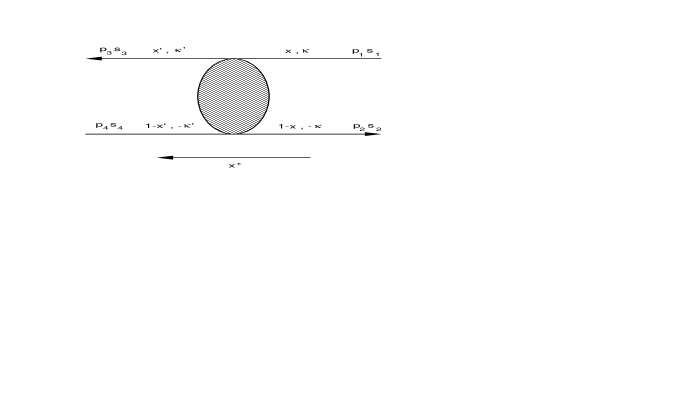
Figure 2: This illustrates the spin and momenta label conventions used for this positronium calculation.

Given this second-order interaction, the free matrix elements of $H_{\lambda}$, shown in Eq. (2), in the exchange and annihilation channels are

Exchange Channel:

$$V_{{}_{\lambda,exchange}} \equiv \frac{\langle e(3){\overline{e}}(4)|H_{\lambda}|e(1){\overline{e}}(2)\rangle|_{{}_{exchange}}}{16\pi^{3}\delta^{3}(p_{1}+p_{2}-p_{3}-p_{4})\sqrt{xx^{\prime}(1-x)(1-x^{\prime})}}$$ (16)

$$\equiv V_{1}+V_{2}+{\cal O}(e^{4})\;,$$

where

$$V_{1} = -\;e^{2}\;N_{1}\;\;\theta\left(\lambda^{2}-\left|{\cal M}_{0}^{2}-{{\cal M}_{0}^{\prime}}^{2}\right|\right)$$ (17)

$$\times\left(\frac{\theta\left(\left|\Delta_{1}\right|-\left|\Delta_{2}\right|\right)\theta\left(\left|\Delta_{1}\right|-\lambda^{2}\right)}{DEN_{1}}+\frac{\theta\left(\left|\Delta_{2}\right|-\left|\Delta_{1}\right|\right)\theta\left(\left|\Delta_{2}\right|-\lambda^{2}\right)}{DEN_{2}}\right)\;,~{}~{}$$

$$V_{2} = -\;e^{2}\;\theta\left(\lambda^{2}-\left|{\cal M}_{0}^{2}-{{\cal M}_{0}^{\prime}}^{2}\right|\right)\left(\frac{4}{(x-x^{\prime})^{2}}\delta_{s_{1}s_{3}}\delta_{s_{2}s_{4}}\right)\;.$$ (18)

The variables are defined as follows (see Figure 2 also):

$$\bullet\;\;p_{1} = \left(x{\cal P}^{+},\kappa+x{\cal P}^{\perp}\right)\;,\;p_{2}=\left((1-x){\cal P}^{+},-\kappa+(1-x){\cal P}^{\perp}\right)\;$$

$$\bullet\;\;p_{3} = \left(x^{\prime}{\cal P}^{+},\kappa^{\prime}+x^{\prime}{\cal P}^{\perp}\right)\;,\;p_{4}=\left((1-x^{\prime}){\cal P}^{+},-\kappa^{\prime}+(1-x^{\prime}){\cal P}^{\perp}\right)\;$$

$$\bullet\;\;N_{1} = \delta_{s_{1}s_{3}}\delta_{s_{2}s_{4}}T_{1}^{\perp}\cdot T_{2}^{\perp}-2m^{2}\delta_{s_{2}{\overline{s}_{4}}}\delta_{s_{2}{\overline{s}_{1}}}\delta_{s_{3}{\overline{s}_{1}}}\frac{(x-x^{\prime})^{2}}{xx^{\prime}(1-x)(1-x^{\prime})}$$

$$+ im\sqrt{2}(x^{\prime}-x)\left(\frac{s_{1}}{xx^{\prime}}\delta_{{\overline{s}_{1}}s_{3}}\delta_{s_{2}s_{4}}\epsilon_{s_{1}}^{\perp}\cdot T_{1}^{\perp}+\frac{s_{2}}{(1-x)(1-x^{\prime})}\delta_{{\overline{s}_{4}}s_{2}}\delta_{s_{1}s_{3}}\epsilon_{s_{2}}^{\perp}\cdot T_{2}^{\perp}\right)\;$$

$$\bullet\;\;T_{1}^{i} = -\frac{2(\kappa^{i}-{\kappa^{\prime}}^{i})}{x-x^{\prime}}-\frac{{\kappa^{\prime}}^{i}({\overline{s}_{2}})}{1-x^{\prime}}-\frac{\kappa^{i}(s_{2})}{1-x}\;,\;T_{2}^{i}=\frac{2(\kappa^{i}-{\kappa^{\prime}}^{i})}{x-x^{\prime}}-\frac{{\kappa^{\prime}}^{i}({\overline{s}_{1}})}{x^{\prime}}-\frac{\kappa^{i}(s_{1})}{x}$$

$$\bullet\;\;\kappa^{j}(s) = \kappa^{j}+i\;s\;\epsilon_{jk}\;\kappa^{k}\;\;(s\;=\;\pm\;1\;{\rm and}\;{\overline{s}}\equiv-s)\;\;;\epsilon_{12}=-\epsilon_{21}=1\;,\;\epsilon_{11}=\epsilon_{22}=0$$

$$\bullet\;\;\Delta_{1} = \frac{DEN_{1}}{x^{\prime}-x}\;,\;\Delta_{2}=\frac{DEN_{2}}{x^{\prime}-x}$$

$$\bullet\;\;DEN_{1} = \frac{(\kappa x^{\prime}-\kappa^{\prime}x)^{2}}{xx^{\prime}}+\frac{(mx-mx^{\prime})^{2}}{xx^{\prime}}\;,\;DEN_{2}=DEN_{1}|_{x\rightarrow 1-x\;,\;x^{\prime}\rightarrow 1-x^{\prime}}$$

$$\bullet\;\;{\cal M}_{0}^{2} = \frac{{\kappa}^{2}+m^{2}}{x(1-x)}\;,\;{{\cal M}_{0}^{\prime}}^{2}=\frac{{\kappa^{\prime}}^{2}+m^{2}}{x^{\prime}(1-x^{\prime})}\;.$$

Annihilation Channel:

$$V_{{}_{\lambda,annihil}} \equiv \frac{\langle e(3){\overline{e}}(4)|H_{\lambda}|e(1){\overline{e}}(2)\rangle|_{{}_{annihilation}}}{16\pi^{3}\delta^{3}(p_{1}+p_{2}-p_{3}-p_{4})\sqrt{xx^{\prime}(1-x)(1-x^{\prime})}}$$ (19)

$$\equiv V_{3}+V_{4}+{\cal O}(e^{4})\;,$$

where

$$V_{3}=\;e^{2}\;N_{2}\;\;\theta\left(\lambda^{2}-\left|{\cal M}_{0}^{2}-{{\cal M}_{0}^{\prime}}^{2}\right|\right)\left(\frac{\theta\left({\cal M}_{0}^{2}-{{\cal M}_{0}^{\prime}}^{2}\right)\theta\left({\cal M}_{0}^{2}-\lambda^{2}\right)}{{\cal M}_{0}^{2}}\right.$$

$$~{}~{}~{}~{}~{}~{}~{}~{}~{}~{}~{}~{}~{}~{}~{}~{}~{}~{}~{}~{}~{}~{}~{}~{}~{}~{}~{}~{}~{}~{}~{}~{}~{}~{}~{}~{}~{}~{}~{}~{}~{}~{}+\left.\frac{\theta\left({{\cal M}_{0}^{\prime}}^{2}-{\cal M}_{0}^{2}\right)\theta\left({{\cal M}_{0}^{\prime}}^{2}-\lambda^{2}\right)}{{{\cal M}_{0}^{\prime}}^{2}}\right)~{},$$ (20)

$$V_{4}=\;4e^{2}\theta\left(\lambda^{2}-\left|{\cal M}_{0}^{2}-{{\cal M}_{0}^{\prime}}^{2}\right|\right)\delta_{s_{1}{\overline{s}_{2}}}\delta_{s_{3}{\overline{s}_{4}}}\;,$$ (21)

and

$$\;\;N_{2} = \delta_{s_{1}{\overline{s}_{2}}}\delta_{s_{4}{\overline{s}_{3}}}T_{3}^{\perp}\cdot T_{4}^{\perp}+\delta_{s_{1}s_{2}}\delta_{s_{1}s_{4}}\delta_{s_{3}s_{4}}\frac{2m^{2}}{xx^{\prime}(1-x)(1-x^{\prime})}$$

$$~{}~{}~{}~{}+im\sqrt{2}\left(\frac{s_{1}}{x(1-x)}\delta_{s_{1}s_{2}}\delta_{s_{4}{\overline{s}_{3}}}\epsilon_{s_{1}}^{\perp}\cdot T_{3}^{\perp}-\frac{s_{4}}{x^{\prime}(1-x^{\prime})}\delta_{s_{1}{\overline{s}_{2}}}\delta_{s_{3}s_{4}}{\epsilon_{s_{4}}^{\perp}}^{\ast}\cdot T_{4}^{\perp}\right)\;,$$

$$\;\;T_{3}^{i} = \frac{{\kappa^{\prime}}^{i}(s_{3})}{1-x^{\prime}}-\frac{{\kappa^{\prime}}^{i}({\overline{s}_{3}})}{x^{\prime}}\;,\;T_{4}^{i}=\frac{{\kappa}^{i}({\overline{s}_{1}})}{1-x}-\frac{{\kappa}^{i}(s_{1})}{x}\;.$$

$V_{2}$ and $V_{4}$ are canonical instantaneous exchange and annihilation interactions, respectively, with widths restricted by the regulating function, $f_{\lambda}$. $V_{1}$ and $V_{3}$ are effective interactions that arise because photon emission and annihilation have vertices with widths restricted by the regulating function, $f_{\lambda}$.

2 Diagonalization of $H_{\lambda}$

First we discuss the lowest order spectrum of $H_{\lambda}$, after which we discuss BSPT, renormalization and a limiting procedure which allows the effects of low-energy (energy transfer below $\lambda$) emission to be transferred to the $|e{\overline{e}}\rangle$ sector alone.

1 ${\cal H}_{0}$, a coordinate change and its exact spectrum

${\cal H}_{0}$, as motivated from the form of our second-order effective Hamiltonian, in the $|e{\overline{e}}\rangle$ sector is

$${\cal H}_{0} = h+{\cal V}_{{}_{C}}\;,$$ (22)

where $h$ is the free Hamiltonian given in Eq. (12), and ${\cal V}_{{}_{C}}$ is given by [using the same variables defined below Eq. (18); note, $\kappa_{z}$ is defined below by Eq. (24)]

$$\frac{\langle e(3){\overline{e}}(4)|{\cal V}_{{}_{C}}|e(1){\overline{e}}(2)\rangle}{16\pi^{3}\delta^{3}(p_{1}+p_{2}-p_{3}-p_{4})\sqrt{xx^{\prime}(1-x)(1-x^{\prime})}}\equiv V_{{}_{C}}\;,$$

$$\hskip 72.26999pt{\rm where}~{}~{}~{}~{}~{}V_{{}_{C}}\equiv-\frac{16m^{2}e^{2}\delta_{s_{1}s_{3}}\delta_{s_{2}s_{4}}}{(\kappa-\kappa^{\prime})^{2}+(\kappa_{z}-\kappa_{z}^{\prime})^{2}}\;.$$ (23)

In all other sectors, we choose ${\cal H}_{0}=h$. This is convenient for the leading order spin-splitting calculation (order $\alpha^{4}$) in positronium, but for example in the Lamb shift calculation it is more convenient to keep the Coulomb interaction between the oppositely charged valence particles to all orders in all sectors.

As already mentioned, ${\cal H}_{0}$ in the $|e{\overline{e}}\rangle$ sector is motivated from the form of our second order effective Hamiltonian $H_{\lambda}$: it arises as the leading order term in a nonrelativistic limit of the instantaneous photon exchange interaction combined with the two time-orderings of the dynamical photon exchange interaction. We choose it to simplify positronium bound-state calculations. Other choices are possible, and must be used to study problems such as photon emission. Later, in BSPT this choice is shown to produce the leading order contribution to positronium’s binding-energy (order $\alpha^{2}$) as long as $m\alpha^{2}\ll\tilde{\lambda}\ll m\alpha$.

The coordinates $\kappa_{z}$ and $\kappa_{z}^{\prime}$ in Eq. (23) follow from a standard coordinate transformation that takes the range of longitudinal momentum fraction, $x\in[0,1]$ to $\kappa_{z}\in[-\infty,\infty]$. This coordinate change is

$$x \equiv \frac{1}{2}+\frac{\kappa_{z}}{2\sqrt{\kappa^{2}+\kappa_{z}^{2}+m^{2}}}\;.$$ (24)

We introduce a new three-vector

$${\bf p} \equiv (\kappa,\kappa_{z})\;.$$ (25)

Note that

$${\cal M}_{0}^{2} \equiv \frac{\kappa^{2}+m^{2}}{x(1-x)}=4(m^{2}+{\bf p}^{2})$$ (26)

is invariant with respect to rotations in the space of vectors ${\bf p}$. The nonrelativistic kinematics of Eqs. (2) and (3) in terms of this three-vector become

$$\frac{|{\bf p}|}{m} = {\cal O}(\alpha)\;.$$ (27)

Note the simple forms that our “exchange channel denominators” take in the nonrelativistic limit

$$DEN_{1} = ({\bf p}-{\bf p}^{\prime})^{2}-\frac{(\kappa_{z}-\kappa_{z}^{\prime})({\bf p}^{2}-{{\bf p}^{\prime}}^{2})}{m}+{\cal O}\left[\left(\frac{{\bf p}}{m}\right)^{5}m^{2}\right]~{},$$ (28)

$$DEN_{2} = ({\bf p}-{\bf p}^{\prime})^{2}+\frac{(\kappa_{z}-\kappa_{z}^{\prime})({\bf p}^{2}-{{\bf p}^{\prime}}^{2})}{m}+{\cal O}\left[\left(\frac{{\bf p}}{m}\right)^{5}m^{2}\right]~{}.$$ (29)

Also note the form that the longitudinal momentum fraction transferred between the electron and positron takes

$$x-x^{\prime} = \frac{\kappa_{z}-\kappa_{z}^{\prime}}{2m}+\frac{({{\bf p}^{\prime}}^{2}\kappa_{z}^{\prime}-{\bf p}^{2}\kappa_{z})}{4m^{3}}+{\cal O}\left[\left(\frac{{\bf p}}{m}\right)^{5}\right]\;.$$ (30)

These formulas are consistently used throughout this chapter.

Now we describe the leading Schrödinger equation. We seek solutions of the following eigenvalue equation

$${\cal H}_{0}|\psi_{N}({\cal P})\rangle = {\cal E}_{N}|\psi_{N}({\cal P})\rangle\;,$$ (31)

where ${\cal E}_{N}\equiv\frac{{{\cal P}^{\perp}}^{2}+{\cal M}_{N}^{2}}{{\cal P}^{+}}$. ${\cal H}_{0}$ is diagonal with respect to the different particle sectors, thus we can solve Eq. (31) sector by sector. In all sectors other than $|e{\overline{e}}\rangle$, ${\cal H}_{0}=h$, and the solution is trivial. For the $|e{\overline{e}}\rangle$ sector, a general $|\psi_{N}({\cal P})\rangle$ is

$$|\psi_{N}({\cal P})\rangle = \sum_{s_{1}s_{2}}\int_{p_{1}p_{2}}\sqrt{p_{1}^{+}p_{2}^{+}}16\pi^{3}\delta^{3}({\cal P}-p_{1}-p_{2})$$ (32)

$$~{}~{}~{}~{}~{}~{}~{}~{}\times\;{\tilde{\phi}}_{N}(x\kappa s_{1}s_{2})~{}b_{s_{1}}^{\dagger}(p_{1})\;d_{s_{2}}^{\dagger}(p_{2})\;|0\rangle\;,$$

with norm

$$\langle\psi_{N}({\cal P})|\psi_{N^{\prime}}({\cal P}^{\prime})\rangle\equiv\delta_{NN^{\prime}}16\pi^{3}{\cal P}^{+}\delta^{3}\left({\cal P}-{\cal P}^{\prime}\right)$$

$$\Longrightarrow\;\sum_{s_{1}s_{2}}\frac{\int d^{2}\kappa\int_{0}^{1}dx}{16\pi^{3}}{{\tilde{\phi}}_{N}}^{\ast}(x\kappa s_{1}s_{2}){\tilde{\phi}}_{N^{\prime}}(x\kappa s_{1}s_{2})\;=\;\delta_{NN^{\prime}}\;.$$

The tilde on ${\tilde{\phi}}_{N}$ will be notationally convenient below. In the $|e{\overline{e}}\rangle$ sector, Eq. (31) becomes

$$\left({\cal M}_{{}_{N}}^{2}-\frac{{\kappa^{\prime}}^{2}+m^{2}}{x^{\prime}(1-x^{\prime})}\right){\tilde{\phi}}_{N}(x^{\prime}\kappa^{\prime}s_{3}s_{4})=\sum_{s_{1}s_{2}}\frac{\int d^{2}\kappa\int_{0}^{1}dx}{16\pi^{3}}~{}V_{{}_{C}}~{}{\tilde{\phi}}_{N}(x\kappa s_{1}s_{2})\;.$$ (33)

After the above coordinate change, this becomes [J(p) is the Jacobian of the coordinate change written below]

$$\left[{\cal M}_{{}_{N}}^{2}-4(m^{2}+{{\bf p}^{\prime}}^{2})\right]\phi_{N}({\bf p}^{\prime}s_{3}s_{4})=\sum_{s_{1}s_{2}}\int\frac{d^{3}p\sqrt{J(p)J(p^{\prime})}}{16\pi^{3}}~{}V_{{}_{C}}~{}\phi_{N}({\bf p}s_{1}s_{2})\;,~{}~{}~{}~{}$$ (34)

where the tilde on the wavefunction has been removed by redefining the norm in a convenient fashion

$$\delta_{NN^{\prime}} = \sum_{s_{1}s_{2}}\frac{\int d^{2}\kappa\int_{0}^{1}dx}{16\pi^{3}}{{\tilde{\phi}}_{N}}^{\ast}(x\kappa s_{1}s_{2}){\tilde{\phi}}_{N^{\prime}}(x\kappa s_{1}s_{2})=\sum_{s_{1}s_{2}}\int d^{3}p\frac{J(p)}{16\pi^{3}}{{\tilde{\phi}}_{N}}^{\ast}({\bf p}s_{1}s_{2}){\tilde{\phi}}_{N^{\prime}}({\bf p}s_{1}s_{2})$$ (35)

$$\equiv \sum_{s_{1}s_{2}}\int d^{3}p\;\phi_{N}^{\ast}({\bf p}s_{1}s_{2})\phi_{N^{\prime}}({\bf p}s_{1}s_{2})\;,$$

and the Jacobian of the coordinate change is

$$J(p) \equiv \frac{dx}{d\kappa_{z}}=\frac{\kappa^{2}+m^{2}}{2({\bf p}^{2}+m^{2})^{\frac{3}{2}}}\;.$$ (36)

Note that the Jacobian factor in Eq. (34) satisfies

$$\sqrt{J(p)J(p^{\prime})} = \frac{1}{2m}\left[1-\frac{{\bf p}^{2}+2\kappa_{z}^{2}+{{\bf p}^{\prime}}^{2}+2{\kappa_{z}^{\prime}}^{2}}{4m^{2}}+{\cal O}\left(\frac{{\bf p}^{4}}{m^{4}},\frac{{{\bf p}^{\prime}}^{4}}{m^{4}},\cdots\right)\right]\;.$$ (37)

Before defining ${\cal H}_{0}$ in the $|e{\overline{e}}\rangle$ sector we mention a subtle but important point in the definition of ${\cal H}_{0}$. ${\cal H}_{0}$ in the $|e{\overline{e}}\rangle$ sector will not be defined by Eq. (34). Rather, it will be defined by taking the leading order nonrelativistic expansion of the Jacobian factor in Eq. (34). This gives

$$\left[{\cal M}_{{}_{N}}^{2}-4(m^{2}+{{\bf p}^{\prime}}^{2})\right]\phi_{N}({\bf p}^{\prime}s_{3}s_{4}) = \sum_{s_{1}s_{2}}\int\frac{d^{3}p\left(\frac{1}{2m}\right)}{16\pi^{3}}~{}V_{{}_{C}}~{}\phi_{N}({\bf p}s_{1}s_{2})\;,$$ (38)

where $V_{{}_{C}}$ is defined in Eq. (23). This ${\cal H}_{0}$ will be diagonalized exactly, and the subsequent BSPT will be set up as an expansion in ${\cal V}\equiv H_{\lambda}-{\cal H}_{0}$, which will then be regrouped in terms of a consistent expansion in $\alpha$ and $\alpha\ln(1/\alpha)$ to some prescribed order. First, we discuss the exact diagonalization of ${\cal H}_{0}$.

Putting the expression for $V_{{}_{C}}$ into Eq. (38) results in the following equation

$$\left(-{\cal B}_{{}_{N}}+\frac{{{\bf p}^{\prime}}^{2}}{m}\right)\phi_{N}({\bf p}^{\prime}s_{3}s_{4}) = \frac{\alpha}{2\pi^{2}}\int\frac{d^{3}p}{({\bf p}-{\bf p}^{\prime})^{2}}\phi_{N}({\bf p}s_{3}s_{4})\;.$$ (39)

This is recognized as the familiar nonrelativistic Schrödinger equation for positronium. Note that we have defined a leading order binding-energy, $-{\cal B}_{N}$, as

$${\cal M}_{N}^{2} \equiv 4m^{2}+4m{\cal B}_{{}_{N}}\;,$$ (40)

where ${\cal M}_{N}^{2}$ is the leading order mass-squared. Note the difference in the definition of our leading order binding-energy and our exact binding-energy as given by $M_{{}_{N}}^{2}\equiv(2m+B_{{}_{N}})^{2}$ [see Appendix 10 for further discussion on this difference], where $M_{N}^{2}$ is the exact mass-squared.

To proceed with the solution of Eq. (39) note that there is no spin dependence in the operator so the spin part just factors out

$$\phi_{\nu,s_{e},s_{{}_{{\overline{e}}}}}({\bf p}^{\prime}s_{3}s_{4}) \equiv \phi_{\nu}({\bf p}^{\prime})\delta_{s_{e}s_{3}}\delta_{s_{{}_{{\overline{e}}}}s_{4}}\;.$$ (41)

We rewrote $N$ as $(\nu,s_{e},s_{{}_{{\overline{e}}}})$, where $(s_{e},s_{{}_{{\overline{e}}}})$ label the spin quantum numbers and $\nu$ labels all other quantum numbers, which are discrete for the bound states and continuous for the scattering states.

The solutions to Eq. (39) are well known. For ${\cal B}_{{}_{N}}<0$, following Fock [39], we change coordinates according to

$$m{\cal B}_{{}_{N}} \equiv -e_{n}^{2}~{},$$ (42)

$$u \equiv (u_{0},{\bf u})~{},$$ (43)

$$u_{0} \equiv \cos(\omega)\equiv\frac{e_{n}^{2}-{\bf p}^{2}}{e_{n}^{2}+{\bf p}^{2}}~{},$$ (44)

$${\bf u} \equiv \frac{{\bf p}}{p}\sin(\omega)\equiv\sin(\omega)\left[\sin(\theta)\cos(\phi),sin(\theta)\sin(\phi),\cos(\theta)\right]$$ (45)

$$\equiv \frac{2e_{n}{\bf p}}{e_{n}^{2}+{\bf p}^{2}}\;.$$

Useful relations implied by this coordinate change are in Appendix 9. Note that in our notation we anticipate that $\nu$ will be given by $(n,l,m_{{}_{l}})$, the usual principal and angular momentum quantum numbers, and that the leading order binding-energy will depend only on the principal quantum number, $n$. Given this, Eq. (39) becomes

$$\psi_{\nu}(\Omega_{p^{\prime}}) \equiv \frac{\alpha}{2\pi^{2}}\frac{m}{2e_{n}}\int\frac{d\Omega_{p}}{|u-u^{\prime}|^{2}}\psi_{\nu}(\Omega_{p})\;,$$ (46)

where

$$\psi_{\nu}(\Omega_{p}) \equiv \frac{(e_{n}^{2}+{\bf p}^{2})^{2}}{4(e_{n})^{\frac{5}{2}}}\phi_{\nu}({\bf p})\;.$$ (47)

Using Eq. (20) of Appendix 9, this is seen to have the following solution:

$$\psi_{\nu}(\Omega_{p})=Y_{\nu}(\Omega_{p})~{}~{}{\rm with}~{}~{}\frac{\alpha}{2\pi^{2}}\frac{m}{2e_{n}}\frac{2\pi^{2}}{n}=1\;,$$ (48)

where $Y_{\nu}(\Omega_{p})$ is a hyperspherical harmonic. Thus,

$$e_{n}=\frac{m\alpha}{2n}~{}\Longrightarrow~{}{\cal B}_{{}_{N}}=-\frac{m\alpha^{2}}{4n^{2}}\;,$$ (49)

and

$$\phi_{\nu}({\bf p})=\frac{4(e_{n})^{\frac{5}{2}}}{(e_{n}^{2}+{\bf p}^{2})^{2}}Y_{\nu}(\Omega_{p})\;.$$ (50)

This is the standard nonrelativistic solution for the bound states of positronium. This completes the solution of ${{\cal H}}_{0}$ for the bound-states. The scattering states are also needed in our second-order BSPT calculation. We use Green’s function techniques to include the scattering states where required.

2 BSPT, renormalization and a limit

Here we use the BSPT formulas (appropriately generalized to the degenerate case) of Section 3 to analyze positronium’s leading ground state spin splitting. The potential to be used in BSPT is

$${\cal V} = H_{\lambda}-{\cal H}_{0}\;,$$ (51)

where the eigenvalue equation for ${\cal H}_{0}$ is given by Eq. (38), and $H_{\lambda}$ to second order is given in Section 1. We will be perturbing about the nonperturbative eigenstates of ${\cal H}_{0}$.

First, we discuss electron mass renormalization. In second-order BSPT there is an electron mass shift coming from the $f_{\lambda}v$ part of $H_{\lambda}$, with $v$ given by $\int d^{2}x^{\perp}dx^{-}{\cal H}_{ee\gamma}$ [see Eq. (53)]. This is photon emission and absorption restricted by the regulating function, $f_{\lambda}$. The calculation is similar to that of Subsection 1. Assuming $\langle{\cal M}_{{}_{N}}^{2}-{\cal M}_{0}^{2}\rangle={\cal O}(e^{2})$, this electron mass-squared shift is

$$\delta m^{2} = -\delta\Sigma_{\lambda}^{{}^{(2)}}+{\cal O}(e^{4})\;.$$ (52)

$\delta\Sigma_{\lambda}^{{}^{(2)}}$ is the same function that was defined in Eq. (9). Checking the consistency: using this result [Eq. (52)] one obtains $\langle{\cal M}_{{}_{N}}^{2}-{\cal M}_{0}^{2}\rangle=\langle 4m^{2}+4m{\cal B}_{{}_{N}}-4(m^{2}+{\bf p}^{2})\rangle={\cal O}(e^{4})$, and our initial assumption is satisfied. Combining this with the coherent electron mass-squared $m_{\lambda}^{2}$ of Eq. (12), the physical electron mass-squared $m_{phys}^{2}$ through second-order is

$$m_{phys}^{2} = m_{\lambda}^{2}+\delta m^{2}$$ (53)

$$= \left[m^{2}-\left(\delta\Sigma_{\Lambda}^{{}^{(2)}}-\delta\Sigma_{\lambda}^{{}^{(2)}}\right)+\delta v_{\Lambda}^{{}^{(2)}}\right]+\left[-\delta\Sigma_{\lambda}^{{}^{(2)}}\right]+{\cal O}(e^{4})$$

$$= m^{2}+{\cal O}(e^{4})\;.$$

In this last step we recalled the result from coupling coherence of Eq. (11). We see that through second order, the physical electron mass is equivalent to the renormalized electron mass in the free Hamiltonian $h$. As already mentioned, we see that our choice of renormalization prescription mentioned in footnote 3 corresponds to a physical prescription as the physical electron mass is equivalent to the renormalized electron mass through second order. Of course we do not have to use this physical prescription, but it is our choice here, and must be maintained consistently in higher order calculations. As promised below Eq. (12), we see that treating photons perturbatively has led to an exact cancellation of the infrared divergence in the coherent electron mass-squared $m_{\lambda}^{2}$, and the physical electron mass through second-order is infrared finite.

Now we move on to the discussion of BSPT. The only channels to order $e^{2}$ are exchange and annihilation. Parts of these effective interactions are given in Subsection 2. We also need to include the perturbative mixing of the $|e{\overline{e}}\gamma\rangle$ and $|\gamma\rangle$ sectors with the $|e{\overline{e}}\rangle$ sector arising from $f_{\lambda}v$, with $v=\int d^{2}x^{\perp}dx^{-}{\cal H}_{ee\gamma}$. In second-order BSPT this gives rise to the following effective interactions that must be added to $V_{{}_{\lambda,exchange}}$ and $V_{{}_{\lambda,annihil}}$ of Eqs. (16) and (19) respectively.

Exchange Channel:

$$V_{5} = \frac{-e^{2}N_{1}\theta\left(\lambda^{2}-\left|\Delta_{1}\right|\right)\theta\left(\lambda^{2}-\left|\Delta_{2}\right|\right)}{DEN_{3}}\;,$$ (54)

with

$$DEN_{3} = (\kappa-\kappa^{\prime})^{2}+\frac{1}{2}(x-x^{\prime})A+|x-x^{\prime}|\left(\frac{1}{2}\left({\cal M}_{0}^{2}+{{\cal M}_{0}^{\prime}}^{2}\right)-{\cal M}_{{}_{N}}^{2}\right)\;,$$

and

$$A = \frac{\kappa^{2}+m^{2}}{1-x}-\frac{{\kappa^{\prime}}^{2}+m^{2}}{1-x^{\prime}}+\frac{{\kappa^{\prime}}^{2}+m^{2}}{x^{\prime}}-\frac{\kappa^{2}+m^{2}}{x}\;.$$

Annihilation Channel:

$$V_{6} = \;e^{2}\;N_{2}\;\;\frac{\theta\left(\lambda^{2}-{\cal M}_{0}^{2}\right)\theta\left(\lambda^{2}-{{\cal M}_{0}^{\prime}}^{2}\right)}{{\cal M}_{{}_{N}}^{2}}\;.$$ (55)

Note that in a nonrelativistic expansion [after the coordinate change of Eq. (24)] the above “exchange channel denominator” becomes

$$DEN_{3}=({\bf p}-{\bf p}^{\prime})^{2}+|x-x^{\prime}|\left(\frac{1}{2}\left({\cal M}_{0}^{2}+{{\cal M}_{0}^{\prime}}^{2}\right)-{\cal M}_{{}_{N}}^{2}\right)+{\cal O}\left[\left(\frac{{\bf p}}{m}\right)^{6}m^{2}\right]\;.~{}~{}~{}$$ (56)

The full exchange and annihilation channel interactions to order $e^{2}$ are

$$V_{{}_{exchange}} \equiv V_{{}_{\lambda,exchange}}+V_{5}\;,$$ (57)

$$V_{{}_{annihil}} \equiv V_{{}_{\lambda,annihil}}+V_{6}\;,$$ (58)

where Eqs. (16) and (19) give $V_{{}_{\lambda,exchange}}$ and $V_{{}_{\lambda,annihil}}$ respectively.

One way to summarize the results, recalling the form of Eq. (34) and the norm in Eq. (35), is to state: The full order $e^{2}$ effective interactions give rise to the following first order BSPT shift of the bound-state mass-squared spectrum of ${\cal H}_{0}$

$$\delta^{{}^{(1)}}M^{2}(s_{3},s_{4};s_{1},s_{2})\equiv\langle\phi_{n,l,m_{l},s_{3},s_{4}}|V|\phi_{n,l,m_{l},s_{1},s_{2}}\rangle$$

$$~{}~{}~{}~{}~{}~{}=\int d^{3}p~{}d^{3}p^{\prime}\phi_{n,l,m_{l}}^{\ast}({\bf p}^{\prime})V({\bf p}^{\prime},s_{3},s_{4};{\bf p},s_{1},s_{2})\phi_{n,l,m_{l}}({\bf p})\;,$$ (59)

where

$$V({\bf p}^{\prime},s_{3},s_{4};{\bf p},s_{1},s_{2}) = \sqrt{\frac{J(p)}{16\pi^{3}}\frac{J(p^{\prime})}{16\pi^{3}}}\left(V_{{}_{exchange}}+V_{{}_{annihil}}\right)$$ (60)

$$~{}~{}~{}~{}~{}~{}~{}~{}~{}~{}~{}~{}~{}~{}~{}~{}~{}~{}~{}-\sqrt{\frac{\left(\frac{1}{2m}\right)}{16\pi^{3}}\frac{\left(\frac{1}{2m}\right)}{16\pi^{3}}}\left(V_{{}_{C}}\right)\;.$$

The Dirac notation in Eq. (59) will be used in the remainder of this chapter. See Eqs. (23), (57) and (58) for $V_{{}_{C}}$, $V_{{}_{exchange}}$ and $V_{{}_{annihil}}$ respectively. The interaction $V$ must be diagonalized in the degenerate spin space following the standard rules of degenerate BSPT. Note that in order to get all the shifts through a consistent order in $\alpha$ (in this case through order $\alpha^{4}$), $V$ needs to be considered in second order BSPT also.

The diagonalization of $V$ in the degenerate spin space follows shortly, but first we determine the range of $\lambda$ that allows the effects of low-energy (energy transfer below $\lambda$) photon emission and absorption to be transferred to the effective interactions in the $|e{\overline{e}}\rangle$ sector alone, and at the same time does not remove the nonperturbative bound-state physics of interest. This range is

$$\frac{\left|M_{N}^{2}-(2m)^{2}\right|}{{\cal P}^{+}}\ll\frac{\lambda^{2}}{{\cal P}^{+}}\ll q^{-}_{{}_{photon}}\;,$$ (61)

where $M_{N}^{2}$ is the bound-state mass-squared and $q^{-}_{{}_{photon}}$ is the dominant energy of an emitted photon. After the solutions of ${\cal H}_{0}$ are known the $\alpha$-scaling in all BSPT matrix elements is known and the bounds in Eq. (61) become

$$m^{2}\alpha^{2}\ll\lambda^{2}\ll m^{2}\alpha\;.$$ (62)

This is satisfied under the following limit

$$\lambda^{2}\; \longrightarrow {\rm a\;fixed\;number}~{},$$ (63)

$$\frac{m^{2}\alpha^{2}}{\lambda^{2}} \longrightarrow 0~{},$$ (64)

$$\frac{m^{2}\alpha}{\lambda^{2}} \longrightarrow \infty\;.$$ (65)

Given the nonrelativistic limit

$$\alpha \longrightarrow 0~{},$$ (66)

$$\frac{m^{2}}{\lambda^{2}} \longrightarrow \infty\;,$$ (67)

this implies

$$\frac{m^{2}}{\lambda^{2}}\propto\alpha^{-\frac{k}{2}}\;,$$ (68)

with

$$2<k<4~{}~{}.$$ (69)

Note that this “window of opportunity” is available to us because, (i) we have an adjustable effective cutoff $\frac{\lambda^{2}}{{\cal P}^{+}}$ in the theory, and (ii) QED is a theory with two dynamical energy scales, $\frac{m^{2}\alpha^{2}}{{\cal P}^{+}}$ and $\frac{m^{2}\alpha}{{\cal P}^{+}}$, a fact known for a long time, and the reason that QED calculations have been so successful over the years.

Given the above limit [Eqs. (63)–(65)],

$$\bullet \theta\left(\lambda^{2}-4|{\bf p}^{2}-{{\bf p}^{\prime}}^{2}|\right),\theta\left(|\Delta_{1}|-\lambda^{2}\right),\theta\left(|\Delta_{2}|-\lambda^{2}\right)\longrightarrow 1$$ (70)

$$\bullet \theta\left(4({\bf p}^{2}+m^{2})-\lambda^{2}\right),\theta\left(4({{\bf p}^{\prime}}^{2}+m^{2})-\lambda^{2}\right)\longrightarrow 1$$ (71)

$$\bullet \theta\left(\lambda^{2}-|\Delta_{1}|\right),\theta\left(\lambda^{2}-|\Delta_{2}|\right)\longrightarrow 0$$ (72)

$$\bullet \theta\left(\lambda^{2}-4({\bf p}^{2}+m^{2})\right),\theta\left(\lambda^{2}-4({{\bf p}^{\prime}}^{2}+m^{2})\right)\longrightarrow 0\;.$$ (73)

Now we proceed with the diagonalization of $V$ in the degenerate spin space [see Eqs. (59) and (60)]. In BSPT with $V$ we will calculate all corrections through order $\alpha^{4}$ that give rise to a spin splitting structure in the ground state of ${\cal H}_{0}$. First, we write the general $V$ more explicitly given the above limits in Eqs. (70)–(73):

$$V({\bf p}^{\prime},s_{3},s_{4};{\bf p},s_{1},s_{2}) = \frac{1}{16\pi^{3}}\frac{1}{2m}\left[1-\frac{{\bf p}^{2}+2\kappa_{z}^{2}+{{\bf p}^{\prime}}^{2}+2{\kappa_{z}^{\prime}}^{2}}{4m^{2}}+{\cal O}\left(\frac{{\bf p}^{4}}{m^{4}}\right)\right]$$ (74)

$$\times \left(-\frac{e^{2}N_{1}}{DEN_{4}}-\frac{4e^{2}}{(x-x^{\prime})^{2}}\delta_{s_{1}s_{3}}\delta_{s_{2}s_{4}}+\frac{e^{2}N_{2}}{DEN_{5}}+4e^{2}\delta_{s_{1}{\overline{s}}_{2}}\delta_{s_{3}{\overline{s}}_{4}}\right)$$

$$- \frac{1}{16\pi^{3}}\frac{1}{2m}V_{{}_{C}}\;,$$

where

$$\bullet \frac{1}{DEN_{4}}\equiv\frac{\theta_{12}}{DEN_{1}}+\frac{\theta_{21}}{DEN_{2}}\;\;,\;\theta_{12}\equiv\theta\left(DEN_{1}-DEN_{2}\right)$$ (75)

$$\bullet \frac{1}{DEN_{5}}\equiv\frac{\theta\left({\cal M}_{0}^{2}-{{\cal M}_{0}^{\prime}}^{2}\right)}{{\cal M}_{0}^{2}}+\frac{\theta\left({{\cal M}_{0}^{\prime}}^{2}-{{\cal M}_{0}}^{2}\right)}{{{\cal M}_{0}^{\prime}}^{2}}\;.$$ (76)

Note that we have expanded out the Jacobian factors according to Eq. (37). Also, $DEN_{1}$ and $DEN_{2}$ are defined below Eq. (18) and written in their expanded version in Eqs. (28) and (29) respectively. Finally, $N_{1}$ and $N_{2}$ are written below Eqs. (18) and (21) respectively.

Since the eigenstate wavefunctions of ${\cal H}_{0}$ force ${\bf p}$ to scale as ${\bf p}\sim m\alpha$, it is useful to note the $\alpha$-scaling of the matrix elements of $V$ in momentum space in a nonrelativistic expansion. Recalling that we are always assuming $\alpha\longrightarrow 0$ (without which our matrix elements would not have a well-defined $\alpha$ scaling), we see the following structure arising

$$V = V^{{}^{(0)}}+V^{{}^{(1)}}+V^{{}^{(2)}}+\cdots\;,$$ (77)

where a momentum space matrix element of $V^{{}^{(S)}}$ scales as $V^{{}^{(S)}}\!\!\!\sim\alpha^{S}$. Thus in first-order BSPT these respective terms scale as (this follows noting $\int d^{3}p\left|\phi_{N}(p)\right|^{2}~{}=~{}1$ and $V$ is not diagonal in momentum space)

$$\delta^{{}^{(1)}}M_{NN^{\prime}}^{2}=\langle\phi_{N}|V^{{}^{(S)}}|\phi_{N^{\prime}}\rangle\sim\alpha^{3+S}\;.$$ (78)

To be consistent through order $\alpha^{4}$ in first-order BSPT we need to look at all the matrix elements of $V^{{}^{(S)}}$ with $S\leq 1$; and in second-order BSPT, since $\left|{\cal M}_{1}^{2}-{\cal M}_{n}^{2}\right|\sim m^{2}\alpha^{2}$, we need to consider $V^{{}^{(0)}}$ in second-order BSPT (since $\alpha^{3}\alpha^{3}/\alpha^{2}=\alpha^{4}$).

A final discussion that we must have, before we write out these expressions for $V^{{}^{(S)}}$, is how we are going to deal with $DEN_{4}$ and $DEN_{5}$ defined above. These denominators are dealt with by noting the following formulas

$$\frac{\theta(a-b)}{a}+\frac{\theta(b-a)}{b} = \frac{1}{2}\frac{\theta(a-b)+\theta(b-a)}{a}+\frac{1}{2}\frac{\theta(a-b)+\theta(b-a)}{b}$$ (79)

$$+ \frac{1}{2}\frac{\theta(a-b)-\theta(b-a)}{a}-\frac{1}{2}\frac{\theta(a-b)-\theta(b-a)}{b}$$

$$= \frac{1}{2}\left(\frac{1}{a}+\frac{1}{b}\right)+\frac{1}{2}\left[\theta(a-b)-\theta(b-a)\right]\left(\frac{1}{a}-\frac{1}{b}\right)$$

$$= \frac{1}{2}\left(\frac{1}{a}+\frac{1}{b}\right)+\frac{1}{2}\frac{\left|a-b\right|}{a-b}\left(\frac{1}{a}-\frac{1}{b}\right)$$

$$= \frac{1}{2}\left(\frac{1}{a}+\frac{1}{b}\right)-\frac{1}{2}\frac{\left|a-b\right|}{a~{}b}\;.$$

To proceed it is useful to note

$$DEN_{1}=({\bf p}-{\bf p}^{\prime})^{2}-\frac{(\kappa_{z}-\kappa_{z}^{\prime})({\bf p}^{2}-{{\bf p}^{\prime}}^{2})}{m}+{\cal O}\left[\left(\frac{{\bf p}}{m}\right)^{5}m^{2}\right]~{},$$ (80)

$$DEN_{1}=DEN_{2}-\frac{2(\kappa_{z}-\kappa_{z}^{\prime})({\bf p}^{2}-{{\bf p}^{\prime}}^{2})}{m}+{\cal O}\left[\left(\frac{{\bf p}}{m}\right)^{5}m^{2}\right]~{},$$ (81)

$$\frac{1}{2}\left(\frac{1}{DEN_{1}}+\frac{1}{DEN_{2}}\right)=\frac{1}{({\bf p}-{{\bf p}^{\prime}})^{2}}+$$

$$~{}~{}~{}~{}~{}~{}~{}~{}~{}~{}~{}~{}~{}~{}~{}~{}~{}~{}~{}~{}~{}~{}~{}~{}~{}~{}~{}~{}~{}~{}~{}~{}~{}~{}+\frac{(\kappa_{z}-\kappa_{z}^{\prime})^{2}({\bf p}^{2}-{{\bf p}^{\prime}}^{2})^{2}}{m^{2}({\bf p}-{\bf p}^{\prime})^{6}}+{\cal O}\left[\left(\frac{{\bf p}}{m}\right)^{2}\frac{1}{m^{2}}\right]\;.$$ (82)

Especially note that this last equation scales as: $\frac{1}{\alpha^{2}}+1+\alpha^{2}+\cdots$, i.e. the corrections start at order $1$ (not order $\frac{1}{\alpha}$); this implies that only the $\frac{1}{({\bf p}-{{\bf p}^{\prime}})^{2}}$ term of Eq. (82) contributes to the spin splittings to order $\alpha^{4}$. But we still have to discuss the second term that arises in Eq. (79). This term is given by

$$\left.\frac{1}{DEN_{4}}\right|_{{}_{second~{}term}}=-\frac{1}{2}\frac{\left|DEN_{1}-DEN_{2}\right|}{DEN_{1}DEN_{2}}=-\frac{1}{2}\frac{\left|\frac{2(\kappa_{z}-\kappa_{z}^{\prime})({\bf p}^{2}-{{\bf p}^{\prime}}^{2})}{m}\right|}{\left({\bf p}-{\bf p}^{\prime}\right)^{4}}+{\cal O}\left(\alpha^{0}\right)\;.~{}~{}~{}~{}$$ (83)

Including $N_{1}$, this starts out as an ${\cal O}(\alpha^{3})$ spin conserving contribution, which does not contribute to the splitting. The next order contribution is ${\cal O}(\alpha^{4})$ with spin structure, but is odd under ${\bf p}\leftrightarrow{\bf p}^{\prime}$, and thus integrates to zero in first-order BSPT (in second-order BSPT it contributes $\alpha^{4}\alpha^{4}/\alpha^{2}\sim\alpha^{6}$). However, the ${\cal O}(\alpha^{3})$ spin conserving term appears to lead to an order $\alpha^{4}$ shift to the spin splittings in second-order BSPT when the cross terms with $V^{{}^{(0)}}$ of Eq. (85) are considered; however, these cross term contributions add to zero due to the facts that the ${\cal O}(\alpha^{3})$ term including Eq. (83) conserves spin and the ${\cal O}(\alpha^{3})$ term including Eq. (83) is even while the term from Eq. (85) is odd under ${\bf p}\leftrightarrow{\bf p}^{\prime}$.

To summarize the preceding discussion of $DEN_{4}$ and $DEN_{5}$, we can say that through order $\alpha^{4}$, for the spin splittings of positronium, there are no relativistic corrections to the following replacements:

$$DEN_{4}\longrightarrow({\bf p}-{{\bf p}^{\prime}})^{2}~{}~{}{\rm and}~{}~{}DEN_{5}\longrightarrow 4m^{2}\;.$$ (84)

This is valid for the ground and excited states, but in what follows we specialize to the ground state for simplicity.

Given this general conclusion about $DEN_{4}$ and $DEN_{5}$, we list the pieces of $V$ that contribute to positronium’s ground state spin splittings through order $\alpha^{4}$. Explicitly, as far as the $\alpha$-scaling goes, we need to consider

$$V^{{}^{(0)}}({\bf p}^{\prime}s_{3}s_{4};{\bf p}s_{1}s_{2}) = \frac{-c_{{}_{ex}}e^{2}}{4\pi^{3}({\bf p}-{\bf p}^{\prime})^{2}}{v}^{(0)}({\bf p}^{\prime}s_{3}s_{4};{\bf p}s_{1}s_{2})\;,$$ (85)

where

$${v}^{(0)}({\bf p}^{\prime}s_{3}s_{4};{\bf p}s_{1}s_{2})\equiv\left[\delta_{s_{1}{\overline{s}}_{3}}\delta_{s_{2}s_{4}}f_{1}({\bf p}^{\prime}s_{3}s_{4};{\bf p}s_{1}s_{2})+\delta_{s_{1}s_{3}}\delta_{s_{2}{\overline{s}}_{4}}f_{2}({\bf p}^{\prime}s_{3}s_{4};{\bf p}s_{1}s_{2})\right],~{}~{}~{}~{}~{}~{}~{}$$ (86)

$$f_{1}({\bf p}^{\prime}s_{3}s_{4};{\bf p}s_{1}s_{2})\equiv s_{1}(\kappa_{y}-\kappa_{y}^{\prime})-i(\kappa_{x}-\kappa_{x}^{\prime})~{},$$ (87)

$$f_{2}({\bf p}^{\prime}s_{3}s_{4};{\bf p}s_{1}s_{2})\equiv s_{4}(\kappa_{y}-\kappa_{y}^{\prime})+i(\kappa_{x}-\kappa_{x}^{\prime})\;.$$ (88)

Recall that $s_{i}=\pm 1~{}(i=1,2,3,4)$ only. The only other interaction we need to consider is

$$V^{{}^{(1)}}({\bf p}^{\prime}s_{3}s_{4};{\bf p}s_{1}s_{2}) = \frac{e^{2}}{4m\pi^{3}}\left[c_{{}_{an}}\delta_{s_{1}s_{2}}\delta_{s_{1}s_{4}}\delta_{s_{3}s_{4}}+c_{{}_{ex}}\delta_{s_{2}{\overline{s}}_{4}}\delta_{s_{2}{\overline{s}}_{1}}\delta_{s_{3}{\overline{s}}_{1}}+\frac{}{}\right.$$ (89)

$$~{}~{}~{}~{}+\left.\left(c_{{}_{an}}\frac{1}{2}-c_{{}_{ex}}\frac{(\kappa-\kappa^{\prime})^{2}}{({\bf p}-{\bf p}^{\prime})^{2}}\right)\delta_{s_{1}{\overline{s}}_{2}}\delta_{s_{3}{\overline{s}}_{4}}\right]\;.$$

The constants $c_{{}_{ex}}$ and $c_{{}_{an}}$ were introduced only to distinguish the terms that arise from the ‘exchange’ and ‘annihilation’ channels respectively, and $c_{{}_{ex}}=c_{{}_{an}}=1$ (as given by the theory) will be used in the remainder of this calculation.

Two simplifications were made in deriving $V^{{}^{(1)}}$. First, we did not include terms that are a constant along the diagonal in spin space, because these do not contribute to the spin splittings. Second, we noted that terms of the following type integrate to zero

$$\langle\phi_{{}_{1,0,0,s_{3},s_{4}}}|\frac{e^{2}(\kappa_{x}\kappa_{y}^{\prime},\kappa_{z}\kappa_{x},\kappa\times\kappa^{\prime})}{({\bf p}-{\bf p}^{\prime})^{2}}|\phi_{{}_{1,0,0,s_{1},s_{2}}}\rangle=(0,0,0)\;,$$ (90)

and thus were not included in the definition of $V^{{}^{(1)}}$.

The ground state spin splitting through order $\alpha^{4}$ contains contributions from $V^{{}^{(1)}}$ in first-order BSPT ($V^{{}^{(0)}}$ vanishes in first-order BSPT) and $V^{{}^{(0)}}$ in second-order BSPT. We begin with the first-order BSPT calculation.

First-Order BSPT:

The lowest order wavefunctions are given near the end of Subsection 1 (see Appendix 9 for the hyperspherical harmonics). $V^{{}^{(1)}}$ in first-order BSPT contributes the following to positronium’s ground state mass-squared

$$\delta M_{{}_{1}}^{2} \equiv \delta^{{}^{(1)}}M^{2}(s_{3},s_{4};s_{1},s_{2})$$ (91)

$$= N\int d^{3}p~{}d^{3}p^{\prime}\frac{1}{(e_{1}^{2}+{\bf p}^{2})^{2}}\frac{1}{(e_{1}^{2}+{{\bf p}^{\prime}}^{2})^{2}}V^{{}^{(1)}}({\bf p}^{\prime},s_{3},s_{4};{\bf p},s_{1},s_{2})\;,$$

where

$$N = \frac{8e_{1}^{5}}{\pi^{2}}\;\;{\rm and}\;\;e_{1}=\left.\frac{m\alpha}{2n}\right|_{n=1}\;.$$ (92)

Using the rotational symmetry of the integrand we can make the substitution

$$\frac{(\kappa-\kappa^{\prime})^{2}}{({\bf p}-{{\bf p}^{\prime}})^{2}} \longrightarrow \frac{\frac{2}{3}\left[(\kappa_{x}-\kappa_{x}^{\prime})^{2}+(\kappa_{y}-\kappa_{y}^{\prime})^{2}+(\kappa_{z}-\kappa_{z}^{\prime})^{2}\right]}{({\bf p}-{{\bf p}^{\prime}})^{2}}=\frac{2}{3}\;.$$ (93)

Figure 3: $\delta M_{{}_{1}}^{2}$ is the part of the ground state spin splittings from first-order BSPT given by Eq. (91). $m$ is the electron mass and $\alpha$ is the fine structure constant. The state labels 1, 2, 3 and 4 are explained in Eq. (98). The two upper most levels should coincide in a rotationally invariant theory; and after including second-order BSPT, they do.

After this, the remaining integrals are trivial and the splittings that arise from diagonalization of the $\delta M_{{}_{1}}^{2}$ matrix in spin space are

$$\left\langle 1\left|\delta M_{{}_{1}}^{2}\right|1\right\rangle = -m^{2}\alpha^{4}~{},$$ (94)

$$\left\langle 2\left|\delta M_{{}_{1}}^{2}\right|2\right\rangle = \frac{2}{3}m^{2}\alpha^{4}~{},$$ (95)

$$\left\langle 3\left|\delta M_{{}_{1}}^{2}\right|3\right\rangle = m^{2}\alpha^{4}~{},$$ (96)

$$\left\langle 4\left|\delta M_{{}_{1}}^{2}\right|4\right\rangle = m^{2}\alpha^{4}\;,$$ (97)

where

$$\left\{|1\rangle\equiv\frac{|+-\rangle-|-+\rangle}{\sqrt{2}}\;,\;\right.$$

$$\left.~{}~{}~{}~{}~{}~{}~{}~{}~{}|2\rangle\equiv\frac{|+-\rangle+|-+\rangle}{\sqrt{2}}\;,\;|3\rangle\equiv|--\rangle\;,\;|4\rangle\equiv|++\rangle\right\}\;.$$ (98)

Figure 3 shows these results, which taken alone do not produce the degeneracies required by rotational invariance.

Now we perform the second-order BSPT calculation.

Second-Order BSPT:

$V^{{}^{(0)}}$ gives rise to the following contribution to positronium’s ground state mass squared in second-order BSPT

$$\delta M_{{}_{2}}^{2} \equiv \delta^{{}^{(2)}}M^{2}(s_{3},s_{4};s_{1},s_{2})$$ (99)

$$= \sum_{s_{e},s_{{\overline{e}}}}{\sum_{\nu\neq(1,0,0)}}^{\!\!\!\!\!\!\!c}\frac{\langle\phi_{1,0,0,s_{3},s_{4}}|V^{{}^{(0)}}|\phi_{\nu,s_{e},s_{{\overline{e}}}}\rangle\langle\phi_{\nu,s_{e},s_{{\overline{e}}}}|V^{{}^{(0)}}|\phi_{1,0,0,s_{1},s_{2}}\rangle}{{\cal M}_{1}^{2}-{\cal M}_{n}^{2}}\;.$$

Recall that $\nu=(n,l,m_{l})$, the usual principal and angular momentum quantum numbers of nonrelativistic positronium (the “$c$” on the sum emphasizes the fact that the continuum states must be included also). The calculation of $\delta M_{{}_{2}}^{2}$ is tedious, but can be done analytically. This calculation is performed in Subsection 3. The result is [see Eq. (172)]

$$\delta M_{{}_{2}}^{2} = -\frac{m^{2}\alpha^{4}}{24}(3g_{1}+g_{2})\;,$$ (100)

where $g_{1}$ and $g_{2}$ are given in Eqs. (134) and (135) respectively.

Figure 4: The combined ground state spin splitting from first- and second-order BSPT in positronium through order $\alpha^{4}$ is illustrated using the same notation as in Figure 3. $\delta M_{{}_{2}}^{2}$ is given by Eq. (99) and is calculated in Subsection 3. The final combined result (on the right) corresponds to a rotationally invariant theory.

Now we combine the $\delta M_{{}_{1}}^{2}$ and $\delta M_{{}_{2}}^{2}$ matrices and diagonalize the result. The combined matrix is given by

$$\frac{\delta M_{{}_{1}}^{2}+\delta M_{{}_{2}}^{2}}{2m^{2}\alpha^{4}} = \frac{1}{2}\delta_{s_{1}s_{2}}\delta_{s_{1}s_{4}}\delta_{s_{3}s_{4}}-\frac{1}{12}\delta_{s_{1}{\overline{s}}_{2}}\delta_{s_{3}{\overline{s}}_{4}}+\frac{1}{2}\delta_{s_{2}{\overline{s}}_{4}}\delta_{s_{1}{\overline{s}}_{2}}\delta_{s_{1}{\overline{s}}_{3}}$$ (101)

$$~{}~{}~{}~{}~{}-\frac{1}{48}(3g_{1}+g_{2})\;.$$

The eigenvalues are

$$\left\langle 1\left|\delta M_{{}_{1}}^{2}+\delta M_{{}_{2}}^{2}\right|1\right\rangle = -\frac{5}{3}m^{2}\alpha^{4}~{},$$ (102)

$$\left\langle 2\left|\delta M_{{}_{1}}^{2}+\delta M_{{}_{2}}^{2}\right|2\right\rangle = \frac{2}{3}m^{2}\alpha^{4}~{},$$ (103)

$$\left\langle 3\left|\delta M_{{}_{1}}^{2}+\delta M_{{}_{2}}^{2}\right|3\right\rangle = \frac{2}{3}m^{2}\alpha^{4}~{},$$ (104)

$$\left\langle 4\left|\delta M_{{}_{1}}^{2}+\delta M_{{}_{2}}^{2}\right|4\right\rangle = \frac{2}{3}m^{2}\alpha^{4}\;,$$ (105)

and the corresponding eigenvectors are the same as in Eq. (98). Figure 4 displays these results.

These results translate to the well known result as detailed in Appendix 10:

$$B_{triplet}-B_{singlet} = \frac{7}{6}\alpha^{2}Ryd+{\cal O}\left(m\alpha^{5}\right)\;.$$ (106)

We see rotational invariance in the degeneracies of the ground state $n=1$ triplet levels exactly maintained through order $\alpha^{4}$.

3 Calculation of $\delta M_{{}_{2}}^{2}$

In this subsection we perform the following sum analytically

$$\delta M_{{}_{2}}^{2} = \sum_{s_{e},s_{{\overline{e}}}}{\sum_{\nu\neq(1,0,0)}}^{\!\!\!\!\!\!\!c}\frac{\langle\phi_{1,0,0,s_{3},s_{4}}|V^{{}^{(0)}}|\phi_{\nu,s_{e},s_{{\overline{e}}}}\rangle\langle\phi_{\nu,s_{e},s_{{\overline{e}}}}|V^{{}^{(0)}}|\phi_{1,0,0,s_{1},s_{2}}\rangle}{{\cal M}_{1}^{2}-{\cal M}_{\nu}^{2}}\;.$$ (107)

Recall that for the bound states, $\nu=(n,l,m_{l})$ the usual principal and angular momentum quantum numbers of nonrelativistic positronium. We must also include the scattering states of course. We do this with Green’s function techniques as explained below. Recall that the spin factored completely out of our lowest-order Schrödinger equation, so the following notation is useful

$$|\phi_{\nu,s_{e},s_{{\overline{e}}}}\rangle = |\phi_{\nu}\rangle\otimes|s_{e}s_{{\overline{e}}}\rangle\;,$$ (108)

$$1 = {\sum_{s_{e},s_{\overline{e}},\nu}}^{\!\!\!\!c}|\phi_{\nu}\rangle\langle\phi_{\nu}|\otimes|s_{e}s_{{\overline{e}}}\rangle\langle s_{e}s_{\overline{e}}|$$ (109)

$$= \sum_{s_{e},s_{\overline{e}}}\int d^{3}p~{}|{\bf p}\rangle\langle{\bf p}|\otimes|s_{e}s_{\overline{e}}\rangle\langle s_{e}s_{\overline{e}}|\;.$$

To proceed, define the following Green’s function for arbitrary $E$

$$\frac{{G}_{E}}{4m} \equiv {\sum_{\nu}}^{c}\frac{|\phi_{\nu}\rangle\langle\phi_{\nu}|}{E-{\cal M}_{\nu}^{2}}\;.$$ (110)

The factor $\frac{1}{4m}$ will turn out to be useful. This Green’s function satisfies the familiar Coulomb Green’s function equation

$$\delta^{3}({\bf p}-{\bf p}^{\prime}) = (\tilde{E}-\frac{{{\bf p}^{\prime}}^{2}}{m})G_{E}({\bf p}^{\prime},{\bf p})+\frac{\alpha}{2\pi^{2}}\int d^{3}p^{\prime\prime}\frac{G_{E}({\bf p}^{\prime\prime},{\bf p})}{({\bf p}^{\prime}-{\bf p}^{\prime\prime})^{2}}\;,$$ (111)

where

$$\langle{\bf p}^{\prime}|{G}_{E}|{\bf p}\rangle\equiv G_{E}({\bf p}^{\prime},{\bf p})~{},$$ (112)

$${\rm and} \;\tilde{E}\equiv\frac{E-4m^{2}}{4m}\;.$$ (113)

Hostler and Schwinger independently obtained the solution for this Coulomb Green’s function in 1964 [40]. We find Schwinger’s form useful; the equation he solves is exactly the above equation with the following shifts in notation

$$\left(Ze^{2}\right)_{Schwinger} \longrightarrow \alpha~{},$$ (114)

$$m_{Schwinger} \longrightarrow \frac{m}{2}~{},$$ (115)

$$E_{Schwinger} \longrightarrow \tilde{E}\;.$$ (116)

His result is amended because the sum we need has $E={\cal M}_{1}^{2}=4m^{2}-4e_{1}^{2}$ ($e_{1}=m\alpha/2$ recall) and does not include $\nu=(1,0,0)$, as dictated by the usual rules of second-order BSPT. This subtraction of the $\nu=(1,0,0)$ term amounts to the term “$-\frac{1}{C}$” in $G_{III}$ below. The details of how this arises can be seen in Eqs. (157)–(159) below. With this amendment, Schwinger’s result is

$$G_{{\cal M}_{1}^{2}}^{\prime}({\bf p},{\bf p}^{\prime}) \equiv G_{I}+G_{II}+G_{III}~{},$$ (117)

$$G_{I} = \frac{\delta^{3}({\bf p}-{\bf p}^{\prime})}{\tilde{E}-T}~{},$$ (118)

$$G_{II} = -\frac{\alpha}{2\pi^{2}}\frac{1}{\tilde{E}-T}\frac{1}{({\bf p}-{{\bf p}^{\prime}})^{2}}\frac{1}{\tilde{E}-T^{\prime}}~{},$$ (119)

$$G_{III} = -\frac{\alpha}{2\pi^{2}}\frac{4e_{1}^{2}}{\tilde{E}-T}\left[\int_{0}^{1}\frac{d\rho}{\rho}\left(\frac{1}{4e_{1}^{2}\rho({\bf p}-{{\bf p}^{\prime}})^{2}+C(1-\rho)^{2}}\right.\right.$$ (120)

$$\left.\left.~{}~{}~{}~{}~{}~{}~{}~{}~{}~{}~{}~{}~{}~{}~{}~{}~{}~{}~{}~{}~{}~{}~{}~{}~{}~{}~{}~{}~{}~{}~{}~{}~{}-\frac{1}{C}\right)\right]\frac{1}{\tilde{E}-T^{\prime}}~{},$$

where

$$T = \frac{{\bf p}^{2}}{m}\;,\;T^{\prime}=\frac{{{\bf p}^{\prime}}^{2}}{m}\;,\;e_{1}=\frac{m\alpha}{2}~{},$$ (121)

$$C = (e_{1}^{2}+{\bf p}^{2})(e_{1}^{2}+{{\bf p}^{\prime}}^{2})~{},$$ (122)

$$\tilde{E} = \frac{{\cal M}_{1}^{2}-4m^{2}}{4m}=-\frac{e_{1}^{2}}{m}\;.$$ (123)

The prime on $G_{{\cal M}_{1}^{2}}^{\prime}$ denotes the fact that we have subtracted the $\nu=(1,0,0)$ part of $G_{{\cal M}_{1}^{2}}$ as required by the usual rules of second-order BSPT. Note that this Green’s function is symmetric under ${\bf p}\leftrightarrow{\bf p}^{\prime}$ and also $(p_{x},p_{x}^{\prime})\leftrightarrow(p_{y},p_{y}^{\prime})$, symmetries that will be used in later simplifications of the integrand of $\delta M_{{}_{2}}^{2}$.

$\delta M_{{}_{2}}^{2}$ is now

$$\delta M_{{}_{2}}^{2} = \sum_{s_{e},s_{{\overline{e}}}}\int d^{3}p\,d^{3}k\,d^{3}p^{\prime}\,d^{3}k^{\prime}\,\langle\phi_{1,0,0}|{\bf k}\rangle V^{{}^{(0)}}({\bf k},s_{3},s_{4};{\bf p},s_{e},s_{{\overline{e}}})$$ (124)

$$~{}~{}~{}~{}\times\left(\frac{G_{I}+G_{II}+G_{III}}{4m}\right)V^{{}^{(0)}}({\bf p}^{\prime},s_{e},s_{{\overline{e}}};{\bf k}^{\prime},s_{1},s_{2})\langle{\bf k}^{\prime}|\phi_{1,0,0}\rangle$$

$$\equiv \delta M_{{}_{2}}^{2}(I)+\delta M_{{}_{2}}^{2}(II)+\delta M_{{}_{2}}^{2}(III)\;\;~{}~{}{\rm respectively}\;.$$ (125)

Now we rewrite this in terms of hyperspherical harmonics and perform the integrations analytically. The variables are defined as

$$\bullet \overbrace{[u\equiv(u_{o},{\bf u})]}^{\Omega_{p}}\leftrightarrow[e_{1},{\bf p}]\;,\;\overbrace{[u^{\prime}\equiv(u_{o}^{\prime},{\bf u}^{\prime})]}^{\Omega_{p^{\prime}}}\leftrightarrow[e_{1},{\bf p}^{\prime}]$$ (126)

$$\bullet \underbrace{[v\equiv(v_{o},{\bf v})]}_{\Omega_{k}}\leftrightarrow[e_{1},{\bf k}]\;,\;\underbrace{[v^{\prime}\equiv(v_{o}^{\prime},{\bf v}^{\prime})]}_{\Omega_{k^{\prime}}}\leftrightarrow[e_{1},{\bf k}^{\prime}]\;.$$ (127)

See Appendix 9 for a summary of the mathematical relations we use. The symbols appearing in Eqs. (126) and (127) are explained there. Note that we use $e_{1}$ in these variable definitions, a choice that is completely general and turns out to be useful because we are taking expectation values of $n=1$ states ($e_{n}=\frac{m\alpha}{2n}$ recall). The relations we use are

$$\bullet \langle{\bf k}^{\prime}|\phi_{1,0,0}\rangle=\frac{4e_{1}^{\frac{5}{2}}}{(e_{1}^{2}+{{\bf k}^{\prime}}^{2})^{2}}\frac{1}{\sqrt{2\pi^{2}}}$$ (128)

$$\bullet \frac{1}{(e_{1}^{2}+{{\bf k}^{\prime}}^{2})^{2}}=\frac{(1+v_{o}^{\prime})^{2}}{4e_{1}^{4}}$$ (129)

$$\bullet d^{3}k^{\prime}=\frac{(e_{1}^{2}+{{\bf k}^{\prime}}^{2})^{3}}{8e_{1}^{3}}d\Omega_{k^{\prime}}=\frac{e_{1}^{3}}{(1+v_{o}^{\prime})^{3}}d\Omega_{k^{\prime}}\;.$$ (130)

Given these, $\delta M_{{}_{2}}^{2}$ becomes

$$\delta M_{{}_{2}}^{2} = -\frac{m^{3}\alpha^{5}}{32\pi^{2}}\int\frac{d\Omega_{p}d\Omega_{p^{\prime}}d\Omega_{k}d\Omega_{k^{\prime}}}{(1+u_{o})(1+u_{o}^{\prime})^{2}}\left[(\tilde{E}-T)(G_{I}+G_{II}+G_{III})\right]$$ (131)

$$~{}~{}~{}~{}~{}\times{\cal S}\sum_{\nu\nu^{\prime}}\frac{1}{nn^{\prime}}Y_{\nu}(\Omega_{p})Y_{\nu^{\prime}}(\Omega_{p^{\prime}})Y_{\nu}^{\ast}(\Omega_{k})Y_{\nu^{\prime}}^{\ast}(\Omega_{k^{\prime}})\;,$$

where

$${\cal S} \equiv \sum_{s_{e}s_{{\overline{e}}}}v^{(0)}({\bf k},s_{3},s_{4};{\bf p},s_{e},s_{{\overline{e}}})v^{(0)}({\bf p}^{\prime},s_{e},s_{{\overline{e}}};{\bf k}^{\prime},s_{1},s_{2})\;.$$ (132)

Recall Eq. (86) for the definition of $v^{(0)}$. Using the symmetries of the integrand, the sum over spins $s_{e}$ and $s_{{\overline{e}}}$ can be performed and a simplification is seen to arise. The spin completely factors out of the momenta integrations. In other words, we have

$${\cal S} = \frac{1}{6}(3g_{1}+g_{2})({\bf p}\cdot{\bf p}^{\prime}+{\bf k}\cdot{\bf k}^{\prime}-2{\bf p}\cdot{\bf k}^{\prime})\;,$$ (133)

where

$$g_{1} \equiv s_{1}s_{3}+s_{2}s_{4}~{},$$ (134)

$$g_{2} \equiv 1+s_{1}s_{2}-s_{2}s_{3}-s_{1}s_{4}+s_{3}s_{4}+s_{1}s_{2}s_{3}s_{4}\;.$$ (135)

Recall that $s_{i}=\pm 1$, $(i=1,2,3,4)$; i.e., the ‘$\frac{1}{2}$’ has been factored out of these spins. So, in other words, instead of having to do sixteen twelve dimensional integrals because the spin and momenta are coupled together, we just have to do one twelve dimensional integral that is independent of spin and then diagonalize the result in the $4\times 4$ dimensional spin space with the spin dependence given by Eq. (133).

We define the following integral

$$\chi \equiv \frac{m\alpha}{8\pi^{2}}\xi\;,$$ (136)

where

$$\xi \equiv \int\frac{d\Omega_{p}d\Omega_{p^{\prime}}d\Omega_{k}d\Omega_{k^{\prime}}}{(1+u_{o})(1+u_{o}^{\prime})^{2}}\left[(\tilde{E}-T)(G_{I}+G_{II}+G_{III})\right]$$ (137)

$$\times(\underbrace{{\bf p}\cdot{\bf p}^{\prime}}_{a}+\underbrace{{\bf k}\cdot{\bf k}^{\prime}}_{b}\underbrace{-2{\bf p}\cdot{\bf k}^{\prime}}_{c})\sum_{\nu\nu^{\prime}}\frac{1}{nn^{\prime}}Y_{\nu}(\Omega_{p})Y_{\nu^{\prime}}(\Omega_{p^{\prime}})Y_{\nu}^{\ast}(\Omega_{k})Y_{\nu^{\prime}}^{\ast}(\Omega_{k^{\prime}})\;,~{}~{}$$

and

$$\delta M_{{}_{2}}^{2} = -\frac{m^{2}\alpha^{4}}{24}(3g_{1}+g_{2})\chi\;.$$ (138)

For the quantities $\xi$, $\chi$ and $\delta M_{{}_{2}}^{2}$, the labels $I$, $II$ and $III$ imply the respective terms with $G_{I}$, $G_{II}$ and $G_{III}$ above [see Eq. (117)]. Also, the terms $a$, $b$ and $c$ above correspond to the respective superscripts in what follows. This integration will now be performed analytically.

First the three $G_{I}$ pieces. The mathematical relations used here are

$$\delta^{3}(p-p^{\prime}) = \frac{8e_{1}^{3}}{(e_{1}^{2}+{\bf p}^{2})^{3}}\delta(\Omega_{p}-\Omega_{p^{\prime}})=\frac{(1+u_{o})^{3}}{e_{1}^{3}}\delta(\Omega_{p}-\Omega_{p^{\prime}})~{},$$ (139)

$${\bf p}^{2} = \frac{e_{1}^{2}}{1+u_{o}}(1-u_{o})~{},$$ (140)

$${\bf k}\cdot{\bf k}^{\prime} \longrightarrow 3k_{z}k_{z}^{\prime}~{},$$ (141)

$${\bf p}\cdot{\bf k}^{\prime} \longrightarrow 3p_{z}k_{z}^{\prime}\;.$$ (142)

Note that these last two relations are possible due to the rotational symmetry of the integrand. Then we expand these z-components of momenta upon the hyperspherical harmonic basis using the following simple relation (e.g. the $p_{z}$ case)

$$p_{z} = \frac{e_{1}}{1+u_{o}}\left(\frac{\pi i}{\sqrt{2}}Y_{2,1,0}(\Omega_{p})\right)\;.$$ (143)

Now we recall the form of the hyperspherical harmonics (see the appendix on hyperspherical harmonics for details), and their orthonormality and phase relationships

$$Y_{\nu}(\Omega) \equiv Y_{n,l,m}(\Omega)\equiv f_{n,l}(\omega)Y_{l,m}(\theta,\phi)~{},$$ (144)

$$Y_{n,l,m} = (-1)^{l+m}Y_{n,l,-m}^{\ast}\;,\;Y_{l,m}=(-1)^{m}Y_{l,-m}^{\ast}\;,\;f_{n,l}=(-1)^{l}f_{n,l}^{\ast}~{},$$ (145)

$$d\Omega^{{}^{(4)}} \equiv d\Omega\equiv d\Omega^{{}^{(3)}}d\omega\sin^{2}\omega~{},$$ (146)

$$\int d\Omega Y_{\nu}^{\ast}Y_{\nu^{\prime}} = \delta_{\nu\nu^{\prime}}\;,\;\int d\omega\sin^{2}\omega f_{n,l}^{\ast}f_{n^{\prime},l}=\delta_{nn^{\prime}}\;,\;$$ (147)

$$~{}~{}~{}~{}~{}~{}~{}~{}~{}~{}~{}~{}~{}\int d\Omega^{{}^{(3)}}Y_{l,m}^{\ast}Y_{l^{\prime},m^{\prime}}=\delta_{ll^{\prime}}\delta_{mm^{\prime}}\;.$$

After straight-forward application of these relations we obtain

$$\bullet \xi_{I}^{a}=\frac{4\pi}{e_{1}}\int_{0}^{\pi}d\omega\sin^{2}\omega\frac{(1-\cos\omega)}{(1+\cos\omega)}=\frac{6\pi^{2}}{e_{1}}$$ (148)

$$\bullet \xi_{I}^{b}=\frac{3\pi^{2}}{2e_{1}}\sum_{n=2}^{\infty}\frac{1}{n^{2}}\left(\int_{0}^{\pi}\frac{d\omega\sin^{2}\omega}{1+\cos\omega}f_{2,1}(\omega)f_{n,1}(\omega)\right)^{2}$$ (149)

$$\bullet \xi_{I}^{c}=-\frac{3\pi^{2}}{e_{1}}\sum_{n=2}^{\infty}\frac{1}{n}\left(\int_{0}^{\pi}\frac{d\omega\sin^{2}\omega}{1+\cos\omega}f_{2,1}(\omega)f_{n,1}(\omega)\right)^{2}\;.$$ (150)

For the $G_{II}$ terms, we use the following relations

$$\frac{1}{\tilde{E}-T^{\prime}} = \frac{1}{-\frac{e_{1}^{2}}{m}-\frac{{{\bf p}^{\prime}}^{2}}{m}}=-\frac{m}{2e_{1}^{2}}(1+u_{o}^{\prime})~{},$$ (151)

$$\frac{1}{({\bf p}-{{\bf p}^{\prime}})^{2}} = \frac{(1+u_{o})(1+u_{o}^{\prime})}{e_{1}^{2}}\sum_{\nu}\frac{2\pi^{2}}{n}Y_{\nu}(\Omega_{p})Y_{\nu}^{\ast}(\Omega_{p^{\prime}})\;.$$ (152)

These give

$$(\tilde{E}-T)G_{II} = \frac{\alpha m}{2e_{1}^{4}}(1+u_{o}^{\prime})^{2}(1+u_{o})\sum_{\nu}\frac{1}{n}Y_{\nu}(\Omega_{p})Y_{\nu}^{\ast}(\Omega_{p^{\prime}})\;.$$ (153)

We use the rotational symmetry of the integrand and expand the integrand on the hyperspherical harmonic basis as was done for the three $G_{I}$ terms. Then we have

$$\bullet \xi_{II}^{a}=\frac{3\pi^{2}}{2e_{1}}\sum_{n=2}^{\infty}\frac{1}{n}\left(\int_{0}^{\pi}\frac{d\omega\sin^{2}\omega}{1+\cos\omega}f_{2,1}(\omega)f_{n,1}(\omega)\right)^{2}$$ (154)

$$\bullet \xi_{II}^{b}=\frac{3\pi^{2}}{2e_{1}}\sum_{n=2}^{\infty}\frac{1}{n^{3}}\left(\int_{0}^{\pi}\frac{d\omega\sin^{2}\omega}{1+\cos\omega}f_{2,1}(\omega)f_{n,1}(\omega)\right)^{2}$$ (155)

$$\bullet \xi_{II}^{c}=-\frac{3\pi^{2}}{e_{1}}\sum_{n=2}^{\infty}\frac{1}{n^{2}}\left(\int_{0}^{\pi}\frac{d\omega\sin^{2}\omega}{1+\cos\omega}f_{2,1}(\omega)f_{n,1}(\omega)\right)^{2}\;.$$ (156)

For the three $G_{III}$ terms we use the same relations used for the three $G_{II}$ terms, and we use the rotational symmetry of the integrand to rewrite the appropriate pieces of the integrand in terms of $Y_{2,1,0}$ as we did for the $G_{I}$ and $G_{II}$ terms. However, we need to discuss one additional relation that allows the remaining $\delta M_{{}_{2}}^{2}(III)$ calculation to be done analytically. In Schwinger’s 1964 paper [40] he gives the following formula

$$\frac{1}{2\pi^{2}}\frac{1}{(1-\rho)^{2}+\rho(u-u^{\prime})^{2}} = \sum_{n=1}^{\infty}\rho^{n-1}\frac{1}{n}\sum_{l,m}Y_{n,l,m}(\Omega)Y_{n,l,m}^{\ast}(\Omega^{\prime})\;,$$ (157)

where $u$ and $u^{\prime}$ are of unit length and $0<\rho<1$. Inside the brackets in $G_{III}$ we have

$$\left[\int_{0}^{1}\frac{d\rho}{\rho}\left(\frac{1}{4e_{1}^{2}\rho({\bf p}-{{\bf p}^{\prime}})^{2}+C(1-\rho)^{2}}-\frac{1}{C}\right)\right]$$

$$~{}~{}~{}~{}~{}~{}~{}~{}~{}~{}~{}~{}~{}~{}~{}~{}~{}=\left[\int_{0}^{1}\frac{d\rho}{\rho}\frac{1}{C}\left(\frac{1}{{(1-\rho)^{2}+\rho(u-u^{\prime})^{2}}}-1\right)\right]\;.$$ (158)

Recall $C\equiv(e_{1}^{2}+{\bf p}^{2})(e_{1}^{2}+{{\bf p}^{\prime}}^{2})$. Also recall that we are using the coordinate change of Eqs. (126) and (127). Eq. (19) with $e_{n}=e_{1}$ then applies and was used. In Eq. (158), $0<\rho<1$ and $u$ and $u^{\prime}$ are of unit length, thus Schwinger’s formula [Eq. (157)] can be used and we have

$$(\tilde{E}-T)G_{III} = \frac{\alpha m(1+u_{o})(1+u_{o}^{\prime})^{2}}{2e_{1}^{4}}$$ (159)

$$~{}~{}~{}~{}~{}\times\int_{0}^{1}d\rho\sum_{\nu\neq(1,0,0)}\frac{\rho^{n-2}}{n}Y_{\nu}(\Omega_{p})Y_{\nu}^{\ast}(\Omega_{p^{\prime}})\;.$$

Now, since $n\geq 2$ in this sum we can do the integral over $\rho$ easily,

$$\int_{0}^{1}d\rho\rho^{n-2}=\left.\frac{\rho^{n-1}}{n-1}\right|^{1}_{0}=\frac{1}{n-1}\;,$$ (160)

and we obtain

$$(\tilde{E}-T)G_{III} = \frac{\alpha m(1+u_{o})(1+u_{o}^{\prime})^{2}}{2e_{1}^{4}}$$ (161)

$$~{}~{}~{}~{}~{}\times\sum_{\nu\neq(1,0,0)}\frac{1}{n(n-1)}Y_{\nu}(\Omega_{p})Y_{\nu}^{\ast}(\Omega_{p^{\prime}})\;.$$

For terms in $\xi$ which contain $G_{III}$, one obtains

$$\bullet \xi_{III}^{a}=\frac{3\pi^{2}}{2e_{1}}\sum_{n=2}^{\infty}\frac{1}{n(n-1)}\left(\int_{0}^{\pi}\frac{d\omega\sin^{2}\omega}{1+\cos\omega}f_{2,1}(\omega)f_{n,1}(\omega)\right)^{2}$$ (162)

$$\bullet \xi_{III}^{b}=\frac{3\pi^{2}}{2e_{1}}\sum_{n=2}^{\infty}\frac{1}{n^{3}(n-1)}\left(\int_{0}^{\pi}\frac{d\omega\sin^{2}\omega}{1+\cos\omega}f_{2,1}(\omega)f_{n,1}(\omega)\right)^{2}$$ (163)

$$\bullet \xi_{III}^{c}=-\frac{3\pi^{2}}{e_{1}}\sum_{n=2}^{\infty}\frac{1}{n^{2}(n-1)}\left(\int_{0}^{\pi}\frac{d\omega\sin^{2}\omega}{1+\cos\omega}f_{2,1}(\omega)f_{n,1}(\omega)\right)^{2}\;.$$ (164)

Now recall $\chi\equiv\frac{m\alpha}{8\pi^{2}}\xi$, and also notice that all the summands are the same, thus putting it all together we have

$$\chi = \frac{3}{2}+\frac{3}{8}\sum_{n=2}^{\infty}\left(\frac{1}{n}+\frac{1}{n(n-1)}+\frac{1}{n^{2}}+\frac{1}{n^{3}}+\frac{1}{n^{3}(n-1)}\right.$$ (165)

$$~{}~{}~{}~{}~{}-\left.\frac{2}{n}-\frac{2}{n^{2}}-\frac{2}{n^{2}(n-1)}\right)\left(\int_{0}^{\pi}\frac{d\omega\sin^{2}\omega}{1+\cos\omega}f_{2,1}(\omega)f_{n,1}(\omega)\right)^{2}$$

$$= \frac{3}{2}-\frac{3}{8}\sum_{n=2}^{\infty}\left(\frac{1}{n}\right)\left(\int_{0}^{\pi}\frac{d\omega\sin^{2}\omega}{1+\cos\omega}f_{2,1}(\omega)f_{n,1}(\omega)\right)^{2}\;.$$ (166)

The remaining sum can be done analytically. To see this, first define two integrals

$$I_{1} \equiv \int\frac{d\Omega_{p}}{1+u_{o}}\frac{d\Omega_{p^{\prime}}}{1+u_{o}^{\prime}}=(4\pi)^{2}\left(\int_{0}^{\pi}\frac{d\omega\sin^{2}\omega}{1+\cos\omega}\right)^{2}=16\pi^{4}~{},$$ (167)

$$I_{2} \equiv \int\frac{d\Omega_{p}}{1+u_{o}}\frac{d\Omega_{p^{\prime}}}{1+u_{o}^{\prime}}\frac{(\kappa-\kappa^{\prime})^{2}}{({\bf p}-{{\bf p}^{\prime}})^{2}}=\frac{2}{3}I_{1}\;.$$ (168)

The last equality followed from rotational symmetry of the integrand. Thus $I_{2}=32\pi^{4}/3$. We can also calculate $I_{2}$ a hard way which gives

$$I_{2} = 16\pi^{4}-4\pi^{4}\sum_{n=2}^{\infty}\frac{1}{n}\left(\int_{0}^{\pi}\frac{d\omega\sin^{2}\omega}{1+\cos\omega}f_{2,1}(\omega)f_{n,1}(\omega)\right)^{2}\;.$$ (169)

Thus, we have

$$\sum_{n=2}^{\infty}\frac{1}{n}\left(\int_{0}^{\pi}\frac{d\omega\sin^{2}\omega}{1+\cos\omega}f_{2,1}(\omega)f_{n,1}(\omega)\right)^{2}=\frac{4}{3}\;.$$ (170)

Combining this result with Eq. (166) gives

$$\chi = \frac{3}{2}-\frac{3}{8}\left(\frac{4}{3}\right)=1\;.$$ (171)

Thus, recalling Eq. (138), we have

$$\delta M_{{}_{2}}^{2} = -\frac{m^{2}\alpha^{4}}{24}(3g_{1}+g_{2})\;,$$ (172)

where $g_{1}$ and $g_{2}$ are given in Eqs. (134) and (135) respectively. This is the promised result written in Eq. (100).

3 Singlet-triplet splitting: A simpler method

Perhaps the most straightforward approach to calculate the singlet-triplet splitting is to just get busy and calculate, since the nonrelativistic Coulomb spectrum and states are so well known. This is exactly what is done in the previous section; however, as seen by the complexity of Subsection 3, the calculation is complicated and at the level of a “Lamb shift calculation.” Here we present a simpler method to calculate this shift. This simpler method uses a unitary transformation to “remove” ${{V}}^{{}^{(0)}}$ much in the spirit of Schwinger’s early QED calculations [43].

First, we set up the notation. The exact eigenvalue equation is

$$\left(H_{0}+V\right)|\Phi_{N}\rangle=M_{N}^{2}|\Phi_{N}\rangle\;,$$ (173)

where $M_{N}$ is the mass of the state and

$$\bullet \langle\Phi_{N}|\Phi_{N^{\prime}}\rangle=\delta_{NN^{\prime}}$$ (175)

$$\bullet 1=\sum_{s_{1}s_{2}}\int d^{3}p\;|{\bf p}s_{1}s_{2}\rangle\langle{\bf p}s_{1}s_{2}|=\sum_{s_{1}s_{2}}\int d^{3}x\;|{\bf x}s_{1}s_{2}\rangle\langle{\bf x}s_{1}s_{2}|$$

$$~{}~{}~{}~{}~{}~{}~{}~{}~{}~{}~{}~{}~{}~{}~{}~{}~{}~{}~{}~{}~{}~{}~{}~{}~{}~{}~{}~{}~{}~{}~{}~{}~{}~{}~{}~{}~{}~{}~{}~{}~{}~{}~{}~{}~{}~{}=\sum_{N}|\Phi_{N}\rangle\langle\Phi_{N}|$$

$$\bullet \langle{\bf p}^{\prime}s_{3}s_{4}|{{V}}|{\bf p}s_{1}s_{2}\rangle={V}({\bf p}^{\prime}s_{3}s_{4};{\bf p}s_{1}s_{2})\;\;$$ (177)

$$\bullet \langle{\bf p}^{\prime}s_{3}s_{4}|{{H}}_{0}|{\bf p}s_{1}s_{2}\rangle=4(m^{2}+{\bf p}^{2})\delta^{3}(p-p^{\prime})\delta_{s_{1}s_{3}}\delta_{s_{2}s_{4}}$$

$$~{}~{}~{}~{}~{}~{}~{}~{}~{}~{}~{}~{}~{}~{}~{}~{}~{}~{}~{}~{}~{}~{}~{}~{}~{}~{}~{}~{}~{}~{}~{}~{}-(4m)\frac{\alpha}{2\pi^{2}}\frac{\delta_{s_{1}s_{3}}\delta_{s_{2}s_{4}}}{({\bf p}-{\bf p}^{\prime})^{2}}$$

$$\bullet M_{N}^{2}=(2m+B_{N})^{2}\;.$$ (178)

$m$ is the electron mass, $-B_{N}$ is the binding energy, and $N$ labels all the quantum numbers of the state. For notational purposes note that we label the final relative three-momentum with a prime, and that the initial and final electrons are labeled by “1” and “3” respectively, and the initial and final positrons are labeled by “2” and “4” respectively. $V$ is given by Eq. (74), and its leading order and next to leading order matrix elements are given in Eqs. (85) and (89) respectively. In zeroth order ${{V}}$ is neglected and Eq.(173) becomes

$${{H}}_{0}|\phi_{N}\rangle={\cal M}_{N}^{2}|\phi_{N}\rangle=\left(4m^{2}+4m{\cal B}_{N}\right)|\phi_{N}\rangle~{}.$$ (179)

This last equality defines our zeroth order binding energy, $-{\cal B}_{N}$. Projecting this eigenvalue equation into momentum space gives

$$\left(-{\cal B}_{N}+\frac{{{\bf p}^{\prime}}^{2}}{m}\right)\phi_{N}({\bf p}^{\prime}s_{3}s_{4}) = \frac{\alpha}{2\pi^{2}}\int\frac{d^{3}p}{({\bf p}-{\bf p}^{\prime})^{2}}\phi_{N}({\bf p}s_{3}s_{4})\;,$$ (180)

the familiar nonrelativistic Schrödinger equation of positronium.

After the simplification discussed below, as in the Coulomb gauge equal-time calculation, to obtain the ground state singlet-triplet splitting through order $\alpha^{4}$, only the wave function at the origin is required, which we thus record

$$\left[\phi_{N}\left({\bf x}=0\right)\right]^{2} = \frac{1}{(2\pi)^{3}}\left(\int d^{3}p~{}\phi_{N}\left({\bf p}\right)\right)^{2}=\frac{1}{\pi}\left(\frac{m\alpha}{2n}\right)^{3}\delta_{l,0}\;.$$ (181)

$n$ is the principal quantum number, and $l$ is the orbital angular momentum quantum number. This sets up our notation and we proceed with the simpler method.

The simpler method begins by acting on the Hamiltonian with a general unitary transformation with hermitian generator ${Q}$:

$${H} = {{H}}_{0}+{{V}}^{{}^{(0)}}+{{V}}^{{}^{(1)}}+{{V}}^{{}^{(2)}}+\cdots~{},$$ (182)

$${H}^{\prime} = e^{i{Q}}{H}e^{-i{Q}}$$ (183)

$$= {H}+i\left[{Q},{H}\right]+\frac{i^{2}}{2!}\left[{Q},\left[{Q},{H}\right]\right]+\cdots\;.$$

Now define ${Q}$ by requiring its commutator with ${{H}}_{0}$ to cancel ${{V}}^{{}^{(0)}}$:

$${{V}}^{{}^{(0)}}+i\left[{Q},{{H}}_{0}\right] \equiv 0\;.$$ (184)

Putting this into Eq. (183) gives

$${H}^{\prime} = {{H}}_{0}+\left(1-\frac{1}{2!}\right)\left[i{Q},{{V}}^{{}^{(0)}}\right]+e^{i{Q}}\left({{V}}^{{}^{(1)}}+{{V}}^{{}^{(2)}}+\cdots\right)e^{-i{Q}}$$ (185)

$$~{}~{}~{}~{}~{}~{}~{}~{}~{}+\left\{\left(\frac{1}{2!}-\frac{1}{3!}\right)\left[i{Q},\left[i{Q},{{V}}^{{}^{(0)}}\right]\right]\right.$$

$$\left.~{}~{}~{}~{}~{}~{}~{}~{}~{}~{}~{}~{}~{}~{}~{}~{}~{}~{}~{}~{}~{}~{}+\left(\frac{1}{3!}-\frac{1}{4!}\right)\left[i{Q},\left[i{Q},\left[i{Q},{{V}}^{{}^{(0)}}\right]\right]\right]+\cdots\right\}\;.$$

Note that ${H}$ and ${H}^{\prime}$ have equivalent lowest order spectrums given by ${{H}}_{0}$ (this can be seen easily by looking at matrix elements of the equations in Coulomb states, that is in states of ${{H}}_{0}$). However, the corrections to $H_{0}$ in $H$ start at order $\alpha^{3}$, whereas they start at order $\alpha^{4}$ in ${H}^{\prime}$. To summarize, we must diagonalize the following matrix element in spin space to consistently obtain the ground state singlet-triplet splitting in positronium through order $\alpha^{4}$:

$$\langle\phi_{1,0,0,s_{3},s_{4}}|{{V}}^{{}^{(1)}}+\frac{1}{2}\left[i{Q},{{V}}^{{}^{(0)}}\right]|\phi_{1,0,0,s_{1},s_{2}}\rangle\;,$$ (186)

where ${Q}$ is a solution to Eq. (184). Note that this is a first order bound-state perturbation theory shift. The quantum numbers are $N=(n,l,m_{l},s_{e},s_{\overline{e}})\longrightarrow(1,0,0,s_{e},s_{\overline{e}})$ for the ground state.

In what follows we will solve Eq. (184) for ${Q}$ in the free basis in momentum space, and then calculate the shift defined by Eq. (186).

From the form of ${{V}}^{{}^{(0)}}$ and ${{H}}_{0}$ we see that ${Q}$ has the following general form

$$\langle{\bf p}^{\prime}s_{3}s_{4}|i{Q}|{\bf p}s_{1}s_{2}\rangle = \delta^{3}(p-p^{\prime})\langle{\bf p}^{\prime}s_{3}s_{4}|i{R}|{\bf p}s_{1}s_{2}\rangle\;,$$ (187)

where from Eq. (184), ${R}$ satisfies

$$\frac{{v}^{(0)}({\bf p}^{\prime}s_{3}s_{4};{\bf p}s_{1}s_{2})}{2m} = \langle{\bf p}s_{3}s_{4}|i{R}|{\bf p}s_{1}s_{2}\rangle-\langle{\bf p}^{\prime}s_{3}s_{4}|i{R}|{\bf p}^{\prime}s_{1}s_{2}\rangle\;.$$ (188)

Recall Eq. (86) for the form of ${v}^{(0)}$. Thus, ${R}$ is given by

$$\langle{\bf p}s_{3}s_{4}|i{R}|{\bf p}s_{1}s_{2}\rangle = \frac{\delta_{s_{1}{\overline{s}}_{3}}\delta_{s_{2}s_{4}}}{2m}\left(s_{1}p_{y}-ip_{x}\right)+\frac{\delta_{s_{1}s_{3}}\delta_{s_{2}{\overline{s}}_{4}}}{2m}\left(s_{4}p_{y}+ip_{x}\right)\;.$$ (189)

Since ${Q}$ is diagonal in momentum space it is a simple matter to calculate the contributions from Eq. (186). Define

$$\delta M_{{}_{1}}^{2} = \langle\phi_{1,0,0,s_{3},s_{4}}|{{V}}^{{}^{(1)}}|\phi_{1,0,0,s_{1},s_{2}}\rangle~{},$$ (190)

$$\delta M_{{}_{2}}^{2} = \langle\phi_{1,0,0,s_{3},s_{4}}|\frac{1}{2}\left[i{Q},{{V}}^{{}^{(0)}}\right]|\phi_{1,0,0,s_{1},s_{2}}\rangle\;.$$ (191)

First, $\delta M_{{}_{1}}^{2}$:

$$\delta M_{{}_{1}}^{2} = \int d^{3}pd^{3}p^{\prime}\langle\phi_{100}|{\bf p}^{\prime}\rangle\langle{\bf p}|\phi_{100}\rangle{V}^{{}^{(1)}}({\bf p}^{\prime}s_{3}s_{4};{\bf p}s_{1}s_{2})\;.$$ (192)

Using the rotational symmetry of the integrand, we can replace

$$\frac{(p_{\perp}-p_{\perp}^{\prime})^{2}}{({\bf p}-{{\bf p}^{\prime}})^{2}} \longrightarrow \frac{\frac{2}{3}\left[(p_{x}-p_{x}^{\prime})^{2}+(p_{y}-p_{y}^{\prime})^{2}+(p_{z}-p_{z}^{\prime})^{2}\right]}{({\bf p}-{{\bf p}^{\prime}})^{2}}=\frac{2}{3}\;.$$ (193)

After this, the remaining integrals are trivial [recall Eq. (181)] and we have

$$\frac{\delta M_{{}_{1}}^{2}}{2m^{2}\alpha^{4}} = \frac{1}{2}\delta_{s_{1}s_{2}}\delta_{s_{1}s_{4}}\delta_{s_{3}s_{4}}-\frac{1}{12}\delta_{s_{1}{\overline{s}}_{2}}\delta_{s_{3}{\overline{s}}_{4}}+\frac{1}{2}\delta_{s_{2}{\overline{s}}_{4}}\delta_{s_{1}{\overline{s}}_{2}}\delta_{s_{1}{\overline{s}}_{3}}\;.$$ (194)

Next, $\delta M_{{}_{2}}^{2}$:

$$\delta M_{{}_{2}}^{2} = \langle\phi_{1,0,0,s_{3},s_{4}}|\frac{1}{2}\left[i{Q},{{V}}^{{}^{(0)}}\right]|\phi_{1,0,0,s_{1},s_{2}}\rangle$$ (196)

$$= \frac{1}{2}\sum_{s_{e}s_{\overline{e}}}\int d^{3}pd^{3}p^{\prime}\langle\phi_{100}|{\bf p}^{\prime}\rangle\langle{\bf p}|\phi_{100}\rangle\left(\langle{\bf p}^{\prime}s_{3}s_{4}|i{R}|{\bf p}^{\prime}s_{e}s_{\overline{e}}\rangle\langle{\bf p}^{\prime}s_{e}s_{\overline{e}}|{{V}}^{{}^{(0)}}|{\bf p}s_{1}s_{2}\rangle\right.$$

$$~{}~{}~{}~{}~{}\left.-\langle{\bf p}^{\prime}s_{3}s_{4}|{{V}}^{{}^{(0)}}|{\bf p}s_{e}s_{\overline{e}}\rangle\langle{\bf p}s_{e}s_{\overline{e}}|i{R}|{\bf p}s_{1}s_{2}\rangle\right)\;.$$

Recalling Eq. (85) and using Eq. (188) we have

$$\delta M_{{}_{2}}^{2} = \frac{\alpha}{\pi^{2}}\int d^{3}pd^{3}p^{\prime}\langle\phi_{100}|{\bf p}^{\prime}\rangle\langle{\bf p}|\phi_{100}\rangle\frac{F}{({\bf p}-{{\bf p}^{\prime}})^{2}}\;,$$ (197)

where

$$F = \sum_{s_{e}s_{\overline{e}}}\langle{\bf p}s_{e}s_{\overline{e}}|i{R}|{\bf p}s_{1}s_{2}\rangle\langle{\bf p}^{\prime}s_{3}s_{4}|{v}^{(0)}|{\bf p}s_{e}s_{\overline{e}}\rangle$$ (198)

$$= \frac{1}{2}\sum_{s_{e}s_{\overline{e}}}\left(\langle{\bf p}s_{e}s_{\overline{e}}|i{R}|{\bf p}s_{1}s_{2}\rangle-\langle{\bf p}^{\prime}s_{e}s_{\overline{e}}|i{R}|{\bf p}^{\prime}s_{1}s_{2}\rangle\right)\langle{\bf p}^{\prime}s_{3}s_{4}|{v}^{(0)}|{\bf p}s_{e}s_{\overline{e}}\rangle\;,~{}~{}$$ (199)

using the fact that ${v}^{(0)}$ is odd under ${\bf p}\longleftrightarrow{\bf p}^{\prime}$ in this last step. Using Eq. (188) this becomes

$$F = \frac{1}{4m}\sum_{s_{e}s_{\overline{e}}}{v}^{(0)}({\bf p}^{\prime}s_{3}s_{4};{\bf p}s_{e}s_{\overline{e}}){v}^{(0)}({\bf p}^{\prime}s_{e}s_{\overline{e}};{\bf p}s_{1}s_{2})\;.$$ (200)

Using the even symmetry of the rest of the integrand under the operations $(p_{x}\longrightarrow-p_{x},p_{x}^{\prime}\longrightarrow-p_{x}^{\prime})$ and $(p_{x}\longleftrightarrow p_{y},p_{x}^{\prime}\longleftrightarrow p_{y}^{\prime})$ this sum can be simplified with result

$$F = -\frac{1}{24m}\left(3g_{1}+g_{2}\right)({\bf p}-{{\bf p}^{\prime}})^{2}\;,$$ (201)

where

$$g_{1} = s_{1}s_{3}+s_{2}s_{4}~{},$$ (202)

$$g_{2} = 1+s_{1}s_{2}-s_{2}s_{3}-s_{1}s_{4}+s_{3}s_{4}+s_{1}s_{2}s_{3}s_{4}\;.$$ (203)

Recall that $s_{i}=\pm 1$, $(i=1,2,3,4)$; the ‘$\frac{1}{2}$’ has been factored out of these spins. The result was written in this form to show the equivalence with Subsection 3. Note how much simpler the $\delta M_{{}_{2}}^{2}$ calculation is in the present section. Putting it all together we have

$$\delta M_{{}_{2}}^{2} = -\frac{\alpha}{24\pi^{2}m}\left(3g_{1}+g_{2}\right)\int d^{3}pd^{3}p^{\prime}\langle\phi_{100}|{\bf p}^{\prime}\rangle\langle{\bf p}|\phi_{100}\rangle$$ (204)

$$= -\frac{m^{2}\alpha^{4}}{24}\left(3g_{1}+g_{2}\right)\;,$$ (205)

using Eq. (181) in this last step.

Combining the results we have

$$\frac{\delta M_{{}_{1}}^{2}+\delta M_{{}_{2}}^{2}}{2m^{2}\alpha^{4}} = \frac{1}{2}\delta_{s_{1}s_{2}}\delta_{s_{1}s_{4}}\delta_{s_{3}s_{4}}-\frac{1}{12}\delta_{s_{1}{\overline{s}}_{2}}\delta_{s_{3}{\overline{s}}_{4}}+\frac{1}{2}\delta_{s_{2}{\overline{s}}_{4}}\delta_{s_{1}{\overline{s}}_{2}}\delta_{s_{1}{\overline{s}}_{3}}$$ (206)

$$~{}~{}~{}~{}~{}-\frac{1}{48}(3g_{1}+g_{2})\;,$$

which is the same as Eq. (101) as was to be shown.

Chapter 4 Lamb shift of hydrogen

Experimentally the Lamb shift was discovered by Lamb and Retherford in 1947 [44]. Later that year, Bethe submitted his seminal theoretical paper [5]. And quantum field theory began to look complete. For a review of some of these early calculations see Sections 19 and 21 of Bethe and Salpeter’s classic text [38] and references within. Some selected early papers can be found in [45]. The agreed upon result—that has stood the test of time—that arose from this very active period, including QED effects through one loop, for the $n=2$ and $j=1/2$ levels of hydrogen is [46]

$$\delta E_{2S_{\frac{1}{2}}} = \frac{\alpha^{3}Ryd}{3\pi}\left[\ln\left(\frac{m}{{\overline{\beta}}(2,0)}\right)-\ln 2+\frac{5}{6}-\frac{3}{8}-\frac{1}{5}+\frac{3}{8}\right]\;,$$ (1)

$$\delta E_{2P_{\frac{1}{2}}} = \frac{\alpha^{3}Ryd}{3\pi}\left[\ln\left(\frac{Ryd}{{\overline{\beta}}(2,1)}\right)-\frac{1}{8}\right]\;,$$ (2)

where the last terms ($+\frac{3}{8}$ and $-\frac{1}{8}$ respectively) are the anomalous magnetic moment of the electron contributions and the $-\frac{1}{5}$ is the vacuum polarization contribution. Each of these terms has an interesting history [47]. The notation ${\overline{\beta}}(n,l)$ will be explained later in this chapter; it is a particular average excitation energy of hydrogen that comes up in the calculation. Putting in the experimental parameters [48] gives the following for the theoretical Lamb shift of hydrogen through one loop in covariant QED equal-time calculations

$$E_{2S_{\frac{1}{2}}}-E_{2P_{\frac{1}{2}}}=1052.19\,{\rm MHz}\,(2\pi\hbar)\;.$$ (3)

As motivated in the Introduction, we will only calculate the dominant part of this shift. Two modern experimental results are [51]

$$E_{2S_{\frac{1}{2}}}-E_{2P_{\frac{1}{2}}}=1057.845\pm 0.009\,{\rm MHz}\,(2\pi\hbar)$$ (4)

and [52]

$$E_{2S_{\frac{1}{2}}}-E_{2P_{\frac{1}{2}}}=1057.851\pm 0.002\,{\rm MHz}\,(2\pi\hbar)\;.$$ (5)

For a modern status report on the theory of the hydrogen Lamb shift see [53] and references within. For a modern review and text see [54] and references within. For some further selected references on the subject over the years see [55]. Here we must apologize for the inadequate references to the many papers on this subject.

We proceed with an overview of our Lamb shift calculation. In hydrogen there is a small amplitude for a bound electron to emit and re-absorb a photon, which leads to a small shift in the binding-energy. This is the dominant source of the Lamb shift, and the only part of this shift we compute in this chapter. This requires electron self-energy renormalization, but removal of all the bare cutoff $\tilde{\Lambda}$ dependence requires a complete 4th order calculation, which is beyond the scope of this dissertation. We work with a finite bare cutoff: $\tilde{\Lambda}=m\sqrt{2}$. However, we do show that our results are independent of the effective cutoff, $\tilde{\lambda}$, which validates our adjusting the effective cutoff into the range $m\alpha^{2}\ll\tilde{\lambda}\ll m\alpha$, which is necessary to obtain the results in the few-body sector alone.

The energy scale for the electron binding energy is $m\alpha^{2}$, while the scale for photons that couple to the bound-states is $m\alpha$. This energy gap makes the theory amenable to the use of effective Hamiltonian techniques. For simplicity, we use a Bloch transformation [25] to remove the high energy scale (i.e., $m\alpha$) from the states, and an effective Hamiltonian is derived which acts in the low-energy space alone. This effective Hamiltonian is treated in BSPT, as outlined in Chapter 2. The difference between the $2S_{1\over 2}$ and the $2P_{1\over 2}$ energy levels, which are degenerate to lowest order, is calculated.

We divide the calculation into two parts, low- and high-energy intermediate photon contributions. The low-energy photons satisfy $|{\bf k}|<\tilde{\lambda}$, while the high-energy photons satisfy $\tilde{\lambda}<|{\bf k}|<m$. $\tilde{\lambda}$ is the effective cutoff for the theory, which is chosen to lie in the range $m\alpha^{2}\ll\tilde{\lambda}\ll m\alpha$. This choice lies between the two dominant energy scales in the problem and allows us to avoid near degeneracy problems. When an actual number is required we use

$$\tilde{\lambda}=\alpha\sqrt{\alpha}\;m\sim 6\times 10^{-4}\;m\;.$$ (6)

Note that the spectrum of the exact effective Hamiltonian is independent of $\tilde{\lambda}$, but our approximations introduce $\tilde{\lambda}$-dependence. The range for $\tilde{\lambda}$ is chosen so that this independence can be derived consistently order by order in the few-body sector alone.

One further introductory comment, the high photon energy ($\tilde{\lambda}<|{\bf k}|<m$) part of the shift is further divided into two regions, $\tilde{\lambda}<|{\bf k}|<b$ and $b<|{\bf k}|<m$, where $b$ is an arbitrary parameter chosen in the range $m\alpha\ll b\ll m$. This simplifies the calculation with appropriate approximations being used in the respective regions. The result must obviously be independent of this arbitrary division point $b$, and is, unless “non-matching” approximations are used in the respective regions.

We now outline this chapter. In Section 1 we review the basic theoretical framework of this light-front Hamiltonian approach for this Lamb shift calculation, and then in Section 2 we proceed with a discussion on the origin of the Coulomb interaction in the electron-proton system. Section 3 contains the heart of the Lamb shift calculation. In the final section, Section 4, we summarize and discuss our results.

1 Theoretical framework

The proton will be treated as a point particle. The Lagrangian for the electron, proton, and photon system is ($e>0$)

$${\cal L} = -\frac{1}{4}F_{\mu\nu}F^{\mu\nu}+\overline{\psi}_{e}(i\not\!{\partial}+e\not\!\!{A}-m)\psi_{e}+\overline{\psi}_{p}(i\not\!{\partial}-e\not\!\!{A}-m_{p})\psi_{p}~{}.$$ (7)

The reduced mass of the system is defined in the standard way

$$m_{r} = \frac{mm_{p}}{m+m_{p}}=m\left(1-m/m_{p}+{\cal O}(1/m_{p}^{2})\right)\;.$$ (8)

Note that we take the limit $m_{p}/m\longrightarrow\infty$ because we are only interested in the dominant part of the Lamb shift, but we will keep the reduced mass with a finite proton mass for the derivation of the Coulomb potential. The Lagrangian leads to the canonical Hamiltonian $H$ in the light-cone gauge $A^{+}=0$ that was derived in Section 2. The final form of the canonical Hamiltonian is written in Eqs. (49)–(57). For a summary of the light-front conventions used for hydrogen see Appendix 6.

Given the canonical Hamiltonian $H$ we cut off the theory by requiring the free energies of all states to satisfy

$$\varepsilon_{i}\leq\frac{{{\cal P}^{\perp}}^{2}+\Lambda^{2}}{{\cal P}^{+}}\;,$$ (9)

where $\Lambda$ is the bare cutoff, and ${\cal P}=\left({\cal P}^{+},{\cal P}^{\perp}\right)$ is the total momentum of the hydrogen state. Then, with a Bloch transformation we remove the states with free energies satisfying

$$\frac{{{\cal P}^{\perp}}^{2}+\lambda^{2}}{{\cal P}^{+}}\leq\varepsilon_{i}\leq\frac{{{\cal P}^{\perp}}^{2}+\Lambda^{2}}{{\cal P}^{+}}\;,$$ (10)

where $\lambda$ is the effective cutoff. The result is an effective Hamiltonian, $H_{\lambda}$, acting in the low-energy ($\varepsilon_{i}\leq\frac{{{\cal P}^{\perp}}^{2}+\lambda^{2}}{{\cal P}^{+}}$) space. We do not discuss the derivation of $H_{\lambda}$ any further, but instead refer the interested reader to Section 5.

Given $H_{\lambda}$, we then make the following division

$$H_{\lambda}={\cal H}_{0}+\left(H_{\lambda}-{\cal H}_{0}\right)~{}\equiv~{}{\cal H}_{0}+{\cal V}~{},$$ (11)

where ${\cal H}_{0}$ is an approximation that can be solved nonperturbatively (and analytically for this QED calculation) and ${\cal V}$ is treated in BSPT. For this Lamb shift calculation, we treat the Coulomb interaction between the electron and proton to all orders in all Fock sectors. The test of ${\cal H}_{0}$ is whether BSPT converges or not and closely related: Is the $\lambda$-dependence of the spectrum weakened by higher orders of BSPT?

2 Lowest order Schrödinger equation

The primary assumption we make in this QED bound-state calculation is that the Coulomb interaction dominates all other physics. After this assumption, the kinematic length scale of our system is fixed,

$$a_{0}\sim\frac{1}{p}\sim\frac{1}{m\alpha}\sim\frac{137}{m}\;,$$

which then fixes our dynamic time and length scale,

$$t\sim\frac{1}{p^{2}/(2m)}\sim\frac{1}{m\alpha^{2}}\sim\frac{137^{2}}{m}\;:$$

as is well known, dynamic changes occur very slowly in this system. Note that in this QED calculation we will treat photons as free since they carry no charge and interact very weakly at low energies. After choosing ${\cal H}_{0}$, the $\alpha$-scaling of our BSPT is fixed, and the spectrum is then calculated to some desired order in $\alpha$ and $\alpha\,\ln(1/\alpha)$.

In the Coulomb gauge, the Coulomb interaction appears directly in the canonical Hamiltonian, which of course is not true in the light-cone gauge. In the light-cone gauge, the Coulomb interaction arises from the leading terms in a nonrelativistic expansion of a combination of two types of interactions in our effective Hamiltonian: instantaneous photon exchange and the two time orderings of dynamical photon exchange. This is illustrated in Figure 5.1. These interactions arise from first and second-order effective interactions respectively. See Eq. (73) for the form of the effective Hamiltonian, $H_{\lambda}$. Now we discuss the derivation of the Coulomb interaction in the light-cone gauge for the electron-proton system.

Figure 1: The effective interactions that add to give the Coulomb potential. “H” implies that the photon energy is greater than $\tilde{\lambda}$. “L” implies that the electron kinetic energy is less than $\tilde{\lambda}$. We choose $m\alpha^{2}\ll\tilde{\lambda}\ll m\alpha$; these “H” and “L” constraints can thus be removed to leading order, and we are left with $-4e^{2}/{\bf q}^{2}$, the Coulomb potential.

The time-independent Schrödinger equation in light-front coordinates that the sum of the three time-ordered diagrams in Figure 5.1 satisfies is

$$\left({\cal M}_{{}_{N}}^{2}-\frac{{\kappa^{\prime}}^{2}+m^{2}}{x^{\prime}}-\frac{{\kappa^{\prime}}^{2}+m_{p}^{2}}{1-x^{\prime}}\right){\tilde{\phi}}_{N}(x^{\prime}\kappa^{\prime}s_{e}^{\prime}s_{p}^{\prime}) = \sum_{s_{e}s_{p}}\int d^{2}\kappa/(2\pi)^{2}\int_{0}^{1}dx/(4\pi)$$ (12)

$$~{}~{}~{}~{}~{}~{}\times~{}{\tilde{V}}_{c}~{}{\tilde{\phi}}_{N}(x\kappa s_{e}s_{p})\;.$$

${\cal M}_{{}_{N}}^{2}$ is the mass squared eigenvalue of the state ${\tilde{\phi}}_{N}$, where “$N$” labels all the quantum numbers of this state. The tildes will be notationally convenient below. We have introduced the following Jacobi variables

$$p_{e} = (x{\cal P}^{+},\kappa+x{\cal P}^{\perp})~{},$$ (13)

$$p_{e}^{\prime} = (x^{\prime}{\cal P}^{+},\kappa^{\prime}+x^{\prime}{\cal P}^{\perp})\;,$$ (14)

where $p_{e}$ and $p_{e}^{\prime}$ are the initial and final electron three-momentum respectively, and

$$p_{e}+p_{p}=p_{e}^{\prime}+p_{p}^{\prime}={\cal P}=({\cal P}^{+},{\cal P}^{\perp})\;$$ (15)

is the total momentum of the hydrogen state. Note that $\kappa$ is a two-vector. The norm is defined by

$$\sum_{s_{e}s_{p}}\int d^{2}\kappa/(2\pi)^{2}\int_{0}^{1}dx/(4\pi)~{}{{\tilde{\phi}}_{N}}^{\ast}(x\kappa s_{e}s_{p}){\tilde{\phi}}_{N^{\prime}}(x\kappa s_{e}s_{p})\;=\;\delta_{NN^{\prime}}\;.$$ (16)

${\tilde{V}}_{c}$ is the sum of the interactions given by the three diagrams in Figure 1, and will not be written in all its gory detail. The leading order term of ${\tilde{V}}_{c}$ in a nonrelativistic expansion is defined as $V_{c}$ and is written below.

The nonrelativistic expansion is defined in the following way. A coordinate change which takes the range of longitudinal momentum fraction, $x\in[0,1]$ to $\kappa_{z}\in[-\infty,\infty]$ is defined

$$x = \frac{\kappa_{z}+\sqrt{\kappa^{2}+\kappa_{z}^{2}+m^{2}}}{\sqrt{\kappa^{2}+\kappa_{z}^{2}+m^{2}}+\sqrt{\kappa^{2}+\kappa_{z}^{2}+m_{p}^{2}}}\;.$$ (17)

This step can be taken for relativistic kinematics, but there may be no advantage. Note that this definition of $\kappa_{z}$ corresponds to the equal-time z-momentum of an electron in the equal-time center-of-mass frame ${\bf p}_{e}+{\bf p}_{p}=0$. This intuition will guide us later. Then, the nonrelativistic expansion is an expansion in $|{\bf p}|/m$; i.e., we assume

$$|{\bf p}|\ll m\;,$$ (18)

where we have defined a new three-vector in terms of our transverse Jacobi variable $\kappa$ and our new longitudinal momentum variable $\kappa_{z}$ (which replaces our longitudinal momentum fraction $x$)

$${\bf p} \equiv (\kappa,\kappa_{z})\;.$$ (19)

Note that the free mass-squared in the Schrödinger equation, Eq. (12), after this coordinate change, becomes

$$\frac{{\kappa}^{2}+m^{2}}{x}+\frac{{\kappa}^{2}+m_{p}^{2}}{1-x} = \left(\sqrt{m^{2}+{\bf p}^{2}}+\sqrt{m_{p}^{2}+{\bf p}^{2}}~{}\right)^{2}$$ (20)

$$= (m+m_{p})^{2}+2(m+m_{p})\left[\frac{{\bf p}^{2}}{2m_{r}}-\frac{{\bf p}^{4}(m-m_{p})^{2}}{8\,m_{r}\,m^{2}m_{p}^{2}}\right.$$

$$\left.\hskip 144.54pt+{\cal O}\left(\frac{|{\bf p}|^{6}}{m^{5}}\right)\right]\;,$$

which is invariant under rotations in the space of vectors ${\bf p}$. $m_{r}$ is the reduced mass given in Eq. (8). The longitudinal momentum fraction transfer in the nonrelativistic expansion becomes

$$x^{\prime}-x\,=\,\frac{p_{z}^{\prime}-p_{z}}{m+m_{p}}+\frac{\left({\bf p}^{2}-{{\bf p}^{\prime}}^{2}\right)(m-m_{p})}{2\,m\,m_{p}(m+m_{p})}+{\cal O}\left[\frac{|{\bf p}|^{3}}{m^{2}(m+m_{p})}\right]\;.$$ (21)

The leading-order term of ${\tilde{V}}_{c}$ in an expansion in $|{\bf p}|/m$ is contained in

$${\tilde{V}}_{c} \sim (m+m_{p})^{2}\left(-\frac{4e^{2}}{q_{z}^{2}}+\frac{4e^{2}{q^{\perp}}^{2}}{q_{z}^{2}{\bf q}^{2}}\theta_{H}\right)\delta_{s_{e}s_{e}^{\prime}}\delta_{s_{p}s_{p}^{\prime}}\theta_{L}\;,$$ (22)

where

$${\bf q} = {\bf p}^{\prime}-{\bf p}$$ (23)

$$\theta_{L} = \theta\left(\lambda^{2}-\left(\sqrt{m^{2}+{\bf p}^{2}}+\sqrt{m_{p}^{2}+{\bf p}^{2}}~{}\right)^{2}\right)$$ (24)

$$~{}~{}~{}~{}~{}\times~{}\theta\left(\lambda^{2}-\left(\sqrt{m^{2}+{{\bf p}^{\prime}}^{2}}+\sqrt{m_{p}^{2}+{{\bf p}^{\prime}}^{2}}~{}\right)^{2}\right)\;,$$

$$\theta_{H} = \theta\left(\left[(m+m_{p})^{2}+2(m+m_{p})\frac{{\bf q}^{2}}{2|q_{z}|}\right]-\lambda^{2}\right)$$ (25)

$$~{}~{}~{}~{}~{}\times~{}\theta\left(\Lambda^{2}-\left[(m+m_{p})^{2}+2(m+m_{p})\frac{{\bf q}^{2}}{2|q_{z}|}\right]\right)\;.$$

Note that $\theta_{L}$ and $\theta_{H}$ are the constraints that arise from the Bloch transformation.

It is convenient to define new cutoffs which subtract off the total free constituent masses of the state

$$\tilde{\lambda} \equiv \lambda-(m+m_{p})~{},$$

$$\tilde{\Lambda} \equiv \Lambda-(m+m_{p})\;.$$ (26)

In the limit $m_{p}\rightarrow\infty$ we require $\tilde{\lambda}$ and $\tilde{\Lambda}$ to be held fixed. Note that this implies

$$\frac{\lambda^{2}-(m+m_{p})^{2}}{2(m+m_{p})} = \tilde{\lambda}+\frac{\tilde{\lambda}^{2}}{2(m+m_{p})}\stackrel{{\scriptstyle(m_{p}\rightarrow\infty)}}{{\longrightarrow}}\tilde{\lambda}~{},$$

$$\frac{\Lambda^{2}-(m+m_{p})^{2}}{2(m+m_{p})} = \tilde{\Lambda}+\frac{\tilde{\Lambda}^{2}}{2(m+m_{p})}\stackrel{{\scriptstyle(m_{p}\rightarrow\infty)}}{{\longrightarrow}}\tilde{\Lambda}\;.$$ (27)

In terms of these new cutoffs, $\theta_{L}$ and $\theta_{H}$ above become

$$\theta_{L} = \theta\left(\tilde{\lambda}-\frac{{\bf p}^{2}}{2m_{r}}+{\cal O}\left(\frac{|{\bf p}|^{4}}{m^{3}}\right)\right)\theta\left(\tilde{\lambda}-\frac{{{\bf p}^{\prime}}^{2}}{2m_{r}}+{\cal O}\left(\frac{|{\bf p}^{\prime}|^{4}}{m^{3}}\right)\right)~{},$$ (28)

$$\theta_{H} = \theta\left(\frac{{\bf q}^{2}}{2|q_{z}|}-\tilde{\lambda}\right)\theta\left(\tilde{\Lambda}-\frac{{\bf q}^{2}}{2|q_{z}|}\right)\;.$$ (29)

To see the Coulomb interaction arising from the $|ep\rangle$ sector alone, we make the following requirements (which are motivated from the previous two equations)

$$\frac{|{\bf p}|^{2}}{2m_{r}}\ll\tilde{\lambda}\ll|{\bf p}|~{}~{}~{}~{}~{}~{}~{}~{}~{}~{}~{} {\rm and} ~{}~{}~{}~{}~{}~{}~{}~{}~{}~{}~{}\tilde{\Lambda}\gg|{\bf p}|\;,$$ (30)

also demanded for $|{\bf p}^{\prime}|$ of course. These constraints will be maintained consistently in this chapter. Given these restrictions we have

$$\theta_{L} \approx 1~{},$$ (31)

$$\theta_{H} \approx 1\;.$$ (32)

${\tilde{V}}_{c}$ becomes

$${\tilde{V}}_{c} \sim V_{c}\;,$$ (33)

where

$$V_{c} \equiv (m+m_{p})^{2}\left(-\frac{4e^{2}}{q_{z}^{2}}+\frac{4e^{2}{q^{\perp}}^{2}}{q_{z}^{2}{\bf q}^{2}}\right)\delta_{s_{e}s_{e}^{\prime}}\delta_{s_{p}s_{p}^{\prime}}$$ (34)

$$= -(m+m_{p})^{2}\left(\frac{4e^{2}}{{\bf q}^{2}}\right)\delta_{s_{e}s_{e}^{\prime}}\delta_{s_{p}s_{p}^{\prime}}~{}~{}.$$

This is summarized in Figure 1.

To finish showing how the Coulomb interaction arises in a light-front Hamiltonian approach, we need to know the Jacobian of the coordinate transformation of Eq. (17),

$$J(p) = \frac{dx}{d\kappa_{z}}=\frac{\left(\kappa_{z}+\sqrt{{\bf p}^{2}+m^{2}}\right)\left(\sqrt{{\bf p}^{2}+m_{p}^{2}}-\kappa_{z}\right)}{\sqrt{{\bf p}^{2}+m^{2}}\sqrt{{\bf p}^{2}+m_{p}^{2}}\left(\sqrt{{\bf p}^{2}+m^{2}}+\sqrt{{\bf p}^{2}+m_{p}^{2}}~{}\right)}$$ (35)

$$= \frac{1}{m+m_{p}}\left[1+\kappa_{z}\left(\frac{1}{m}-\frac{1}{m_{p}}\right)-\frac{\left({\bf p}^{2}+2\kappa_{z}^{2}\right)}{2mm_{p}}+{\cal O}\left(\frac{|{\bf p}|^{3}}{m^{3}}\right)\right]\;.$$

It is also convenient to redefine the norm

$$\delta_{NN^{\prime}} = \sum_{s_{e}s_{p}}\int d^{2}\kappa/(2\pi)^{2}\int_{0}^{1}dx/(4\pi)~{}{{\tilde{\phi}}_{N}}^{\ast}(x\kappa s_{e}s_{p}){\tilde{\phi}}_{N^{\prime}}(x\kappa s_{e}s_{p})$$ (36)

$$= \sum_{s_{e}s_{p}}\int d^{3}p~{}J(p)/(16\pi^{3})~{}{{\tilde{\phi}}_{N}}^{\ast}({\bf p}s_{e}s_{p}){\tilde{\phi}}_{N^{\prime}}({\bf p}s_{e}s_{p})$$

$$\equiv \sum_{s_{e}s_{p}}\int d^{3}p\;\phi_{N}^{\ast}({\bf p}s_{e}s_{p})\phi_{N^{\prime}}({\bf p}s_{e}s_{p})\;.$$

In this last line the tildes are removed from the wave functions by defining

$$\phi_{N}({\bf p}s_{e}s_{p}) \equiv \sqrt{\frac{J(p)}{16\pi^{3}}}{\tilde{\phi}}_{N}({\bf p}s_{e}s_{p})~{}.$$ (37)

Putting it all together, the leading order expression for Eq. (12) in an expansion in $|{\bf p}|/m$ given the restrictions of Eq. (30) is

$$\left(-\beta_{n}+\frac{{{\bf p}^{\prime}}^{2}}{2m_{r}}\right)\phi_{N}({\bf p}^{\prime}s_{e}^{\prime}s_{p}^{\prime}) = \frac{\alpha}{2\pi^{2}}\int\frac{d^{3}p}{({\bf p}-{\bf p}^{\prime})^{2}}\phi_{N}({\bf p}s_{e}^{\prime}s_{p}^{\prime})\;,$$ (38)

which we see is the nonrelativistic Schrödinger equation of hydrogen. $m_{r}$ is the reduced mass and $-\beta_{n}$ is the leading-order binding-energy defined by

$$\beta_{n} \equiv \frac{{\cal M}_{n}^{2}-(m+m_{p})^{2}}{2(m+m_{p})}\;,$$ (39)

where ${\cal M}_{n}^{2}$ is the leading-order mass-squared. The well-known bound spectrum is

$$\beta_{n} = -\frac{Ryd}{n^{2}}\;,$$ (40)

where $Ryd=m\alpha^{2}/2$ of course. Note that Eq. (38) fixes the $\alpha$-scaling of $|{\bf p}|$

$$|{\bf p}|\sim m\alpha~{}.$$ (41)

Thus we see that the restrictions of Eq. (30) become

$$m\alpha^{2}\ll\tilde{\lambda}\ll m\alpha~{}~{}~{}~{}~{}~{}~{}~{}~{}~{}~{} {\rm and} ~{}~{}~{}~{}~{}~{}~{}~{}~{}~{}~{}\tilde{\Lambda}\gg m\alpha~{},$$ (42)

which will be maintained consistently in this chapter.

3 Lamb shift calculation

Given our leading-order spectrum, we proceed with BSPT. As advertised, this will be divided into low and high intermediate photon energy calculations. Before proceeding with these respective calculations, we discuss whether Coulomb exchange can be treated perturbatively or nonperturbatively in the respective regions.

For the low-energy intermediate photon, the Coulomb interaction between the intermediate electron and proton must be treated nonperturbatively, whereas this interaction can be treated perturbatively for the high-energy intermediate photon contribution. This is seen by noting that each additional Coulomb exchange contributes a Coulomb matrix element and an energy denominator which is dominated by the larger photon-energy scale. Thus each additional Coulomb exchange contributes

$$\frac{\langle\frac{\alpha}{|{\bf r}|}\rangle}{|{\bf k}|}\leq\frac{m\alpha^{2}}{|{\bf k}|_{min}}\;,$$ (43)

where we used the virial theorem $\langle\phi_{N}|\alpha/r|\phi_{N}\rangle=2\left(\frac{1}{2}m\alpha^{2}/n^{2}\right)$. For the low photon-energy contribution, in principle $|{\bf k}|_{min}=0$, and each additional Coulomb exchange can contribute ${\cal O}(1)$, and therefore must be treated nonperturbatively. Of course, when the Coulomb interaction is treated nonperturbatively, low-energy intermediate protons and electrons form bound-states from which long-wavelength photons decouple. This nonperturbative effect leads to $|{\bf k}|_{min}\sim 16.64~{}{\rm Ryd}$; see Eq. (119) below. For the high photon-energy contribution, $|{\bf k}|_{min}=\tilde{\lambda}$ and from Eq. (6) each additional Coulomb exchange thus contributes at most

$$\frac{m\alpha^{2}}{\tilde{\lambda}}=\sqrt{\alpha}\sim 8.5~{}\times~{}10^{-2}\;,$$ (44)

and can therefore be treated perturbatively.

Figure 2: Low photon-energy contribution to the Lamb shift. Diagram L1 represents the shift arising from treating photon emission below the cutoff $\tilde{\lambda}$ in second-order BSPT, where the intermediate electron-proton are bound by the Coulomb potential (scattering states must be included too of course). Diagram L2 is an effective self-energy interaction plus counterterm (shown in Figure 3) treated in first-order BSPT. $\overline{\beta}(2,l)$ is the average excitation energy of the $n=2$ levels; see Eqs. (113) and (114) and the discussion above them for details.

1 Low photon-energy contribution

The low-energy shift arises from two sources which are shown in Figure 2. The first term comes from the low-energy photon emission part of the effective Hamiltonian, $\langle a|\int d^{2}x^{\perp}dx^{-}{\cal H}_{ee\gamma}|b\rangle$, treated in second-order BSPT, where the intermediate electron-proton are bound by the Coulomb potential (scattering states must be included too of course). Recall Eq. (53) for the form of ${\cal H}_{ee\gamma}$. The second term is the result of renormalizing the one-loop electron self-energy: a counterterm is added to the second-order self-energy effective interaction in $\langle a|H_{\lambda}|b\rangle$, which results in a finite (except for infrared divergences) shift to the electron self-energy. This is shown in Figure 3. The counterterm is fixed by requiring the electron self-energy to evolve coherently with the cutoff. The details follow those in Subsection 1 and will not be repeated here.

Note that the term where the proton emits and subsequently absorbs a photon is down by two powers of the proton mass with respect to the term where the electron emits and absorbs a photon. This result is subtle though, because it is true only after the light-front infrared divergences have canceled between two diagrams analogous to the ones in Figure 2. In ${\cal H}_{pp\gamma}$: the $\frac{\partial^{\perp}}{\partial^{+}}\cdot A^{\perp}$ term leads to infrared divergences that cancel in the difference, the $\sigma\cdot\partial^{\perp}/\partial^{+}$ terms are the mentioned terms down by a power of $m_{p}$, and the $m_{p}/\partial^{+}$ terms flip the proton’s helicity and thus do not contribute to this self-energy shift.

Figure 3: The sum of an effective self-energy interaction (arising from the removal of photon emission above the cutoff $\tilde{\lambda}$) and a counterterm. The counterterm is fixed by coupling coherence as in Subsection 1. The result is the interaction in diagram L2 of Figure 2.

Before proceeding with the calculation, recall that the exact binding-energy of hydrogen, $-B_{N}$, in terms of its mass-squared $M_{N}^{2}$ is

$$M_{N}^{2} \equiv (m+m_{p}+B_{N})^{2}\;.$$ (45)

Multiplying out the right-hand-side, note that this implies

$$\frac{M_{N}^{2}-(m+m_{p})^{2}}{2(m+m_{p})} = B_{N}+\frac{B_{N}^{2}}{2(m+m_{p})}\;.$$ (46)

Recalling Eq. (39), which is the exact definition of the leading-order binding-energy, $-\beta_{n}$, in terms of the leading-order mass-squared, ${\cal M}_{n}^{2}$; and also defining the mass-squared corrections, $\delta M_{N}^{2}$, in the form in which they appear in our calculation

$$M_{N}^{2} \equiv {\cal M}_{n}^{2}+\delta M_{N}^{2}\;,$$ (47)

combined with Eq. (46), gives

$$B_{N} = \beta_{n}+\frac{\delta M_{N}^{2}}{2(m+m_{p})}-\frac{B_{N}^{2}}{2(m+m_{p})}\;.$$ (48)

In what follows, we will show that as far as the fermion masses are concerned, $\delta M_{N}^{2}\sim m\,m_{p}$ and $B_{N}^{2}\sim m^{2}$ consistently. Taking this as given for now, as $m_{p}\longrightarrow\infty$ the leading term of Eq. (48) is

$$B_{N}=\beta_{n}+\frac{\delta M_{N}^{2}}{2m_{p}}\;.$$ (49)

Defining the binding corrections, $-\delta B_{N}$, by

$$B_{N} \equiv \beta_{n}+\delta B_{N}\;,$$ (50)

combined with Eq. (49), gives to leading order in $1/m_{p}$

$$\delta B_{N} = \frac{\delta M_{N}^{2}}{2m_{p}}\;,$$ (51)

a useful formula to be used below. This formula is useful because $\delta M_{N}^{2}$ is calculated below, but $\delta B_{N}$ is the quantity that is measured.

The low-energy calculation proceeds as follows. The first term of Figure 2 is a second-order BSPT shift which contributes the following to the mass-squared eigenvalue [recall Eq. (56)]

$$\delta M_{L1}^{2} = \sum_{N^{\prime}}\int_{k}\sum_{s_{\gamma}}\frac{\left|\langle\psi_{N}\left({\cal P}\right)|v_{ee\gamma}a_{s_{\gamma}}^{\dagger}(k)|\psi_{N^{\prime}}\left({\cal P}-k\right)\rangle\right|^{2}\theta_{L1}}{DEN_{1}(Vol)^{2}}\;,$$ (52)

where $k$ and $s_{\gamma}$ are the photon’s three-momentum and spin respectively, and ${\cal P}=\left({\cal P}^{+},{\cal P}^{\perp}\right)$ is the total momentum of the hydrogen state $\psi_{N}$, with quantum numbers $N=(n,l,m_{l},s_{e},s_{p})\equiv(\nu,s_{e},s_{p})$. ${\cal H}_{ee\gamma}$ is the photon emission interaction given in Eq. (53), where we have defined $v_{ee\gamma}\equiv\int d^{2}x^{\perp}dx^{-}{\cal H}_{ee\gamma}$. $\theta_{L1}$ restricts the energies of the initial, intermediate and final states to be below the effective cutoff $\frac{\lambda^{2}+{{\cal P}^{\perp}}^{2}}{{\cal P}^{+}}$. The explicit form of these restrictions is discussed below. Continuing the description of Eq. (52),

$$\int_{k} =\int\frac{d^{2}k^{\perp}dk^{+}\theta(k^{+})}{16\pi^{3}k^{+}}=\int\frac{d^{3}k}{(2\pi)^{3}(2|{\bf k}|)}\;.$$ (53)

The last step comes from recalling that for an on mass-shell photon in the forward light-cone $k^{+}=k^{0}+k^{3}=|{\bf k}|+k^{3}$. The denominator and volume factors are

$$Vol = \langle\psi_{N}({\cal P})|\psi_{N}({\cal P})\rangle/{\cal P}^{+}=16\pi^{3}~{}\delta^{3}\left({\cal P}-{\cal P}\right)=\int d^{2}x^{\perp}dx^{-}\;,$$ (54)

$$DEN_{1} = {\cal P}^{+}\left(\frac{{{\cal P}^{\perp}}^{2}+{\cal M}_{n}^{2}}{{\cal P}^{+}}-\frac{{({\cal P}-k)^{\perp}}^{2}+{\cal M}_{n^{\prime}}^{2}}{({\cal P}-k)^{+}}-\frac{{k^{\perp}}^{2}}{k^{+}}\right)\;.$$ (55)

The two-body states are

$$|\psi_{N}\left({\cal P}\right)\rangle = \int_{p_{e}p_{p}}\sqrt{p_{e}^{+}p_{p}^{+}}16\pi^{3}\delta^{3}\left({\cal P}-p_{e}-p_{p}\right)$$ (56)

$$\hskip 72.26999pt\times\tilde{\phi}_{\nu}(p_{e}p_{p})b_{s_{e}}^{\dagger}(p_{e})B_{s_{p}}^{\dagger}(p_{p})|0\rangle~{},$$

$$|\psi_{N^{\prime}}\left({\cal P}-k\right)\rangle = \int_{k_{1}k_{2}}\sqrt{k_{1}^{+}k_{2}^{+}}16\pi^{3}\delta^{3}\left({\cal P}-k-k_{1}-k_{2}\right)$$ (57)

$$\hskip 72.26999pt\times\tilde{\phi}_{\nu^{\prime}}(k_{1}k_{2})b_{s_{e}^{\prime}}^{\dagger}(k_{1})B_{s_{p}^{\prime}}^{\dagger}(k_{2})|0\rangle\;,$$

where $\phi_{N}$ are solutions to Eq. (38), the nonrelativistic Schrödinger equation of hydrogen, and ${\tilde{\phi}}_{N}$ is related to $\phi_{N}$ by Eq. (37).

Straightforward algebra leads to

$$\delta M_{L1}^{2} = {\sum_{\nu^{\prime}}}^{c}\int_{k}\int_{p_{e}}\theta\left({\cal P}^{+}-p_{e}^{+}\right)\int_{p_{e}^{\prime}}\theta\left({\cal P}^{+}-{p_{e}^{\prime}}^{+}\right)\int_{k_{1}k_{3}}\left(p_{e}^{+}{p_{e}^{\prime}}^{+}k_{1}^{+}k_{3}^{+}\right)$$ (58)

$$\times \!\left[16\pi^{3}\delta^{3}(k+k_{3}-p_{e})\right]\left[16\pi^{3}\delta^{3}(k+k_{1}-p_{e}^{\prime})\right]\tilde{\phi}_{\nu}^{\ast}\left(p_{e}^{\prime},{\cal P}-p_{e}^{\prime}\right)~{}~{}$$

$$\times \!\tilde{\phi}_{\nu^{\prime}}\left(k_{1},{\cal P}-k-k_{1}\right)\tilde{\phi}_{\nu^{\prime}}^{\ast}\left(k_{3},{\cal P}-k-k_{3}\right)\tilde{\phi}_{\nu}\left(p_{e},{\cal P}-p_{e}\right)\frac{N_{1}\theta_{L1}}{DEN_{1}},~{}~{}$$

where recall that $\nu$ and $\nu^{\prime}$ are shorthands for $(n,l,m_{l})$ and $(n^{\prime},l^{\prime},m_{l}^{\prime})$ respectively, the usual principal and angular momentum quantum numbers of nonrelativistic hydrogen (the “$c$” on the sum emphasizes the fact that the continuum states must be included also). See Eq. (55) for $DEN_{1}$. $N_{1}$ is given by

$$N_{1}=\sum_{s_{e}^{\prime}s_{\gamma}}\frac{\langle 0|b_{s_{e}}(p_{e}^{\prime})~{}v_{ee\gamma}~{}b_{s_{e}^{\prime}}^{\dagger}(k_{1})a_{s_{\gamma}}^{\dagger}(k)|0\rangle\langle 0|b_{s_{e}^{\prime}}(k_{3})a_{s_{\gamma}}(k)~{}v_{ee\gamma}~{}b_{s_{e}}^{\dagger}(p_{e})|0\rangle}{\sqrt{p_{e}^{+}{p_{e}^{\prime}}^{+}k_{1}^{+}k_{3}^{+}}\left[16\pi^{3}\delta^{3}(k+k_{3}-p_{e})\right]\left[16\pi^{3}\delta^{3}(k+k_{1}-p_{e}^{\prime})\right]}\;,$$ (59)

which after some algebra becomes

$$N_{1} = (4\pi\alpha)\left[2m^{2}\left(\frac{1}{p_{e}^{+}}-\frac{1}{k_{3}^{+}}\right)\left(\frac{1}{{p_{e}^{\prime}}^{+}}-\frac{1}{k_{1}^{+}}\right)\right.$$ (60)

$$~{}~{}~{}~{}~{}~{}~{}~{}~{}~{}+\left.\left(\frac{2k^{i}}{k^{+}}-\frac{k_{1}^{i}(s_{e})}{k_{1}^{+}}-\frac{{p_{e}^{\prime}}^{i}(\overline{s}_{e})}{{p_{e}^{\prime}}^{+}}\right)\left(\frac{2k^{i}}{k^{+}}-\frac{p_{e}^{i}(s_{e})}{p_{e}^{+}}-\frac{k_{3}^{i}(\overline{s}_{e})}{k_{3}^{+}}\right)\right]\;,$$

where we have defined a new object,

$$p^{j}(s) = p^{j}+i~{}s~{}\epsilon_{jk}~{}p^{k}\;.$$ (61)

Notation: $j,\,k=1,2$ only, $s=\pm 1$ only, $\overline{s}=-s$, $\epsilon_{12}=-\epsilon_{21}=1$ and $\epsilon_{11}=\epsilon_{22}=0$.

We now discuss $\theta_{L1}$ and then simplify $\delta M_{L1}^{2}$ further. Recall Eqs. (20), (26) and (27). We see that after the coordinate change defined by Eq. (17), in the $m_{p}\rightarrow\infty$ limit,

$$\theta_{L1}=\theta\left(\tilde{\lambda}-T\right)\theta\left(\tilde{\lambda}-T^{\prime}\right)\theta\left(\tilde{\lambda}-\frac{{\bf p}^{2}}{2m}+{\cal O}(\alpha^{4})\right)\theta\left(\tilde{\lambda}-\frac{{{\bf p}^{\prime}}^{2}}{2m}+{\cal O}(\alpha^{4})\right)~{},$$ (62)

where

$$T=|{\bf k}|+\sqrt{({\bf p}-{\bf k})^{2}+m^{2}}-m$$ (63)

and $T^{\prime}=T|_{{\bf p}\longrightarrow{\bf p}^{\prime}}$. We have used the fact that the wave functions restrict $|{\bf p}|\sim m\alpha$. Recall that we are always assuming $m\alpha^{2}\ll\tilde{\lambda}\ll m\alpha$. Thus, $\theta_{L1}$ can be simplified

$$\theta_{L1}\approx\theta\left(\tilde{\lambda}-T\right)\theta\left(\tilde{\lambda}-T^{\prime}\right)\;.$$ (64)

From the form of Eq. (63), we see that this constrains the photon momentum to satisfy

$$|{\bf k}| \leq \tilde{\lambda}\;,$$ (65)

to leading order in $\alpha$.

Note that the constraints coming from $\theta_{L1}$, summarized by Eq. (65), require the photon three-momenta in $\delta M_{L1}^{2}$ of Eq. (58) to satisfy

$$k \ll p_{e},p_{e}^{\prime}\;.$$ (66)

Thus, Eq. (58) can be simplified further

$$\delta M_{L1}^{2} \approx {\sum_{\nu^{\prime}}}^{c}\int_{k}\int_{p_{e}}\theta\left({\cal P}^{+}-p_{e}^{+}\right)\int_{p_{e}^{\prime}}\theta\left({\cal P}^{+}-{p_{e}^{\prime}}^{+}\right)\left(p_{e}^{+}{p_{e}^{\prime}}^{+}\right)\tilde{\phi}_{\nu}^{\ast}\left(p_{e}^{\prime},{\cal P}-p_{e}^{\prime}\right)~{}~{}$$ (67)

$$\times \tilde{\phi}_{\nu^{\prime}}\left(p_{e}^{\prime},{\cal P}-p_{e}^{\prime}\right)\tilde{\phi}_{\nu^{\prime}}^{\ast}\left(p_{e},{\cal P}-p_{e}\right)\tilde{\phi}_{\nu}\left(p_{e},{\cal P}-p_{e}\right)\frac{N_{1}}{DEN_{1}}\;,~{}~{}$$

with the constraints $k_{3}=p_{e}$, $k_{1}=p_{e}^{\prime}$ and $|{\bf k}|\leq\tilde{\lambda}$.

In the $m_{p}\longrightarrow\infty$ limit, ${\cal P}^{+}\longrightarrow m_{p}$, and $DEN_{1}$ becomes

$$DEN_{1} = 2m_{p}\left(\beta_{n}-\beta_{n^{\prime}}-|{\bf k}|\right)\left[1+{\cal O}\left(1/m_{p}\right)\right]\;,$$ (68)

where we recalled ${\cal M}_{n}^{2}\equiv(m+m_{p})^{2}+2\,(m+m_{p})\,\beta_{n}$ and have used $\frac{{k^{\perp}}^{2}}{k^{+}}+k^{+}=2|{\bf k}|$, valid for an on mass-shell photon in the forward light-cone. $-\beta_{n}$ is the binding energy of nonrelativistic hydrogen with numerical value $Ryd/n^{2}$ for the bound-states.

In the region of integration $|{\bf k}|\leq\tilde{\lambda}=m\alpha\sqrt{\alpha}\ll|{\bf p}|$, so after the coordinate change of Eq. (17) [recall Eq. (19)] we have

$$\frac{N_{1}}{4\pi\alpha} = \frac{4{k^{\perp}}^{2}}{{k^{+}}^{2}}+\frac{4{k^{\perp}}^{2}}{k^{+}m}+\frac{4~{}{p}^{\perp}\cdot{p}^{\prime\perp}}{m^{2}}$$ (69)

$$~{}~{}~{}~{}~{}-\frac{4k^{\perp}}{k^{+}m}\cdot\left({p}^{\perp}+{p}^{\prime\perp}-\frac{{p}^{\perp}p_{z}}{m}-\frac{{p}^{\prime\perp}p^{\prime}_{z}}{m}\right)+{\cal O}\left(\alpha^{2}\sqrt{\alpha}\right)\;.$$

The rest of the integrand is even under $k^{\perp}\rightarrow-k^{\perp}$, so these terms in the last line, odd in $k^{\perp}$, do not contribute.

Putting it all together, recalling Eq. (51), we have

$$\delta B_{L1} = \frac{\delta M_{L1}^{2}}{2m_{p}}\approx\frac{\alpha}{4\pi^{2}}{\sum_{\nu^{\prime}}}^{c}\int\frac{d^{3}k}{|{\bf k}|}~{}\theta\left(\tilde{\lambda}-|{\bf k}|\right)\int d^{3}p\int d^{3}p^{\prime}\phi_{\nu}^{\ast}\left({\bf p}^{\prime}\right)\phi_{\nu^{\prime}}\left({\bf p}^{\prime}\right)$$ (70)

$$~{}~{}~{}~{}~{}~{}~{}~{}~{}~{}~{}~{}~{}~{}~{}~{}~{}~{}~{}~{}~{}~{}~{}~{}~{}~{}~{}~{}~{}~{}\times\phi_{\nu^{\prime}}^{\ast}\left({\bf p}\right)\phi_{\nu}\left({\bf p}\right)\frac{\frac{{k^{\perp}}^{2}}{{k^{+}}^{2}}+\frac{{k^{\perp}}^{2}}{k^{+}m}+\frac{{p}^{\perp}\cdot\,{p}^{\prime\perp}}{m^{2}}}{\beta_{n}-\beta_{n^{\prime}}-|{\bf k}|}\;,$$

where we recalled Eq. (37), the relation between $\phi_{N}$ and $\tilde{\phi}_{N}$. This is infrared ($k^{+}\rightarrow 0$) divergent, but we must add diagram L2 of Figure 2 to get the total low-energy shift.

As previously mentioned, Diagram L2 of Figure 2 arises from the sum of an effective second-order electron self-energy interaction and a counterterm defined such that the electron self-energy runs coherently. The result of this interaction is to add the following to the binding

$$\delta B_{L2} = \frac{\delta M_{L2}^{2}}{2m_{p}}=-\frac{\alpha}{4\pi^{2}}{\sum_{\nu^{\prime}}}^{c}\int\frac{d^{3}k}{|{\bf k}|}~{}\theta\left(\tilde{\lambda}-|{\bf k}|\right)\int d^{3}p\int d^{3}p^{\prime}\phi_{\nu}^{\ast}\left({\bf p}^{\prime}\right)\phi_{\nu^{\prime}}\left({\bf p}^{\prime}\right)$$ (71)

$$~{}~{}~{}~{}~{}~{}~{}\times\phi_{\nu^{\prime}}^{\ast}\left({\bf p}\right)\phi_{\nu}\left({\bf p}\right)\frac{\frac{{k^{\perp}}^{2}}{{k^{+}}^{2}}+\frac{{k^{\perp}}^{2}}{k^{+}m}+\frac{{p}^{\perp}\cdot\,{p}^{\prime\perp}}{m^{2}}}{\sqrt{{\bf p}^{2}+m^{2}}-\sqrt{({\bf p}-{\bf k})^{2}+m^{2}}-|{\bf k}|}\;.$$

Given the constraint $|{\bf k}|\leq\tilde{\lambda}\ll|{\bf p}|$, this becomes

$$\delta B_{L2} \approx ~{}\frac{\alpha}{4\pi^{2}}{\sum_{\nu^{\prime}}}^{c}\int\frac{d^{3}k}{|{\bf k}|}~{}\theta\left(\tilde{\lambda}-|{\bf k}|\right)\int d^{3}p\int d^{3}p^{\prime}\phi_{\nu}^{\ast}\left({\bf p}^{\prime}\right)\phi_{\nu^{\prime}}\left({\bf p}^{\prime}\right)$$ (72)

$$~{}~{}~{}~{}~{}~{}~{}~{}~{}~{}~{}~{}~{}~{}~{}~{}~{}~{}~{}~{}~{}~{}~{}~{}~{}~{}~{}~{}~{}~{}\times\phi_{\nu^{\prime}}^{\ast}\left({\bf p}\right)\phi_{\nu}\left({\bf p}\right)\frac{\frac{{k^{\perp}}^{2}}{{k^{+}}^{2}}+\frac{{k^{\perp}}^{2}}{k^{+}m}+\frac{{p}^{\perp}\cdot\,{p}^{\prime\perp}}{m^{2}}}{|{\bf k}|}\;.$$

This is the famous subtraction that Bethe performed in 1947 [5]. In our approach it arose as a consequence of coupling coherence.

$\delta B_{L2}$ is infrared divergent ($k^{+}\longrightarrow 0$) as is $\delta B_{L1}$. This divergence arises from the first two terms of $N_{1}$ (the ones independent of ${\bf p}$ and ${\bf p}^{\prime}$). Noting that

$$|{\bf k}| = \frac{1}{2}\left(\frac{{k^{\perp}}^{2}}{k^{+}}+k^{+}\right)\stackrel{{\scriptstyle(k^{+}\rightarrow 0)}}{{\longrightarrow}}\frac{{k^{\perp}}^{2}}{2k^{+}}\;,$$

we have

$$\beta_{n}-\beta_{n^{\prime}}-|{\bf k}|\stackrel{{\scriptstyle(k^{+}\rightarrow 0)}}{{\longrightarrow}}-\frac{{k^{\perp}}^{2}}{2k^{+}}\;,$$

and these infrared divergent contributions from the first two terms of $N_{1}$ cancel, leaving an infrared finite shift,

$$\delta B_{L} \equiv \delta B_{L1}+\delta B_{L2}$$ (76)

$$~{}~{}\approx\frac{\alpha}{4\pi^{2}}{\sum_{\nu^{\prime}}}^{c}\int\frac{d^{3}k}{|{\bf k}|}~{}\theta\left(\tilde{\lambda}-|{\bf k}|\right)\int d^{3}p\int d^{3}p^{\prime}\phi_{\nu}^{\ast}\left({\bf p}^{\prime}\right)\phi_{\nu^{\prime}}\left({\bf p}^{\prime}\right)$$

$$~{}~{}~{}~{}~{}~{}~{}\times\phi_{\nu^{\prime}}^{\ast}\left({\bf p}\right)\phi_{\nu}\left({\bf p}\right)\frac{{p}^{\perp}\cdot\,{p}^{\prime\perp}}{m^{2}}\left(\frac{1}{\beta_{n}-\beta_{n^{\prime}}-|{\bf k}|}+\frac{1}{|{\bf k}|}\right)$$

$$~{}~{}=\left(\frac{2}{3}\right)\frac{\alpha}{4\pi^{2}}{\sum_{\nu^{\prime}}}^{c}\int\frac{d^{3}k}{|{\bf k}|}~{}\theta\left(\tilde{\lambda}-|{\bf k}|\right)\int d^{3}p\int d^{3}p^{\prime}\phi_{\nu}^{\ast}\left({\bf p}^{\prime}\right)\phi_{\nu^{\prime}}\left({\bf p}^{\prime}\right)$$

$$~{}~{}~{}~{}~{}~{}~{}~{}~{}~{}\times\phi_{\nu^{\prime}}^{\ast}\left({\bf p}\right)\phi_{\nu}\left({\bf p}\right)\frac{{\bf p}\cdot{\bf p}^{\prime}}{m^{2}}\left(\frac{1}{\beta_{n}-\beta_{n^{\prime}}-|{\bf k}|}+\frac{1}{|{\bf k}|}\right)\;.$$

This last step followed after averaging over directions as dictated by rotational invariance.

Eq. (76) is easy to integrate, and our final result for the low-energy photon contribution is

$$\delta B_{L} = \frac{2\alpha}{3\pi m^{2}}{\sum_{\nu^{\prime}}}^{c}\left(\beta_{n^{\prime}}-\beta_{n}\right)\ln\left|\frac{\tilde{\lambda}+\beta_{n^{\prime}}-\beta_{n}}{\beta_{n^{\prime}}-\beta_{n}}\right|\left|\langle\phi_{\nu}|\hat{{\bf p}}|\phi_{\nu^{\prime}}\rangle\right|^{2}$$ (77)

$$\approx \frac{2\alpha}{3\pi m^{2}}{\sum_{\nu^{\prime}}}^{c}\left(\beta_{n^{\prime}}-\beta_{n}\right)\ln\left|\frac{\tilde{\lambda}}{\beta_{n^{\prime}}-\beta_{n}}\right|\left|\langle\phi_{\nu}|\hat{{\bf p}}|\phi_{\nu^{\prime}}\rangle\right|^{2}\;,$$ (78)

where in this last step we recalled $\tilde{\lambda}\gg m\alpha^{2}$. Note the $\tilde{\lambda}$-dependence in the result. This will cancel after we correctly add the contributions coming from high-energy intermediate photons, which now follows.

2 High photon-energy contribution

The high-energy shift arises from three sources which are shown in Figure 5.4. These are first-order BSPT shifts due to third and fourth order effective interactions (see Section 5). The net result of these three diagrams is

Figure 4: High photon-energy contribution to the Lamb shift. These are third and fourth order effective interactions treated in first-order BSPT. These effective interactions arise from the removal of photon emission above the cutoff $\tilde{\lambda}$. ‘$b$’ is an arbitrary scale, required to satisfy $m\alpha\ll b\ll m$, that was introduced to simplify the calculation. Note the $b$-independence of the result. The total contribution is a sum of Figure 2 and Figure 4. Note the $\tilde{\lambda}$-independence of the combined result.

$$-\frac{\alpha}{2\pi^{2}{\bf q}^{2}} \longrightarrow -\frac{\alpha}{2\pi^{2}{\bf q}^{2}}\left(1+\delta V_{H}\right)\;,$$ (79)

where ${\bf q}$ is the exchanged momentum of the electron, and

$$\delta V_{H} = \delta V_{H1}+\delta V_{H2}+\delta V_{H3}\;,$$ (80)

with

$$\delta V_{H1} = \frac{1}{2}\int_{k}\theta\left({p_{e}^{\prime}}^{+}-k^{+}\right)\theta\left(p_{e}^{+}-k^{+}\right)N_{H1}~{}\theta_{H1}$$ (81)

$$~{}~{}\times\left(\frac{\left({\cal P}^{+}\right)^{2}}{\left(M_{0}^{2}-M^{2}\right)\left(M_{0}^{2}-{M^{\prime}}^{2}\right)}+\frac{\left({\cal P}^{+}\right)^{2}}{\left({M_{0}^{\prime}}^{2}-M^{2}\right)\left({M_{0}^{\prime}}^{2}-{M^{\prime}}^{2}\right)}\right)\;,~{}~{}$$

$$\delta V_{H2} = -\frac{1}{2}\int_{k}\theta\left({p_{e}^{\prime}}^{+}-k^{+}\right)\theta\left(p_{e}^{+}-k^{+}\right)N_{H2}~{}\theta_{H2}$$ (82)

$$\hskip 108.405pt\times\frac{\left({\cal P}^{+}\right)^{2}}{\left(M_{0}^{2}-{M^{\prime}}^{2}\right)\left({M_{0}^{\prime}}^{2}-{M^{\prime}}^{2}\right)}\;,$$

$$\delta V_{H3} = -\frac{1}{2}\int_{k}\theta\left({p_{e}^{\prime}}^{+}-k^{+}\right)\theta\left(p_{e}^{+}-k^{+}\right)N_{H3}~{}\theta_{H3}$$ (83)

$$\hskip 108.405pt\times\frac{\left({\cal P}^{+}\right)^{2}}{\left(M_{0}^{2}-{M}^{2}\right)\left({M_{0}^{\prime}}^{2}-{M}^{2}\right)}\;.$$

The factors $\pm\frac{1}{2}$ in front arise from the form of the Bloch transformation [see the third order effective interactions of Eq. (73)]. The vertex factors are given by

$$N_{H1} = \left(N_{1}\right)_{(k_{1}\rightarrow p_{e}^{\prime}-k,k_{3}\rightarrow p_{e}-k)}\;,$$ (84)

$$N_{H2} = \left(N_{1}\right)_{(k_{1}\rightarrow p_{e}^{\prime}-k,k_{3}\rightarrow p_{e}^{\prime}-k,p_{e}\rightarrow p_{e}^{\prime})}\;,$$ (85)

$$N_{H3} = \left(N_{1}\right)_{(k_{1}\rightarrow p_{e}-k,k_{3}\rightarrow p_{e}-k,p_{e}^{\prime}\rightarrow p_{e})}\;,$$ (86)

where $N_{1}$ was defined in Eq. (60). The free state masses are given by

$$M_{0} = \sqrt{{\bf p}^{2}+m^{2}}+\sqrt{{\bf p}^{2}+m_{p}^{2}}\;,$$ (87)

$$M_{0}^{\prime} = \sqrt{{{\bf p}^{\prime}}^{2}+m^{2}}+\sqrt{{{\bf p}^{\prime}}^{2}+m_{p}^{2}}\;,$$ (88)

$$M = |{\bf k}|+\sqrt{({\bf p}-{\bf k})^{2}+m^{2}}+\sqrt{{{\bf p}}^{2}+m_{p}^{2}}\;,$$ (89)

$$M^{\prime} = |{\bf k}|+\sqrt{({\bf p}^{\prime}-{\bf k})^{2}+m^{2}}+\sqrt{{{\bf p}^{\prime}}^{2}+m_{p}^{2}}\;.$$ (90)

The Bloch transformation constrains the free masses of the states. As discussed in the low photon-energy calculation, the “L” restrictions in Figure 4 can be removed given $\tilde{\lambda}\gg m\alpha^{2}$. However, the “H” restrictions lead to important constraints given by the $\theta_{H}$ factors above, which we now discuss. They constrain the free masses to satisfy [recall Eqs. (26)-(27)]

$$\tilde{\lambda}\leq M-m-m_{p}\leq\tilde{\Lambda}\;,$$ (91)

$$\tilde{\lambda}\leq M^{\prime}-m-m_{p}\leq\tilde{\Lambda}\;,$$ (92)

where $M$ and $M^{\prime}$ are defined in Eqs. (89) and (90) respectively.

As already mentioned, for convenience of calculation, we will divide this high-energy contribution into two regions, $\tilde{\lambda}\leq|{\bf k}|\leq b$ and $b\leq|{\bf k}|\leq m$ (region one and region two respectively), with $m\alpha\ll b\sim m\sqrt{\alpha}\ll m$. Recall, $m\alpha^{2}\ll\tilde{\lambda}\sim m\alpha\sqrt{\alpha}\ll m\alpha$. We now show how this division into these two regions arises as a result of the constraints of Eqs. (91) and (92).

In this first region, $|{\bf k}|\ll m$, and Eqs. (91) and (92) become

$$\tilde{\lambda} \leq |{\bf k}|+\frac{({\bf p}-{\bf k})^{2}}{2m}\sim~{}|{\bf k}|~{}\leq~{}b~{},$$ (93)

$$\tilde{\lambda} \leq |{\bf k}|+\frac{({\bf p}^{\prime}-{\bf k})^{2}}{2m}\sim~{}|{\bf k}|~{}\leq~{}b\;,$$ (94)

which is as we have already stated (recall that we always assume $m_{p}\rightarrow\infty$ and drop the $1/m_{p}$ corrections since we are just after the dominant shift).

The analysis of the second region is slightly more complicated because $|{\bf k}|\gg m\alpha$, and near the upper limit $|{\bf k}|\sim m$. Since $|{\bf k}|\gg m\alpha$ in this region, Eqs. (91) and (92) both become

$$b \leq |{\bf k}|+\sqrt{{\bf k}^{2}+m^{2}}-m~{}\leq~{}\tilde{\Lambda}\;.$$ (95)

This is just a linear constraint,

$$b\left(\frac{2m+b}{2m+2b}\right)~{}\leq~{}|{\bf k}|~{}\leq~{}\frac{\tilde{\Lambda}}{2}\left(\frac{\tilde{\Lambda}+2m}{\tilde{\Lambda}+m}\right)\;,$$ (96)

which, since we choose $b\ll m$, becomes

$$b~{}\leq~{}|{\bf k}|~{}\leq~{}\frac{\tilde{\Lambda}}{2}\left(\frac{\tilde{\Lambda}+2m}{\tilde{\Lambda}+m}\right)\;.$$ (97)

We do not deal with removing the initial cutoff $\tilde{\Lambda}$ dependence. A full analysis of this dependence requires a complete 4th order calculation, which is beyond the scope of this dissertation. We cut off the photon momentum at the electron mass, and proceed. Note that from Eq. (97), this choice corresponds to $\tilde{\Lambda}^{2}=2m^{2}$. The point of calculating these high photon-energy contributions is to show that our results are independent of the effective cutoff $\tilde{\lambda}$ by a consistent set of approximations [which is one step beyond Bethe’s original calculation but still not at the level of calculation resulting in Eqs. (1) and (2)].

Taking a sample denominator, in the first region

$$(M_{0}^{2}-M^{2})=(M_{0}+M)(M_{0}-M)$$

$$\hskip 72.26999pt\approx 2m_{p}\left(\frac{{\bf p}^{2}}{2m}-|{\bf k}|-\frac{({\bf p}-{\bf k})^{2}}{2m}\right)\approx~{}-2m_{p}|{\bf k}|\;,$$ (98)

and in the second region

$$(M_{0}^{2}-M^{2})=(M_{0}+M)(M_{0}-M)$$

$$\hskip 72.26999pt\approx 2m_{p}\left(m-|{\bf k}|-\sqrt{{\bf k}^{2}+m^{2}}\right)\approx-2m_{p}\left(|{\bf k}|+\frac{|{\bf k}|^{2}}{2m}\right)\;.$$ (99)

Using these previous formulas, including ${\cal P}^{+}\longrightarrow m_{p}$ as $m_{p}\longrightarrow\infty$, Eqs. (81)-(83), after summing, become

$$\delta V_{H}^{\prime} = -\frac{\alpha}{4\pi}\frac{{q^{\perp}}^{2}}{m^{2}}\int_{-1}^{1}d\cos\theta\int_{\tilde{\lambda}}^{b}\frac{d|{\bf k}|}{|{\bf k}|}\left[1+{\cal O}\left(\frac{|{\bf k}|}{m}\right)\right]$$ (100)

in the first region (the “prime” on $\delta V_{H}^{\prime}$ signifies the first region), and

$$\delta V_{H}^{\prime\prime} = -\frac{\alpha}{4\pi}\frac{{q^{\perp}}^{2}}{m^{2}}\int_{0}^{2\pi}\frac{d\phi}{2\pi}\int_{-1}^{1}d\cos\theta\int_{b}^{m}\frac{d|{\bf k}|}{|{\bf k}|}\left[1+c_{n}\frac{|{\bf k}|}{m}\left(1+\cos\theta\right)\right.$$ (101)

$$\hskip 86.72377pt-c_{d}\frac{|{\bf k}|}{m}-2\,i\,s_{e}\frac{{p}^{\perp}\!\times{{p}^{\prime\perp}}}{{q^{\perp}}^{2}}\,\frac{|{\bf k}|}{m}+\left.{\cal O}\left(\frac{|{\bf k}|^{2}}{m^{2}}\right)\right]$$

in the second region (the “double prime” on $\delta V_{H}^{\prime\prime}$ signifies the second region). In the second region since the photon momentum is not necessarily smaller than the electron mass, we have kept two terms in the $|{\bf k}|/m$ expansion of the integrand. In the ${\cal O}(|{\bf k}|/m)$ terms we have introduced two constants, $c_{n}$ and $c_{d}$, which denote numerator and energy denominator corrections respectively. Hereafter we set $c_{n}=1$ and $c_{d}=1$, as given by the theory.

This term in the last line of Eq. (101) that is dependent on the electron helicity $s_{e}/2$ is written for completeness, but it does not contribute to the Lamb shift as will now be explained. An expectation value of ${p}^{\perp}\!\times{{p}^{\prime\perp}}$ in the $2S_{\frac{1}{2}}$ state vanishes, and in the $2P_{\frac{1}{2}}$ state vanishes after an average over $m_{l}$ is taken as dictated by rotational invariance. Also dictated by rotational invariance is an average over $m_{s}\equiv s_{e}/2$, and then the term in question proportional to $m_{s}$ obviously vanishes. For details on why rotational invariance dictates these averages to be taken see the end of Appendix 11.

Note that in combining $\delta V_{H1}$, $\delta V_{H2}$ and $\delta V_{H3}$, many cancelations occur; most noteworthy, each contribution is individually infrared divergent ($k^{+}\rightarrow 0$), but in the sum the divergences cancel. These final equations are easily integrated, and we have

$$\delta V_{H}^{\prime} = -\frac{\alpha}{2\pi}\frac{{q^{\perp}}^{2}}{m^{2}}\ln\left(\frac{b}{\tilde{\lambda}}\right)\;,$$ (102)

$$\delta V_{H}^{\prime\prime} = -\frac{\alpha}{2\pi}\frac{{q^{\perp}}^{2}}{m^{2}}\ln\left(\frac{m}{b}\right)\;.$$ (103)

In the second region note that the ${\cal O}(|{\bf k}|/m)$ terms coming from numerator and energy denominator corrections cancel, leaving the ${\cal O}(1)$ piece alone. The combined high-energy contribution is

$$\delta V_{H}=\delta V_{H}^{\prime}+\delta V_{H}^{\prime\prime}=-\frac{\alpha}{2\pi}\frac{{q^{\perp}}^{2}}{m^{2}}\ln\left(\frac{m}{\tilde{\lambda}}\right)\;,$$ (104)

which is independent of $b$, as required for consistency. Recall that ${\bf q}={\bf p}^{\prime}-{\bf p}$: the difference between the final and initial electron momenta.

From the definition of $\delta V_{H}$ [see Eq. (79)], this correction shifts the energy levels an amount

$$\delta B_{H} = -\frac{\alpha}{2\pi^{2}}\int d^{3}p~{}d^{3}p^{\prime}\phi_{\nu}^{\ast}\left({\bf p}^{\prime}\right)\left(\frac{\delta V_{H}}{({\bf p}-{{\bf p}^{\prime}})^{2}}\right)\phi_{\nu}\left({\bf p}\right)\;.$$ (105)

Combining this with Eq. (104) gives

$$\delta B_{H} = \frac{\alpha^{2}}{4\pi^{3}m^{2}}\ln\left(\frac{m}{\tilde{\lambda}}\right)\int d^{3}p~{}d^{3}p^{\prime}\phi_{\nu}^{\ast}\left({\bf p}^{\prime}\right)\left(\frac{\left({p}^{\perp}-{p}^{\prime\perp}\right)^{2}}{({\bf p}-{{\bf p}^{\prime}})^{2}}\right)\phi_{\nu}\left({\bf p}\right)$$ (106)

$$= \left(\frac{2}{3}\right)\frac{\alpha^{2}}{4\pi^{3}m^{2}}\ln\left(\frac{m}{\tilde{\lambda}}\right)\left(\int d^{3}p~{}\phi_{\nu}\left({\bf p}\right)\right)^{2}\;,$$ (107)

where in this last step we averaged over directions and noted that the wave function at the origin is real. For more details on this averaging over directions see Appendix 11.

3 Total contribution

In this subsection we combine the results of the last two subsections for the low and high photon-energy contributions, and perform the required sums/integrations to calculate the total shift between the $2S_{\frac{1}{2}}$ and $2P_{\frac{1}{2}}$ energy levels of hydrogen.

Adding Eqs. (78) and (107) gives for the total shift

$$\delta B = \delta B_{L}+\delta B_{H}=\frac{2\alpha}{3\pi m^{2}}{\sum_{\nu^{\prime}}}^{c}\left(\beta_{n^{\prime}}-\beta_{n}\right)\ln\left|\frac{\tilde{\lambda}}{\beta_{n^{\prime}}-\beta_{n}}\right|\left|\langle\phi_{\nu}|\hat{{\bf p}}|\phi_{\nu^{\prime}}\rangle\right|^{2}$$ (108)

$$~{}~{}~{}~{}~{}~{}~{}~{}~{}~{}~{}~{}~{}~{}~{}~{}~{}~{}~{}~{}~{}~{}~{}~{}~{}~{}+~{}\frac{\alpha^{2}}{6\pi^{3}m^{2}}\ln\left(\frac{m}{\tilde{\lambda}}\right)\left(\int d^{3}p~{}\phi_{\nu}\left({\bf p}\right)\right)^{2}\;.$$

For the second term we have

$$\left(\int d^{3}p~{}\phi_{\nu}\left({\bf p}\right)\right)^{2} = \left((2\pi)^{\frac{3}{2}}\phi_{\nu}\left({\bf x}=0\right)\right)^{2}=\frac{(2\pi)^{3}}{\pi}\left(\frac{m\alpha}{n}\right)^{3}\delta_{l,0}\;.$$ (109)

The $(2\pi)^{3}$ factor arose because of our normalization choice [recall Eq. (36)].

The first term of Eq. (108) is the famous Bethe log and must be calculated numerically, summing over all bound and continuum states. Following standard convention we define an average excitation energy, $\overline{\beta}(n,l)$,

$$\ln\left(\frac{\overline{\beta}(n,l)}{Ryd}\right){\sum_{\nu^{\prime}}}^{c}\left(\beta_{n^{\prime}}-\beta_{n}\right)\left|\langle\phi_{\nu}|\hat{{\bf p}}|\phi_{\nu^{\prime}}\rangle\right|^{2}$$

$$\hskip 93.95122pt\equiv{\sum_{\nu^{\prime}}}^{c}\left(\beta_{n^{\prime}}-\beta_{n}\right)\ln\left|\frac{\beta_{n^{\prime}}-\beta_{n}}{Ryd}\right|\left|\langle\phi_{\nu}|\hat{{\bf p}}|\phi_{\nu^{\prime}}\rangle\right|^{2}\;.$$ (110)

The sum on the left is evaluated by standard techniques [$H_{c}=p^{2}/(2m)-\alpha/r$ ],

$${\sum_{\nu^{\prime}}}^{c}\left(\beta_{n^{\prime}}-\beta_{n}\right)\left|\langle\phi_{\nu}|\hat{{\bf p}}|\phi_{\nu^{\prime}}\rangle\right|^{2}=\frac{1}{2}\langle\phi_{\nu}\left|\left[\hat{{\bf p}},H_{c}\right]\cdot\hat{{\bf p}}+\hat{{\bf p}}\cdot\left[H_{c},\hat{{\bf p}}\right]\right|\phi_{\nu}\rangle$$

$$~{}~{}~{}~{}~{}~{}~{}~{}~{}~{}=-\frac{1}{2}\langle\phi_{\nu}\left|\left[\hat{{\bf p}}\cdot,\left[\hat{{\bf p}},H_{c}\right]\right]\right|\phi_{\nu}\rangle=-\frac{1}{2}\left\langle\phi_{\nu}\left|\left[\hat{{\bf p}}\cdot,-i\vec{\nabla}\left(-\alpha/r\right)\right]\right|\phi_{\nu}\right\rangle$$

$$~{}~{}~{}~{}~{}~{}~{}~{}~{}~{}=-\frac{1}{2}\left\langle\phi_{\nu}\left|(-i)^{2}{\vec{\nabla}}^{2}\left(-\alpha/r\right)\right|\phi_{\nu}\right\rangle=-\frac{1}{2}(-i)^{2}(-\alpha)(-4\pi)\left\langle\phi_{\nu}\left|\delta^{3}\left(r\right)\right|\phi_{\nu}\right\rangle$$

$$~{}~{}~{}~{}~{}~{}~{}~{}~{}~{}=2\alpha\left(\frac{m\alpha}{n}\right)^{3}\delta_{l,0}\;.$$ (111)

This vanishes for $l\neq 0$, but the average excitation energy, $\overline{\beta}(n,l)$, is defined [it is just a way to catalogue the numerical sum on the right of Eq. (110), the quantity we need to know] with the sum on the left-hand-side set to its value for $l=0$. In summary, $\overline{\beta}(n,l)$ for all states is defined by

$$\ln\left(\frac{\overline{\beta}(n,l)}{Ryd}\right)2\alpha\left(\frac{m\alpha}{n}\right)^{3}\equiv{\sum_{\nu^{\prime}}}^{c}\left(\beta_{n^{\prime}}-\beta_{n}\right)\ln\left|\frac{\beta_{n^{\prime}}-\beta_{n}}{Ryd}\right|\left|\langle\phi_{\nu}|\hat{{\bf p}}|\phi_{\nu^{\prime}}\rangle\right|^{2}\;.$$ (112)

Without further ado, this sum has been evaluated by R. W. Huff [56]. His results for the $n=2$ levels are

$$\overline{\beta}(2,0) = 16.63934203(1)~{}Ryd\;,$$ (113)

$$\overline{\beta}(2,1) = 0.9704293186(3)~{}Ryd\;,$$ (114)

where the figures in parentheses give the number of units of estimated error in the last decimal place (R. W. Huff’s estimates).

Combining the results:

$$\delta B_{2S_{\frac{1}{2}}} = \frac{2\alpha}{3\pi m^{2}}\ln\left(\frac{\tilde{\lambda}}{\overline{\beta}(2,0)}\right)2\alpha\left(\frac{m\alpha}{n}\right)^{3}+\frac{\alpha^{2}}{6\pi^{3}m^{2}}\ln\left(\frac{m}{\tilde{\lambda}}\right)\frac{(2\pi)^{3}}{\pi}\left(\frac{m\alpha}{n}\right)^{3}$$ (115)

$$= \frac{\alpha^{3}Ryd}{3\pi}\ln\left(\frac{m}{\overline{\beta}(2,0)}\right)\;,$$

$$\delta B_{2P_{\frac{1}{2}}} = \frac{2\alpha}{3\pi m^{2}}\ln\left(\frac{Ryd}{\overline{\beta}(2,1)}\right)2\alpha\left(\frac{m\alpha}{n}\right)^{3}$$ (116)

$$= \frac{\alpha^{3}Ryd}{3\pi}\ln\left(\frac{Ryd}{\overline{\beta}(2,1)}\right)\;.$$

Note the cancelation of the $\tilde{\lambda}$-dependence. Thus, the dominant part of the Lamb shift is

$$\delta B_{{}_{Lamb}} = \delta B_{2S_{\frac{1}{2}}}-\delta B_{2P_{\frac{1}{2}}}=\frac{\alpha^{3}Ryd}{3\pi}\ln\left(\frac{m~{}\overline{\beta}(2,1)}{Ryd~{}\overline{\beta}(2,0)}\right)$$ (117)

$$= (1047-4)~{}{\rm MHz}~{}(2\pi\hbar)=1043~{}{\rm MHz}~{}(2\pi\hbar)\;,$$ (118)

where we use [48] and the average excitation energies of Eqs. (113) and (114). Note that the $2P_{\frac{1}{2}}$ shift is only about one-half of a percent of the $2S_{\frac{1}{2}}$ shift (but both shifts are “up”).

4 Lamb shift summary and discussion

In a light-front Hamiltonian approach, we have shown how to do a consistent Lamb shift calculation for the $n=2$, $j=1/2$ levels of hydrogen over the photon energy scales

$$0\leftrightarrow m\alpha^{2}\leftrightarrow\tilde{\lambda}\leftrightarrow m\alpha\leftrightarrow b\leftrightarrow m\;,$$

with the choices $m\alpha^{2}\ll\tilde{\lambda}\ll m\alpha$ and $m\alpha\ll b\ll m$. In a consistent set of diagrams we showed how $\tilde{\lambda}$- and $b$-dependence cancel leaving the dominant part of the Lamb shift, $1043$ MHz. For completeness, the experimental $n=2$ spectrum of hydrogen is shown in Figure 5.

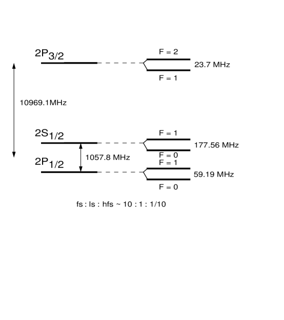
Figure 5: The experimental $n=2$ hydrogen spectrum: fine structure, Lamb shift and hyperfine structure. ${\bf F}={\bf L}+{\bf S_{e}}+{\bf S_{p}}$.

If we compare the three regions we see the following results (we only compare for the $2S_{\frac{1}{2}}$ shift since the $2P_{\frac{1}{2}}$ shift is negligible within our errors)

$$(0\leq|{\bf k}|\leq\tilde{\lambda})~{}\delta B_{{}_{Lamb}}\sim\frac{\alpha^{3}Ryd}{3\pi}\ln\left(\frac{\tilde{\lambda}}{16.64~{}Ryd}\right)\sim 46~{}{\rm MHz}~{}(2\pi\hbar)\;,~{}~{}$$ (119)

$$(\tilde{\lambda}\leq|{\bf k}|\leq b)~{}\delta B_{{}_{Lamb}}\sim\frac{\alpha^{3}Ryd}{3\pi}\ln\left(\frac{b}{\tilde{\lambda}}\right)\sim 667~{}{\rm MHz}~{}(2\pi\hbar)\;,$$ (120)

$$(b\leq|{\bf k}|\leq m)~{}\delta B_{{}_{Lamb}}\sim\frac{\alpha^{3}Ryd}{3\pi}\ln\left(\frac{m}{b}\right)\sim 334~{}{\rm MHz}~{}(2\pi\hbar)\;,$$ (121)

where we used $\tilde{\lambda}=m\alpha\sqrt{\alpha}$ and $b=m\sqrt{\alpha}$, consistent choices used throughout this chapter. As expected on physical grounds, the dominant photon momentum that couples to hydrogen is

$$|{\bf k}|\sim 1/a_{0}\sim m\alpha\;.$$ (122)

That is, the photon wavelength that couples the strongest to the neutral hydrogen system is of order the size of the system. As seen above, the effects of photons of this momentum amount to about two-thirds of the Lamb shift, the dominant part of this experimentally observed shift.

Chapter 5 Summary and Discussion

In positronium, in a consistent set of approximations, we analytically calculated the spin splitting for the $n=1$ levels through order $\alpha^{4}$. To go beyond this, and calculate the spin splitting through order $\alpha^{5}$ for example, it is clear that the effective Hamiltonian $H_{\lambda}$ must be derived through fourth order.

Kaluza and Pirner were the first to numerically calculate the ground state spin splitting of positronium (neglecting annihilation channel contributions) through order $\alpha^{4}$ in a light-front hamiltonian approach [57], but they were forced to make ad hoc assumptions because their Hamiltonian depended on the full eigenvalue of the problem. We avoided these assumptions in our approach, and performed the calculation analytically.

The dominant part of the Lamb shift was calculated with result $1043$ MHz. This turned out to be accurate, and within a consistent set of approximations was shown to be independent of our final cutoff $\tilde{\lambda}$. It was important to establish this independence to validate the placement of our final cutoff in the range $m\alpha^{2}\ll\tilde{\lambda}\ll m\alpha$—which is necessary to obtain the result in the few-body sector alone. We did not show that the result was independent of the initial cutoff $\tilde{\Lambda}$. We fixed $\tilde{\Lambda}$ such that the photon energy in the respective loop satisfied $|{\bf k}|_{photon}\leq m$, and did not derive the $\tilde{\Lambda}$-independence of the result. To obtain more precision, the full one-loop renormalization must be performed of course. A final note on the Lamb shift calculation: Each of our five diagrams (of Figures 2 and 4) were infrared ($k^{+}_{photon}\longrightarrow 0$) divergent; however, both the sum of the two low photon-energy diagrams and the sum of the three high photon-energy diagrams were infrared finite. This is an encouraging result for future work.

We close with a discussion of rotational invariance in the context of light-front field theory, and how the results of this dissertation fit into the big picture. The transverse rotation generators are dynamic and our regulator is not rotationally symmetric, thus non-covariant counterterms will in general be required to obtain a dynamic solution which adheres to the principles of rotational invariance. An initial study [60] at the one- and two-loop level in Yukawa theory showed in perturbation theory that rotationally invariant results follow with an appropriate renormalization of the kinetic and vertex masses. We continued the study of rotational invariance in this dissertation from the perspective of the QED bound-state problem. In Chapter 3 we showed in a consistent set of approximations through order $\alpha^{4}$ in the ground state spin splitting of positronium that the result is rotationally symmetric and followed from the canonical structure of the interactions; however, this result could only be obtained after including the dynamic shifts from second order bound-state perturbation theory which necessarily included a sum over all intermediate bound and scattering Coulomb states.

As is no surprise, the generators are dynamic, and rotational invariance comes about in a dynamically complicated way even at the no-loop level for the bound-state problem—analytic understanding of this was presented in Chapter 3 and may be useful for future work.

In Chapter 4 we obtained the dominant part of the Lamb shift of hydrogen consistently through order $\alpha^{5}\ln(1/\alpha)$. This showed that the level classification—$2S_{1/2}$ and $2P_{1/2}$ for this example—as dictated by rotational invariance was maintained in this example. This calculation necessarily included one-loop electron kinetic mass renormalization which followed from coupling coherence.

Neither example required the problematic diagrams mentioned in [60] with an instantaneous fermion line immediately preceding external self-energy shifts, thus we could set the vertex mass to the kinetic mass (actually it was required to get correct results). However, since the transverse rotation generators are dynamic, more nonperturbative analysis (for the positronium example) was required than in an equal-time calculation. Analytic understanding of the bound-state problem in QED in a light-front hamiltonian approach has been advanced.

Chapter 6 Summary of light-front conventions

In this appendix we write our light-front conventions for the electron, proton, and photon system (including the antiparticles). The reader unaccustomed to light-front coordinates may want to read Chapter 1 before consulting this appendix. Our conventions are

$$\bullet V^{\pm}=V^{0}\pm V^{3}~{}~{}\rm{where}~{}V^{\mu}~{}{\rm is~{}any~{}four\!\!-\!\!vector,}$$

$$\bullet \gamma^{+}=\left[\begin{array}[]{cc}0&0\\ 2i&0\end{array}\right]~{};~{}\gamma^{-}=\left[\begin{array}[]{cc}0&-2i\\ 0&0\end{array}\right]\;,$$

$$\bullet \alpha^{i}=\gamma^{0}\gamma^{i}=\left[\begin{array}[]{cc}0&\sigma^{i}\\ \sigma^{i}&0\end{array}\right]~{};~{}i=1,2~{};~{}\sigma^{i}~{}{\rm are}~{}SU(2)~{}{\rm Pauli}~{}{\rm matrices\;,}$$

$$\bullet \Lambda_{+}=\frac{1}{2}\gamma^{0}\gamma^{+}=\left[\begin{array}[]{cc}1&0\\ 0&0\end{array}\right]~{};~{}\Lambda_{-}=\frac{1}{2}\gamma^{0}\gamma^{-}=\left[\begin{array}[]{cc}0&0\\ 0&1\end{array}\right]\;,$$

$$\bullet \psi_{\pm}=\Lambda_{\pm}\psi~{};~{}\psi=\psi_{+}+\psi_{-}\;,$$

$$\bullet \psi_{e+}=\left[\begin{array}[]{c}\xi_{e}\\ 0\end{array}\right]~{};~{}\psi_{p+}=\left[\begin{array}[]{c}\xi_{p}\\ 0\end{array}\right]~{};~{}e~{}{\rm for~{}electron},~{}p~{}{\rm for~{}proton\;,}$$

$$\bullet \psi_{e-}=\left[\begin{array}[]{c}0\\ \frac{1}{i\partial^{+}}\left\{\left[\sigma^{i}\left(i\partial^{i}+eA^{i}\right)+im\right]\xi_{e}\right\}\end{array}\right]\;,$$

$$\bullet \psi_{p-}=\left[\begin{array}[]{c}0\\ \frac{1}{i\partial^{+}}\left\{\left[\sigma^{i}\left(i\partial^{i}-eA^{i}\right)+im_{p}\right]\xi_{p}\right\}\end{array}\right]\;,$$

$$\bullet A^{-}=\frac{-2}{(\partial^{+})^{2}}J^{+}+2\frac{\partial^{i}}{\partial^{+}}A^{i}\;,$$

$$\bullet J^{+}=2e\left(\xi_{p}^{\dagger}\xi_{p}-\xi_{e}^{\dagger}\xi_{e}\right)~{};~{}e>0\;,$$

$$\bullet A^{+}=0\;.$$

In momentum space the dynamical field operators are expanded as (at $x^{+}=0$)

$$A^{i}(x) = \sum_{s=\pm 1}\int_{q}(\epsilon^{i}_{s}a_{s}(q)e^{-iq\cdot x}+h.c.)\;,$$

$$\xi_{e}(x) = \sum_{s=\pm 1}\chi_{s}\int_{p}\sqrt{p^{+}}(b_{s}(p)e^{-ip\cdot x}+d_{{\overline{s}}}^{\dagger}(p)e^{+ip\cdot x})\;,$$

$$\xi_{p}(x) = \sum_{s=\pm 1}\chi_{s}\int_{p}\sqrt{p^{+}}(B_{s}(p)e^{-ip\cdot x}+D_{{\overline{s}}}^{\dagger}(p)e^{+ip\cdot x})\;,$$

$${\rm with} \epsilon_{1}^{i}=\frac{-1}{\sqrt{2}}\left(\delta_{i,1}+i~{}\delta_{i,2}\right)\;,\;\epsilon_{-1}^{i}=\frac{1}{\sqrt{2}}\left(\delta_{i,1}-i~{}\delta_{i,2}\right)\;,$$

$$\chi_{{}_{1}}=\left(\begin{array}[]{c}1\\ 0\end{array}\right)\;,\;\chi_{{}_{\overline{1}}}=\left(\begin{array}[]{c}0\\ 1\end{array}\right)\;.$$

Note that ${\overline{s}}\equiv-s$. Also, we are using the shorthand

$$\int_{p}f(p) = \int\frac{d^{4}p}{(2\pi)^{4}}~{}2\pi~{}\delta(p^{2}-m^{2})~{}\theta(p^{0})~{}f(p)=\int\frac{d^{2}p^{\perp}dp^{+}\theta(p^{+})}{16\pi^{3}p^{+}}f(p){\Biggr{|}}_{p^{-}=\frac{{p^{\perp}}^{2}+m^{2}}{p^{+}}}~{}.$$

The fermion helicity can only take on the values $\pm 1/2$, however we define $h_{3}=s/2$; therefore, “s” can only take on the values $\pm 1$. The non-vanishing commutation (anti-commutation) relations and the free Fock states are given by

$$[a_{\lambda}(q),a_{\lambda^{\prime}}^{\dagger}(q^{\prime})]=16\pi^{3}q^{+}\delta^{3}(q-q^{\prime})\delta_{\lambda\lambda^{\prime}}\;,\;[\;\delta^{3}(p)=\delta^{2}(p^{\perp})\delta(p^{+})\;]\;,$$

$$\{b_{s}(p),b_{s^{\prime}}^{\dagger}(p^{\prime})\}=\{d_{s}(p),d_{s^{\prime}}^{\dagger}(p^{\prime})\}=16\pi^{3}p^{+}\delta^{3}(p-p^{\prime})\delta_{ss^{\prime}}\;,$$

$$\{B_{s}(p),B_{s^{\prime}}^{\dagger}(p^{\prime})\}=\{D_{s}(p),D_{s^{\prime}}^{\dagger}(p^{\prime})\}=16\pi^{3}p^{+}\delta^{3}(p-p^{\prime})\delta_{ss^{\prime}}\;,$$

$$\langle p_{1}s_{1}|p_{2}s_{2}\rangle=16\pi^{3}p_{1}^{+}\delta^{3}(p_{1}-p_{2})\delta_{s_{1}s_{2}}\;,\;|p_{1}s_{1}\rangle=b_{s_{1}}^{\dagger}(p_{1})|0\rangle\;,\;{\rm etc}\;.$$

Chapter 7 Matrix elements of the canonical Hamiltonian used in the dissertation

In this appendix, the matrix elements of the canonical Hamiltonian $H$ in the basis of the free Hamiltonian $h$ that were used to derive the results in this dissertation are given. See Eqs. (49)–(57) for the operator form of $H$. These matrix elements were worked out by Allen [19]. Note that these matrix elements correspond to normal-ordered interactions with zero modes dropped.

First, some comments and notation for clarity and completeness of this appendix: $H=h+v$ where $h$ is the free field theoretic Hamiltonian. $h|i\rangle=\varepsilon_{i}|i\rangle$ and the matrix elements below are in this basis $\{|i\rangle\}$. ($e$, $p$, ${\overline{e}}$, $\gamma$) labels represent (electron, proton, positron, photon) respectively. Transverse momenta are written as $p^{i}_{1},\,p^{i}_{2},\,\ldots$ ($i=1,\,2$ only as always) and longitudinal momenta are written as $p^{+}_{1},\,p^{+}_{2},\,\ldots$. Repeated transverse indices are to be summed. The $1/2$ is factored out of the fermion helicities so all helicities below are written as $s_{1},\,s_{2},\,\ldots$, where $s_{i}=\pm 1$ only. Also note ${\overline{s}}_{i}=-s_{i}$. $m$ is the renormalized electron mass, $m_{p}$ is the renormalized proton mass and $-e$ [$e$] is the renormalized electric coupling of the electron [proton] ($e>0$). The photon polarization vectors are

$$\epsilon_{1}^{j}=\frac{-1}{\sqrt{2}}\left(\delta_{j,1}+i~{}\delta_{j,2}\right)\;,\;\epsilon_{-1}^{j}=\frac{1}{\sqrt{2}}\left(\delta_{j,1}-i~{}\delta_{j,2}\right)\;.$$ (1)

We also use

$$p^{j}(s) = p^{j}+i~{}s~{}\epsilon_{jk}~{}p^{k}\;,$$ (2)

with $\epsilon_{12}=-\epsilon_{21}=1$ and $\epsilon_{11}=\epsilon_{22}=0$. A final convenient notation is

$$\left\langle a\left|v\right|b\right\rangle=16\pi^{3}\delta^{3}(p_{a}-p_{b})\left(a|v|b\right)\;,$$ (3)

where $p_{a}$ and $p_{b}$ are total three-momenta of the respective state and $\delta^{3}(p)=\delta^{2}(p^{\perp})\delta(p^{+})$.

The eleven canonical matrix elements used in this dissertation are

$$\left(e_{2}\gamma_{3}\left|v\right|e_{1}\right) = -e\sqrt{p_{1}^{+}p_{2}^{+}}\left[\delta_{s_{1}s_{2}}\epsilon_{s_{3}}^{i\ast}\left(2\frac{p_{3}^{i}}{p_{3}^{+}}-\frac{p_{1}^{i}(s_{1})}{p_{1}^{+}}-\frac{p_{2}^{i\ast}(s_{2})}{p_{2}^{+}}\right)\right.$$ (4)

$$\hskip 61.42993pt+\left.\delta_{{\overline{s}}_{1}s_{2}}\delta_{s_{1}s_{3}}\frac{2i}{\sqrt{2}}{\overline{s}}_{1}m\left(\frac{1}{p_{2}^{+}}-\frac{1}{p_{1}^{+}}\right)\right]\;,$$

$$\left(p_{2}\gamma_{3}\left|v\right|p_{1}\right) = e\sqrt{p_{1}^{+}p_{2}^{+}}\left[\delta_{s_{1}s_{2}}\epsilon_{s_{3}}^{i\ast}\left(2\frac{p_{3}^{i}}{p_{3}^{+}}-\frac{p_{1}^{i}(s_{1})}{p_{1}^{+}}-\frac{p_{2}^{i\ast}(s_{2})}{p_{2}^{+}}\right)\right.$$ (5)

$$\hskip 61.42993pt+\left.\delta_{{\overline{s}}_{1}s_{2}}\delta_{s_{1}s_{3}}\frac{2i}{\sqrt{2}}{\overline{s}}_{1}m_{p}\left(\frac{1}{p_{2}^{+}}-\frac{1}{p_{1}^{+}}\right)\right]\;,$$

$$\left({\overline{e}}_{2}\gamma_{3}\left|v\right|{\overline{e}}_{1}\right) = e\sqrt{p_{1}^{+}p_{2}^{+}}\left[\delta_{s_{1}s_{2}}\epsilon_{s_{3}}^{i\ast}\left(2\frac{p_{3}^{i}}{p_{3}^{+}}-\frac{p_{1}^{i}(s_{1})}{p_{1}^{+}}-\frac{p_{2}^{i\ast}(s_{2})}{p_{2}^{+}}\right)\right.$$ (6)

$$\hskip 61.42993pt+\left.\delta_{{\overline{s}}_{1}s_{2}}\delta_{s_{1}s_{3}}\frac{2i}{\sqrt{2}}{\overline{s}}_{1}m\left(\frac{1}{p_{2}^{+}}-\frac{1}{p_{1}^{+}}\right)\right]\;,$$

$$\left(e_{3}\left|v\right|e_{1}\gamma_{2}\right) = -e\sqrt{p_{1}^{+}p_{3}^{+}}\left[\delta_{s_{1}s_{3}}\epsilon_{s_{2}}^{i}\left(2\frac{p_{2}^{i}}{p_{2}^{+}}-\frac{p_{1}^{i}(s_{1})}{p_{1}^{+}}-\frac{p_{3}^{i\ast}(s_{3})}{p_{3}^{+}}\right)\right.$$ (7)

$$\hskip 61.42993pt+\left.\delta_{{\overline{s}}_{1}s_{3}}\delta_{{\overline{s}}_{1}s_{2}}\frac{2i}{\sqrt{2}}s_{1}m\left(\frac{1}{p_{3}^{+}}-\frac{1}{p_{1}^{+}}\right)\right]\;,$$

$$\left(p_{3}\left|v\right|p_{1}\gamma_{2}\right) = e\sqrt{p_{1}^{+}p_{3}^{+}}\left[\delta_{s_{1}s_{3}}\epsilon_{s_{2}}^{i}\left(2\frac{p_{2}^{i}}{p_{2}^{+}}-\frac{p_{1}^{i}(s_{1})}{p_{1}^{+}}-\frac{p_{3}^{i\ast}(s_{3})}{p_{3}^{+}}\right)\right.$$ (8)

$$\hskip 61.42993pt+\left.\delta_{{\overline{s}}_{1}s_{3}}\delta_{{\overline{s}}_{1}s_{2}}\frac{2i}{\sqrt{2}}s_{1}m_{p}\left(\frac{1}{p_{3}^{+}}-\frac{1}{p_{1}^{+}}\right)\right]\;,$$

$$\left({\overline{e}}_{3}\left|v\right|{\overline{e}}_{1}\gamma_{2}\right) = e\sqrt{p_{1}^{+}p_{3}^{+}}\left[\delta_{s_{1}s_{3}}\epsilon_{s_{2}}^{i}\left(2\frac{p_{2}^{i}}{p_{2}^{+}}-\frac{p_{1}^{i}(s_{1})}{p_{1}^{+}}-\frac{p_{3}^{i\ast}(s_{3})}{p_{3}^{+}}\right)\right.$$ (9)

$$\hskip 61.42993pt+\left.\delta_{{\overline{s}}_{1}s_{3}}\delta_{{\overline{s}}_{1}s_{2}}\frac{2i}{\sqrt{2}}s_{1}m\left(\frac{1}{p_{3}^{+}}-\frac{1}{p_{1}^{+}}\right)\right]\;,$$

$$\left(\gamma_{3}\left|v\right|e_{1}{\overline{e}}_{2}\right) = -e\sqrt{p_{1}^{+}p_{2}^{+}}\left[\delta_{s_{1}{\overline{s}}_{2}}\epsilon_{s_{3}}^{i\ast}\left(2\frac{p_{3}^{i}}{p_{3}^{+}}-\frac{p_{1}^{i}(s_{1})}{p_{1}^{+}}-\frac{p_{2}^{i}(s_{2})}{p_{2}^{+}}\right)\right.$$ (10)

$$\hskip 61.42993pt+\left.\delta_{s_{1}s_{2}}\delta_{s_{1}s_{3}}\frac{2i}{\sqrt{2}}s_{1}m\left(\frac{1}{p_{1}^{+}}+\frac{1}{p_{2}^{+}}\right)\right]\;,$$

$$\left(e_{2}{\overline{e}}_{3}\left|v\right|\gamma_{1}\right) = -e\sqrt{p_{2}^{+}p_{3}^{+}}\left[\delta_{{\overline{s}}_{2}s_{3}}\epsilon_{s_{1}}^{i}\left(2\frac{p_{1}^{i}}{p_{1}^{+}}-\frac{p_{3}^{i\ast}(s_{3})}{p_{3}^{+}}-\frac{p_{2}^{i\ast}(s_{2})}{p_{2}^{+}}\right)\right.$$ (11)

$$\hskip 61.42993pt+\left.\delta_{s_{2}s_{3}}\delta_{s_{1}s_{3}}\frac{2i}{\sqrt{2}}{\overline{s}}_{3}m\left(\frac{1}{p_{2}^{+}}+\frac{1}{p_{3}^{+}}\right)\right]\;,$$

$$\left(e_{3}p_{4}\left|v\right|e_{1}p_{2}\right) = -4e^{2}\frac{\sqrt{p_{1}^{+}p_{2}^{+}p_{3}^{+}p_{4}^{+}}}{\left(p_{1}^{+}-p_{3}^{+}\right)^{2}}\delta_{s_{1}s_{3}}\delta_{s_{2}s_{4}}\;,$$ (12)

$$\left(e_{3}{\overline{e}}_{4}\left|v\right|e_{1}{\overline{e}}_{2}\right)_{exchange} = -4e^{2}\frac{\sqrt{p_{1}^{+}p_{2}^{+}p_{3}^{+}p_{4}^{+}}}{\left(p_{1}^{+}-p_{3}^{+}\right)^{2}}\delta_{s_{1}s_{3}}\delta_{s_{2}s_{4}}\;,$$ (13)

$$\left(e_{3}{\overline{e}}_{4}\left|v\right|e_{1}{\overline{e}}_{2}\right)_{annihil} = 4e^{2}\frac{\sqrt{p_{1}^{+}p_{2}^{+}p_{3}^{+}p_{4}^{+}}}{\left(p_{1}^{+}+p_{2}^{+}\right)^{2}}\delta_{s_{1}{\overline{s}}_{2}}\delta_{s_{3}{\overline{s}}_{4}}\;,$$ (14)

where these last two add as $\left(e_{3}{\overline{e}}_{4}\left|v\right|e_{1}{\overline{e}}_{2}\right)=\left(e_{3}{\overline{e}}_{4}\left|v\right|e_{1}{\overline{e}}_{2}\right)_{exchange}+\left(e_{3}{\overline{e}}_{4}\left|v\right|e_{1}{\overline{e}}_{2}\right)_{annihil}$.

Chapter 8 4th order Bloch and 3rd order G-W

In this appendix we record the fourth order effective Bloch interactions as promised in Eq. (73) of Chapter 2. Also we record the third order effective G-W interactions as promised at the end of Section 2.

First, fourth order Bloch:

$$\langle a|v_{\lambda}^{{}^{(4)}}|b\rangle = \frac{1}{2}\sum_{i,j,k}\langle a|v_{\Lambda}|i\rangle\langle i|v_{\Lambda}|j\rangle\langle j|v_{\Lambda}|k\rangle\langle k|v_{\Lambda}|b\rangle\left[\frac{1}{\Delta_{ai}\Delta_{aj}\Delta_{ak}}+\frac{1}{\Delta_{bi}\Delta_{bj}\Delta_{bk}}\right]$$ (1)

$$-\frac{1}{2}\sum_{i,c,j}\langle a|v_{\Lambda}|i\rangle\langle i|v_{\Lambda}|c\rangle\langle c|v_{\Lambda}|j\rangle\langle j|v_{\Lambda}|b\rangle\left[\frac{1}{\Delta_{ai}\Delta_{aj}\Delta_{cj}}+\frac{1}{\Delta_{bi}\Delta_{bj}\Delta_{ci}}\right.$$

$$\left.\hskip 36.135pt+\frac{1}{4}\left\{\frac{1}{\Delta_{ai}\Delta_{ci}\Delta_{cj}}+\frac{1}{\Delta_{ci}\Delta_{cj}\Delta_{bj}}-\frac{1}{\Delta_{ai}\Delta_{ci}\Delta_{bj}}-\frac{1}{\Delta_{ai}\Delta_{cj}\Delta_{bj}}\right\}\right]$$

$$-\frac{1}{2}\sum_{i,j,c}\langle a|v_{\Lambda}|i\rangle\langle i|v_{\Lambda}|j\rangle\langle j|v_{\Lambda}|c\rangle\langle c|v_{\Lambda}|b\rangle\left[\frac{1}{\Delta_{bi}\Delta_{cj}}\left\{\frac{1}{\Delta_{ci}}+\frac{1}{\Delta_{bj}}\right\}\right]$$

$$-\frac{1}{2}\sum_{c,i,j}\langle a|v_{\Lambda}|c\rangle\langle c|v_{\Lambda}|i\rangle\langle i|v_{\Lambda}|j\rangle\langle j|v_{\Lambda}|b\rangle\left[\frac{1}{\Delta_{ci}\Delta_{bj}}\left\{\frac{2}{\Delta_{ai}}+\frac{2}{\Delta_{bi}}\right\}\right.$$

$$\left.\hskip 209.58255pt+\frac{1}{\Delta_{ci}\Delta_{aj}}\left\{\frac{1}{\Delta_{ai}}+\frac{1}{\Delta_{cj}}\right\}\right]$$

$$+\frac{1}{2}\sum_{i,c,d}\frac{\langle a|v_{\Lambda}|i\rangle\langle i|v_{\Lambda}|c\rangle\langle c|v_{\Lambda}|d\rangle\langle d|v_{\Lambda}|b\rangle}{\Delta_{bi}\Delta_{ci}\Delta_{di}}$$

$$+\frac{1}{2}\sum_{c,d,i}\frac{\langle a|v_{\Lambda}|c\rangle\langle c|v_{\Lambda}|d\rangle\langle d|v_{\Lambda}|i\rangle\langle i|v_{\Lambda}|b\rangle}{\Delta_{ai}\Delta_{ci}\Delta_{di}}\;.$$

And now we record third order G-W:

$${\overline{v}}_{\lambda ij}^{{}^{(3)}} = \sum_{ab}\left[{\overline{v}}_{\Lambda ia}{\overline{v}}_{\Lambda ab}{\overline{v}}_{\Lambda bj}\left\{\frac{\xi_{1}}{\Delta_{ja}\Delta_{ab}}+\frac{\xi_{2}}{\Delta_{ja}\Delta_{jb}}\right.\right.$$ (2)

$$\left.\left.~{}~{}~{}~{}~{}~{}~{}~{}~{}~{}+\frac{\xi_{3}}{\Delta_{jb}\Delta_{ia}}+\frac{\xi_{4}}{\Delta_{jb}\Delta_{ba}}\right\}+(i\longleftrightarrow j)^{\dagger}\right]\;,$$

where

$$\xi_{1}={\overline{f}}_{\lambda ab}f_{\Lambda ab}\Theta_{bai}\Theta_{abj}\Theta_{jab}+{\overline{f}}_{\lambda aj}f_{\Lambda aj}\Theta_{jai}\Theta_{abj}f_{\Lambda ab}\Theta_{baj}\;,$$

$$\xi_{2}={\overline{f}}_{\lambda jb}f_{\Lambda jb}\Theta_{jbia}\Theta_{jba}\Theta_{ajb}+{\overline{f}}_{\lambda aj}f_{\Lambda aj}\Theta_{jai}\Theta_{jba}f_{\Lambda jb}\Theta_{bja}\;,$$

$$\xi_{3}={\overline{f}}_{\lambda bj}f_{\Lambda bj}\Theta_{jbi}\Theta_{iabj}f_{\Lambda ia}\Theta_{iab}\;,$$

$$\xi_{4}={\overline{f}}_{\lambda bj}f_{\Lambda bj}\Theta_{jbi}\Theta_{abj}f_{\Lambda ab}\Theta_{bai}\;.$$

This is for $f_{\lambda ij}=\theta(\lambda-|\Delta_{ij}|)$. Recall $f_{\lambda}+{\overline{f}}_{\lambda}=1$ and $\Delta_{ij}=\varepsilon_{i}-\varepsilon_{j}$. Note that the labels ‘$i,~{}j,~{}\ldots$’ and ‘$a,~{}b,~{}\ldots$’ span the whole energy space [unlike the notation used for Bloch; see below Eq. (73) for the notation in this case]. $\Theta_{abcd}=\theta(|\Delta_{ab}|-|\Delta_{cd}|)$ and $\Theta_{abc}=\theta(|\Delta_{ab}|-|\Delta_{bc}|)$. Note that ‘$(i\longleftrightarrow j)^{\dagger}$’ implies ‘${\overline{v}}_{\Lambda ia}{\overline{v}}_{\Lambda ab}{\overline{v}}_{\Lambda bj}\longrightarrow{\overline{v}}_{\Lambda ib}{\overline{v}}_{\Lambda ba}{\overline{v}}_{\Lambda aj}$ and $(i\longleftrightarrow j)$ in the remaining pieces of the respective term’. As advertised we see that the denominators are constrained to be between $\lambda$ and $\Lambda$ ($\lambda<\Lambda$): there are no small energy denominators (as long as $\lambda$ is not too small).

Chapter 9 Hyperspherical harmonics and Fock coordinate change

In this appendix we list some useful mathematical relations used in Chapter 3. The conventions followed here are the same as in Ref. [61]. These hyperspherical harmonics are given by

$$Y_{\nu}(\Omega) \equiv Y_{n,l,m}(\Omega)\equiv f_{n,l}(\omega)Y_{l,m}(\theta,\phi)\;,$$ (1)

where

$$0 \leq |m|\leq l\leq n-1\;.$$ (2)

These function labels $\nu=(n,\,l,\,m)$ correspond with the standard nonrelativistic quantum numbers of hydrogen. These spherical harmonics, $Y_{l,m}(\theta,\phi)$, are given by [62]

$$Y_{l,m}(\theta,\phi) = \sqrt{\frac{2l+1}{4\pi}\frac{(l-m)!}{(l+m)!}}\frac{(-1)^{m}}{2^{l}l!}(1-x^{2})^{\frac{m}{2}}\frac{d^{l+m}}{dx^{l+m}}(x^{2}-1)^{l}e^{im\phi}\;,$$ (3)

where $x=\cos\theta$. These other functions, $f_{n,l}(\omega)$, are given by

$$f_{n,l}(\omega) = (-i)^{l}\sqrt{\frac{2n(n-l-1)!}{\pi(n+l)!}}\sin^{l}\omega\frac{d^{l}}{(d\cos\omega)^{l}}C_{n-1}(\cos\omega)\;,$$ (4)

where $C_{n-1}(\cos\omega)$ are Gegenbauer polynomials. The first few are [63]

$$C_{0}(y) = 1\;,\;C_{1}(y)=2y\;,\;C_{2}(y)=4y^{2}-1\;,\;C_{3}(y)=8y^{3}-4y~{},$$

$$C_{4}(y) = 16y^{4}-12y^{2}+1\;,\;C_{5}(y)=32y^{5}-32y^{3}+6y\;.$$ (5)

The phase and orthonormality relations of these above functions are

$$Y_{n,l,m}=(-1)^{l+m}Y_{n,l,-m}^{\ast}\;,\;Y_{l,m}=(-1)^{m}Y_{l,-m}^{\ast}\;,\;f_{n,l}=(-1)^{l}f_{n,l}^{\ast}$$ (6)

and

$$\int d\Omega^{{}^{(3)}}Y_{l,m}^{\ast}Y_{l^{\prime},m^{\prime}}=\delta_{ll^{\prime}}\delta_{mm^{\prime}}\;,\;\int d\omega\sin^{2}\omega f_{n,l}^{\ast}f_{n^{\prime},l}=\delta_{nn^{\prime}}$$

$$\hskip 36.135pt\Longrightarrow\int d\Omega Y_{\nu}^{\ast}Y_{\nu^{\prime}}=\delta_{\nu\nu^{\prime}}\;,$$ (7)

where $d\Omega\equiv d\Omega^{{}^{(4)}}\equiv d\Omega^{{}^{(3)}}d\omega\sin^{2}\omega$, $0\leq\omega\leq\pi$, $0\leq\theta\leq\pi$ and $0\leq\phi\leq 2\pi$. Combining the spherical harmonics and respective derivative of the Gegenbauer polynomials, for the first few hyperspherical harmonics gives

$$Y_{1,0,0} = \frac{1}{\sqrt{2\pi^{2}}}~{}~{},~{}~{}Y_{2,0,0}=\frac{\sqrt{2}\cos\omega}{\pi}$$

$$Y_{2,1,-1} = \frac{-ie^{-i\phi}\sin\omega\sin\theta}{\pi}~{}~{},~{}~{}Y_{2,1,0}=\frac{-i\sqrt{2}\sin\omega\cos\theta}{\pi}$$

$$Y_{2,1,1} = \frac{ie^{i\phi}\sin\omega\sin\theta}{\pi}\;.$$ (8)

For further harmonics we refer the interested reader to Appendix 2 of Judd’s text [64], where this is done quite nicely.

For the coordinate change in the Coulomb Schrödinger equation of positronium [see Eq. (39) and the discussion that follows it], for ${\cal B}_{{}_{N}}<0$, we define

$$m{\cal B}_{{}_{N}} \equiv -{e_{n}}^{2}~{},$$ (9)

$$u \equiv (u_{0},{\bf u})~{},$$ (10)

$$u_{0} \equiv \cos(\omega)\equiv\frac{e_{n}^{2}-{\bf p}^{2}}{e_{n}^{2}+{\bf p}^{2}}~{},$$ (11)

$${\bf u} \equiv \frac{{\bf p}}{|{\bf p}|}\sin(\omega)\equiv\sin(\omega)\left[\sin(\theta)\cos(\phi),sin(\theta)\sin(\phi),\cos(\theta)\right]$$ (12)

$$\equiv \frac{2e_{n}{\bf p}}{e_{n}^{2}+{\bf p}^{2}}\;.$$

Note that $u_{0}^{2}+{\bf u}^{2}=1$. Conversely this coordinate change gives

$${\bf p} = \frac{e_{n}}{1+u_{0}}{\bf u}~{},$$ (13)

$$e_{n}^{2}+{\bf p}^{2} = \frac{2e_{n}^{2}}{1+u_{0}}\;.$$ (14)

We also have

$$d\Omega_{p}=\sin^{2}\omega d\omega d\Omega_{p}^{{}^{(3)}}=\left(\frac{2e_{n}}{e_{n}^{2}+{\bf p}^{2}}\right)^{3}d^{3}p~{},$$ (15)

$$\delta^{3}(p-p^{\prime})=\frac{(2e_{n})^{3}}{(e_{n}^{2}+{\bf p}^{2})^{3}}\delta(\Omega_{p}-\Omega_{p^{\prime}})=\frac{(1+u_{o})^{3}}{e_{n}^{3}}\delta(\Omega_{p}-\Omega_{p^{\prime}})~{}.$$ (16)

After this coordinate change, the nonrelativistic Schrödinger equation of positronium is trivially integrable as described below Eq. (39) in Chapter 3. Here we record the result for the bound wavefunctions and eigenvalues:

$$\phi_{\nu}({\bf p})=\frac{4(e_{n})^{\frac{5}{2}}}{(e_{n}^{2}+{\bf p}^{2})^{2}}Y_{\nu}(\Omega_{p})$$ (17)

and

$${\cal B}_{{}_{n}}=-\frac{m\alpha^{2}}{4n^{2}}\Longrightarrow e_{n}=\frac{m\,\alpha}{2\,n}$$ (18)

respectively.

Finally, a most useful relation is

$$|{\bf p}-{\bf p}^{\prime}|^{2} = \frac{(e_{n}^{2}+{\bf p}^{2})(e_{n}^{2}+{{\bf p}^{\prime}}^{2})}{4e_{n}^{2}}|u-u^{\prime}|^{2}\;.$$ (19)

This is useful because we can expand $|u-u^{\prime}|^{2}$ as follows

$$\frac{1}{|u-u^{\prime}|^{2}} = \sum_{\nu}\frac{2\pi^{2}}{n}Y_{\nu}(\Omega_{p})Y_{\nu}^{\ast}(\Omega_{p^{\prime}})\;.$$ (20)

This completes the brief discussion on the hyperspherical harmonic mathematical relations used in Chapter 3; actually, as shown in Subsection 3, the $\delta M_{{}_{2}}^{2}$ calculation requires some further formulas, which are given as they are needed.

Chapter 10 $M_{{}_{N}}^{2}$ -vs- $B_{{}_{N}}$ in positronium as an illustration

In this appendix we invert the equation

$$M_{{}_{N}}^{2} \equiv (2m+B_{{}_{N}})^{2}\;,$$ (1)

and obtain the $\alpha$-expansion for the binding energy, $-B_{{}_{N}}$. In Chapter 3 we set up a procedure to calculate the mass-squared $M_{{}_{N}}^{2}$ of positronium. This gave

$$M_{{}_{N}}^{2} = {\cal M}_{N}^{2}+b_{4}m^{2}\alpha^{4}+{\cal O}\left(\alpha^{5}\right)\;,$$ (2)

with

$${\cal M}_{N}^{2} \equiv 4m^{2}+4m{\cal B}_{{}_{N}}\;.$$ (3)

For the leading-order spectrum of $H_{\lambda}$ we obtained

$${\cal B}_{{}_{N}} = -\frac{1}{4}\frac{m\alpha^{2}}{n^{2}}\;.$$ (4)

Taking a square root of $M_{{}_{N}}^{2}$ gives

$$B_{{}_{N}} = {\cal B}_{{}_{N}}+\frac{m\alpha^{4}}{2}\left(\frac{b_{4}}{2}-\frac{1}{32n^{4}}\right)+{\cal O}\left(\alpha^{5}\right)\;.$$ (5)

Recall that $\frac{m\alpha^{4}}{2}=\alpha^{2}Ryd$. Now, in this work, Eqs. (102)–(105) are the results of our calculation of the spin splittings of $M_{{}_{N}}^{2}$ in the ground state of positronium. These were derived in the form of Eq. (2) with result

$$b_{4}(triplet)-b_{4}(singlet) = \frac{7}{3}\;.$$ (6)

Given Eq. (5) this implies

$$B_{{}_{triplet}}-B_{{}_{singlet}} = \frac{7}{6}\alpha^{2}Ryd+{\cal O}\left(\alpha^{5}\right)\;.$$ (7)

This we recognize as the well known result for the positronium system. A final note is that if the physical values of the fine structure constant and Rydberg energy ($\frac{1}{137.0}$ and $13.60\,{\rm eV}$ respectively) are applied to this previous formula, the result agrees with experiment to one-half of a percent [65].

Chapter 11 Averaging over directions

We start this appendix by calculating the following Coulomb matrix element

$$I_{\perp} \equiv \int d^{3}p\int d^{3}p^{\prime}\;\phi_{\nu}^{\ast}({\bf p}^{\prime})\frac{\left({p}^{\perp}-{p}^{\prime\perp}\right)^{2}}{({\bf p}-{{\bf p}^{\prime}})^{2}}\phi_{\nu}({\bf p})\;,$$ (1)

to verify the step taken from Eq (106) to (107). It is useful to define another integral

$$I_{z} \equiv \int d^{3}p\int d^{3}p^{\prime}\;\phi_{\nu}^{\ast}({\bf p}^{\prime})\frac{\left({p}_{z}-{p}^{\prime}_{z}\right)^{2}}{({\bf p}-{{\bf p}^{\prime}})^{2}}\phi_{\nu}({\bf p})\;.$$ (2)

Now note that

$$I \equiv I_{\perp}+I_{z}=\int d^{3}p\int d^{3}p^{\prime}\;\phi_{\nu}^{\ast}({\bf p}^{\prime})\phi_{\nu}({\bf p})=\frac{(2\pi)^{3}}{\pi}\left(\frac{m\alpha}{n}\right)^{3}\delta_{l,0}\;,$$ (3)

where in this last step we recalled Eq. (109) and the fact that the wave function at the origin is real.

For $l=0$, the wave function satisfies

$$\phi_{n,0,0}({\bf p})=\phi_{n,0,0}(|{\bf p}|)\;.$$ (4)

Thus, by symmetry, for $l=0$,

$$I_{z}=\frac{1}{3}I=\frac{(2\pi)^{3}}{3\pi}\left(\frac{m\alpha}{n}\right)^{3}\;,$$ (5)

and

$$I_{\perp}=\frac{2}{3}I=\frac{2(2\pi)^{3}}{3\pi}\left(\frac{m\alpha}{n}\right)^{3}\;.$$ (6)

For $l\neq 0$, first note that $I=0$. Thus, for $l\neq 0$,

$$I_{\perp}=-I_{z}\;;$$ (7)

we will calculate $I_{z}$ below which then implies $I_{\perp}$. Next note that in position space

$$I = -2\pi^{2}\int d^{3}x~{}\phi_{\nu}^{\ast}\left({\bf x}\right)\left({{\nabla}}^{2}\frac{1}{|{\bf x}|}\right)\phi_{\nu}\left({\bf x}\right)\;,$$ (8)

using ${\vec{\nabla}}^{2}\frac{1}{|{\bf x}|}=-4\pi\delta^{3}\left({\bf x}\right)$. Thus, for $l\neq 0$, in position space

$$I_{z} = -2\pi^{2}\int d^{3}x~{}\phi_{\nu}^{\ast}\left({\bf x}\right)\left({\nabla}_{z}^{2}\frac{1}{|{\bf x}|}\right)\phi_{\nu}\left({\bf x}\right)\;.$$ (9)

Note that there is no $|{\bf x}|\rightarrow 0$ ambiguity in this previous equation because for $l\neq 0$, the wave function vanishes at the origin. Carrying out the derivative gives

$$I_{z} = -2\pi^{2}\int d^{3}x~{}\phi_{\nu}^{\ast}\left({\bf x}\right)\left(\frac{-1+3z^{2}/|{\bf x}|^{2}}{|{\bf x}|^{3}}\right)\phi_{\nu}\left({\bf x}\right)\;.$$ (10)

This matrix element was performed in the first appendix of Bethe and Salpeter’s textbook [66]. We use two of their formulas, (3.26) and (A.29). Eq. (10) integrated gives

$$I_{z} = -2\pi^{2}~{}\overline{r^{-3}}~{}c(l,m_{l})\;,$$ (11)

with

$$\overline{r^{-3}} = \frac{1}{l(l+1)(l+\frac{1}{2})}\left(\frac{m\alpha}{n}\right)^{3}\;,$$ (12)

$$c(l,m_{l}) = -1+3\left(\frac{2l^{2}+2l-1-2m_{l}^{2}}{(2l+3)(2l-1)}\right)\;.$$ (13)

Thus, recalling Eq. (7), our result for $l\neq 0$ is

$$I_{\perp} = 2\pi^{2}~{}\overline{r^{-3}}~{}c(l,m_{l})\;.$$ (14)

For $l=1$, $I_{\perp}$ is not zero, so what is going on? The answer lies in the fact that we really want to take matrix elements in the $|j,m_{j}\rangle$ basis not the $|m_{l},m_{s}\rangle$ basis, and based on rotational invariance our results are assumed to be independent of $m_{j}$. To proceed, note that we assumed $m_{s}$ is constant in our calculation of the dominant part of the Lamb shift since it is a self-energy shift. Also note that the result, Eq. (14), is even under $m_{l}\longrightarrow-m_{l}$. Below we will use these facts to show that the Clebsch-Gordan coefficients (specifically we show it for the non-trivial case—the $2P_{\frac{1}{2}}$ states) imply

$$\langle j=1/2,m_{j}|V|j=1/2,m_{j}\rangle=$$

$$\hskip 72.26999pt\frac{1}{2l+1}\frac{1}{2s+1}\sum_{m_{l}=-l}^{l}\sum_{m_{s}=-s}^{s}\langle m_{l}m_{s}|V|m_{l}m_{s}\rangle\;.$$ (15)

For now just take this result as given. Now note that $I_{\perp}$ given by Eq. (14) averaged over $m_{l}$ vanishes,

$$\frac{1}{2l+1}\sum_{m_{l}=-l}^{l}I_{\perp}=0\;,$$ (16)

where we used

$$\frac{1}{2l+1}\sum_{m_{l}=-l}^{l}m_{l}^{2}=\frac{1}{3}l(l+1)\;,$$ (17)

an obvious result after the answer is known. This result [Eq. (16)] was used in the step that led from Eq. (106) to Eq. (107) in the dissertation.

Now we show that given ‘$m_{s}={\rm constant}$’, ‘the symmetry under $m_{l}\longrightarrow-m_{l}$’ and ‘independence of $m_{j}$’ Eq. (15) follows. Using the standard Clebsch-Gordan coefficients [48], the $2P_{\frac{1}{2}}$ expectation values are

$$\left\langle\frac{1}{2}\frac{1}{2}\right|V\left|\frac{1}{2}\frac{1}{2}\right\rangle = \frac{1}{3}\left\langle 0\frac{1}{2}\right|V\left|0\frac{1}{2}\right\rangle+\frac{2}{3}\left\langle 1-\frac{1}{2}\right|V\left|1-\frac{1}{2}\right\rangle$$ (18)

$$\hskip 72.26999pt-\frac{2\sqrt{2}}{3}\Re\left\langle 0\frac{1}{2}\right|V\left|1-\frac{1}{2}\right\rangle$$

and

$$\left\langle\frac{1}{2}-\frac{1}{2}\right|V\left|\frac{1}{2}-\frac{1}{2}\right\rangle = \frac{1}{3}\left\langle 0-\frac{1}{2}\right|V\left|0-\frac{1}{2}\right\rangle+\frac{2}{3}\left\langle-1\frac{1}{2}\right|V\left|-1\frac{1}{2}\right\rangle$$ (19)

$$\hskip 72.26999pt-\frac{2\sqrt{2}}{3}\Re\left\langle 0-\frac{1}{2}\right|V\left|-1\frac{1}{2}\right\rangle\;,$$

where on the left of the equal sign the states are in the $|jm_{j}\rangle$ basis, and on the right of the equal sign the states are in the $|m_{l}m_{s}\rangle$ basis. $\Re$ implies “the real part.” Given ‘$m_{s}={\rm constant}$’ and the symmetry under $m_{l}\longrightarrow-m_{l}$ these equations become

$$\left\langle\frac{1}{2}\frac{1}{2}\right|V\left|\frac{1}{2}\frac{1}{2}\right\rangle = \frac{1}{3}\left\langle 0\frac{1}{2}\right|V\left|0\frac{1}{2}\right\rangle+\frac{1}{3}\left\langle 1-\frac{1}{2}\right|V\left|1-\frac{1}{2}\right\rangle$$ (20)

$$\hskip 72.26999pt+\frac{1}{3}\left\langle-1-\frac{1}{2}\right|V\left|-1-\frac{1}{2}\right\rangle\;,$$

$$\left\langle\frac{1}{2}-\frac{1}{2}\right|V\left|\frac{1}{2}-\frac{1}{2}\right\rangle = \frac{1}{3}\left\langle 0-\frac{1}{2}\right|V\left|0-\frac{1}{2}\right\rangle+\frac{1}{3}\left\langle-1\frac{1}{2}\right|V\left|-1\frac{1}{2}\right\rangle$$ (21)

$$\hskip 72.26999pt+\frac{1}{3}\left\langle 1\frac{1}{2}\right|V\left|1\frac{1}{2}\right\rangle\;.$$

Given $m_{j}$ independence we can take one-half of the sum of these two terms giving

$$\frac{1}{2}\left[\left\langle\frac{1}{2}\frac{1}{2}\right|V\left|\frac{1}{2}\frac{1}{2}\right\rangle+\left\langle\frac{1}{2}-\frac{1}{2}\right|V\left|\frac{1}{2}-\frac{1}{2}\right\rangle\right]=$$

$$\hskip 14.45377pt\frac{1}{2}\left[\frac{1}{3}\left\langle 0\frac{1}{2}\right|V\left|0\frac{1}{2}\right\rangle+\frac{1}{3}\left\langle 1-\frac{1}{2}\right|V\left|1-\frac{1}{2}\right\rangle+\frac{1}{3}\left\langle-1-\frac{1}{2}\right|V\left|-1-\frac{1}{2}\right\rangle\right.$$

$$\left.\hskip 36.135pt+\frac{1}{3}\left\langle 0-\frac{1}{2}\right|V\left|0-\frac{1}{2}\right\rangle+\frac{1}{3}\left\langle-1\frac{1}{2}\right|V\left|-1\frac{1}{2}\right\rangle+\frac{1}{3}\left\langle 1\frac{1}{2}\right|V\left|1\frac{1}{2}\right\rangle\right]$$ (22)

which is equivalent to Eq. (15) for the specific case of the $2P_{\frac{1}{2}}$ states, as was to be shown.

References

- [1] K. G. Wilson, T. S. Walhout, A. Harindranath, W. M. Zhang, R. J. Perry and S. D. Głazek, Phys. Rev. D 49, 6720 (1994); M. M. Brisudová and R. J. Perry, Phys. Rev. D 54, 1831 (1996); M. M. Brisudová, R. J. Perry and K. G. Wilson, Phys. Rev. Lett. 78, 1227 (1997).
- [2] B. D. Jones, R. J. Perry and S. D. Głazek, Phys. Rev. D 55, 6561 (1997).
- [3] B. D. Jones and R. J. Perry, Phys. Rev. D 55, 7715 (1997).
- [4] R. J. Perry, in Proceedings of Hadrons 94, edited by V. Herscovitz and C. Vasconcellos (World Scientific, Singapore, 1995), [hep-th/9407056].
- [5] H. A. Bethe, Phys. Rev. 72, 339 (1947).
- [6] All terms of order were first calculated by J. Pirenne, Arch. Sci. phys. nat. 29, 121, 207, 265 (1947); V. Berestetski and L. Landau, J. exp. theor. Phys. USSR. 19, 673, 1130 (1949). Some errors in these papers were corrected by R. A. Ferrel, Phys. Rev. 84, 858 (1951).
- [7] P. A. M. Dirac, Rev. Mod. Phys. 21, 392 (1949).
- [8] P. A. M. Dirac, “Lectures on Quantum Field Theory,” (Academic Press, New York, 1966).
- [9] See “Sources for Light-Front Physics,” available via anonymous ftp from ftp.physics.ohio-state.edu in the subdirectory pub/infolight in file light.tex.
- [10] A. Bassetto, G. Nardelli and R. Soldati, Yang-Mills Theories in Algebraic Non-covariant Gauges (World Scientific, Singapore, 1991); for a fairly complete list of DLCQ references see Reference [9] and S. J. Brodsky and H. C. Pauli, Light-Cone Quantization and Quantum Chromodynamics, Recent Aspects of Quantum Fields, H. Mitter and H. Gausterer, Eds., Lecture Notes in Physics, Vol. 396 (Springer-Verlag, Berlin, 1991); B. D. Keister and W. N. Polyzou, Adv. Nucl. Phys. 20, 225 (1991); S. D. Głazek, Acta Phys. Polon. B24, 1315 (1993); R. J. Perry, [4]; S. J. Brodsky, H. C. Pauli and S. S. Pinsky, Quantum Chromodynamics and Other Field Theories on the Light Cone, Submitted to Phys. Rept., [hep-ph/9705477].
- [11] W. M. Zhang, Chin. J. Phys. 32, 717 (1994), [hep-ph/9412244]; A. Harindranath, An Introduction to Light-Front Dynamics for Pedestrians, hep-ph/9612244, [Lectures given at International School on Light-Front Quantization and Non-Perturbative QCD (To be followed by the Workshop 3-14 Jun 1996), Ames, IA, 6 May - 2 Jun 1996].
- [12] J. Kogut and L. Susskind, Phys. Rep. 8, 75–172 (1973), example on p. 90.
- [13] T. Maskawa and K. Yamawaki, Prog. Theor. Phys., 56, 270 (1976); for a recent review and references see M. Burkardt, Adv. Nucl. Phys. 23, 1 (1996); for a specific QED application see A. C. Kalloniatis and D. G. Robertson, Phys. Rev. D 50, 5262 (1994).
- [14] K. G. Wilson, T. S. Walhout, A. Harindranath, W. M. Zhang, R. J. Perry and S. D. Głazek, Phys. Rev. D 49, 6720 (1994).
- [15] Reference [7] and [9]; J. B. Kogut and D. E. Soper, Phys. Rev. D 1, 2901 (1970); D. E. Soper, “Field Theories in the Infinite-Momentum Frame,” Ph. D. Dissertation, SLAC-137 [UC-34] (TH), September, 1971; S. J. Chang and R. G. Root, Phys. Rev. D 7, 1133 (1973); S. J. Chang and T. M. Yan, Phys. Rev. D 7, 1147 (1973); T. M. Yan, Phys. Rev. D 7, 1760 (1973); T. M. Yan, Phys. Rev. D 7, 1780 (1973); H. J. Melosh, Phys. Rev. D 9, 1095 (1974); V. B. Berestetskiĭ and M. V. Terent’ev, Sov. J. Nucl. Phys. 24, 547 (1976), [Yad. Fiz. 24, 1044 (1976)]; H. Leutwyler and J. Stern, Ann. Phys. 112, 94 (1978); F. Coester, Prog. Part. Nucl. Phys. 29, 1 (1992).
- [16] S. J. Chang and R. G. Root, Phys. Rev. D 7, 1133 (1973); S. J. Chang and T. M. Yan, Phys. Rev. D 7, 1147 (1973); T. M. Yan, Phys. Rev. D 7, 1760 (1973).
- [17] A. C. Kalloniatis and D. G. Robertson, Phys. Rev. D 50, 5262 (1994).
- [18] W. M. Zhang and A. Harindranath, Phys. Rev. D 48, 4881 (1993).
- [19] B. H. Allen, “Light-Front Time-Ordered Perturbation Theory Rules,” OSU technical report, 1997 (unpublished).
- [20] W. M. Zhang and A. Harindranath, Phys. Rev. D 48, 4868 (1993).
- [21] K. Harada and A. Okazaki, Phys. Rev. D 55, 6198 (1997).
- [22] S. D. Głazek and K. G. Wilson, Phys. Rev. D 48, 5863 (1993); S. D. Głazek and K. G. Wilson, Phys. Rev. D 49, 4214 (1994).
- [23] F. Wegner, Ann. Physik 3, 77 (1994).
- [24] E. L. Gubankova and F. Wegner, Exact renormalization group analysis in hamiltonian theory: I. QED Hamiltonian on the light-front, [hep-th/9702162].
- [25] C. Bloch, Nucl. Phys. 6, 329 (1958).
- [26] E. A. Ammons, Phys. Rev. D 50, 980 (1994).
- [27] E. A. Ammons, Phys. Rev. D 54, 5153 (1996).
- [28] G. Baym, Lectures on Quantum Mechanics (Addison-Wesley Pub. Co., California, 1990).
- [29] R. J. Perry, Ann. Phys. 232, 116 (1994).
- [30] R. J. Perry and K. G. Wilson, Nucl. Phys. B403, 587 (1993).
- [31] K. G. Wilson and J. B. Kogut, Phys. Rep. C 12, 75 (1974).
- [32] K. G. Wilson, Rev. Mod. Phys. 47, 773 (1975).
- [33] K. G. Wilson, Rev. Mod. Phys. 55, 583 (1983).
- [34] K. G. Wilson, Adv. Math. 16, 170 (1975).
- [35] R. Oehme and W. Zimmermann, Commun. Math. Phys. 97, 569 (1985); R. Oehme, K. Sibold and W. Zimmermann, Phys. Lett. B147, 115 (1984); W. Zimmermann, Commun. Math. Phys. 97, 211 (1985); J. Kubo, K. Sibold and W. Zimmermann, Nucl. Phys. B259, 331 (1985); R. Oehme, Prog. Theor. Phys. Supp. 86, 215 (1986); C. Lucchesi, O. Piguet and K. Sibold, Phys. Lett. B201, 241 (1988); E. Kraus, Nucl. Phys. B349, 563 (1991) and B354, 218, 245 (1991).
- [36] Reference [29], pp. 159–161.
- [37] See for example D. Mustaki, “Chiral Symmetry and the Constituent Quark Model: A Null-Plane Point of View,” Bowling Green State University report, 1994 (unpublished), [hep-ph/9404206]; Reference [14], appendices A and B; K. Itakura, “Toward a Description of Broken Phases in Light-Front Field Theories,” Ph. D. Dissertation, University of Tokyo, December, 1996; K. Itakura and S. Maedan, “Spontaneous Symmetry Breaking in Discretized Light-Cone Quantization,” Submitted to Prog. Theor. Phys., [hep-th/9703107]; M. Burkardt and H. El-Khozondar, Phys. Rev. D 55, 6514 (1997).
- [38] H. A. Bethe and E. E. Salpeter, Quantum Mechanics of One- and Two-Electron Atoms, (Plenum Publishing Corporation, New York, 1977); see p. 117 for the formula of positronium.
- [39] V. Fock, Z. Phys. 98, 145 (1935). Further references on this subject are J. Avery, Hyperspherical Harmonics: Applications in Quantum Theory (Kluwer Academic, The Netherlands, 1989); M. Sawicki, Phys. Rev. D 32, 2666 (1985).
- [40] L. Hostler, Journal Math. Phys. (N.Y.) 5, 591,1235 (1964); J. Schwinger, ibid 5, 1606 (1964).
- [41] M. M. Brisudová and R. J. Perry, Phys. Rev. D 54, 6453 (1996).
- [42] H. J. Melosh, Phys. Rev. D 9, 1095 (1974).
- [43] S. S. Schweber, QED and the Men Who Made it: Dyson, Feynman, Schwinger, and Tomonaga (Princeton University Press, New Jersey, 1994); see p. 312 for an early QED calculation of Schwinger’s in this spirit.
- [44] W. E. Lamb and R. C. Retherford, Phys. Rev. 72, 241 (1947).
- [45] J. Schwinger (Ed.), Selected Papers on Quantum Electrodynamics, (Dover, New York, 1958).
- [46] Reference [38], p. 103.
- [47] See Chapter 5 of Reference [43], in particular note the last paragraph of Section 5.8 (the theorists were not too far behind). See footnote 13 of R. P. Feynman, Phys. Rev. 76, 769 (1949); for a modern treatment that nicely resolves this low- and high-energy matching issue see Chapter 8 [in particular pp. 173–176] of J. D. Bjorken and S. D. Drell, Relativistic Quantum Mechanics, (McGraw-Hill, New York, 1964).
- [48] Review of Particle Physics, Phys. Rev. D 54, 1 (1996).
- [49] N. M. Kroll and W. E. Lamb, Phys. Rev. 75, 388 (1949).
- [50] J. B. French and V. F. Weisskopf, Phys. Rev. 75, 1240 (1949).
- [51] S. R. Lundeen and F. M. Pipkin, Phys. Rev. Lett. 46, 232 (1981) and Metrologia 22, 9 (1986).
- [52] Yu L. Sokolov and V. P. Yakovlev, Zh. Eksp. Teor. Fiz. 83, 15 (1982); V. G. Palchikov, Yu L. Sokolov, and V. P. Yakovlev, Pisma Zh. Eksp. Teor. Fiz. 38, 347 (1983) [JETP Lett. 38, 418 (1983)].
- [53] H. Grotch, Found. Phys. 24, 249 (1994).
- [54] T. Kinoshita (Ed.), Quantum Electrodynamics, (World Scientific, Singapore, 1990). S. Weinberg, The Quantum Theory of Fields I, (Cambridge University Press, New York, 1995) [see chapter 14 for a Lamb shift calculation].
- [55] Selected papers from an American perspective on the Lamb shift over the years (for a Japanese perspective see chapter 6 of [43]): H. A. Bethe, Phys. Rev. 72, 339 (1947); N. M. Kroll and W. E. Lamb, Phys. Rev. 75, 388 (1949); J. B. French and V. F. Weisskopf, Phys. Rev. 75, 1240 (1949); R. P. Feynman, Phys. Rev. 74, 1430 (1948) and corrections in ibid. 76, 769 (1949), footnote 13; J. Schwinger, Phys. Rev. 76, 790 (1949); R. Karplus, A. Klein and J. Schwinger, Phys. Rev. 86, 288 (1952); M. Baranger, H. A. Bethe and R. P. Feynman, Phys. Rev. 92, 482 (1953); G. W. Erickson and D. R. Yennie, Ann. Phys. 35, 271, 447 (1965); M. Lieber, Phys. Rev. 174, 2037 (1968); R. W. Huff, Phys. Rev. 186, 1367 (1969); T. Appelquist and S. J. Brodsky, Phys. Rev. Lett. 24, 562 (1970); G. W. Erickson, ibid 27, 780 (1971); P. J. Mohr, ibid 34, 1050 (1975); G. Bhatt and H. Grotch, Phys. Rev. A 31, 2794 (1985); G. Bhatt and H. Grotch, Phys. Rev. Lett. 58, 471 (1987); G. Bhatt and H. Grotch, Ann. Phys. 178, 1 (1987).
- [56] R. W. Huff, Phys. Rev. 186, 1367 (1969), Table II, p. 1372 (note the typo: Y 2).
- [57] M. Kaluza and H. J. Pirner, Phys. Rev. D 47, 1620 (1993).
- [58] Uwe Trittmann, “Quantum Electrodynamics at Strong Couplings,” Ph. D. Dissertation, Max-Planck-Institut für Kernphysik, January, 1997.
- [59] D. Mustaki, S. Pinsky, J. Shigemitsu and K. Wilson, Phys. Rev. D 43, 3411 (1991).
- [60] M. Burkardt and A. Langnau, Phys. Rev. D 44, 3857 (1991).
- [61] B. R. Judd, Angular Momentum Theory for Diatomic Molecules (Academic, New York, 1975), p. 32.
- [62] J. D. Jackson, Classical Electrodynamics (Wiley, New York, 1975), pp. 98–100.
- [63] Reference [61], pp. 32 and 37.
- [64] Reference [61], p. 222.
- [65] C. Itzykson and J. B. Zuber, Quantum Field Theory (McGraw-Hill, New York, 1980), p. 493.
- [66] Reference [38], pp. 17 and 348.