Effective theories for real-time correlations in hot plasmas

Abstract

We discuss the sequence of effective theories needed to understand the qualitative, and quantitative, behavior of real-time correlators $\langle{\cal A}(t){\cal A}(0)\rangle$ in ultra-relativistic plasmas. We analyze in detail the case where $\cal A$ is a gauge-invariant conserved current. This case is of interest because it includes a correlation recently measured in lattice simulations of classical, hot, SU(2)-Higgs gauge theory. We find that simple perturbation theory, free kinetic theory, linearized kinetic theory, and hydrodynamics are all needed to understand the correlation for different ranges of time. We emphasize how correlations generically have power-law decays at very large times due to non-linear couplings to long-lived hydrodynamic modes.

I Introduction

There is a rich variety of spatial and temporal scales in hot, weakly coupled, ultra-relativistic gauge theories, a selection of which are shown in Table I. Depending on the problem of interest, a wide variety of methods can be appropriate for describing the physics on different scales: naive perturbation theory, hard thermal loops, dimensional reduction, kinetic theory, Vlasov equations, Langevin equations, hydrodynamics, and more. For static properties of plasmas, the tower of effective theories relevant to different distance scales is well understood [1]. These effective theories are all Euclidean quantum field theories, in 3 or 4 dimensions, and may be systematically constructed using standard renormalization group techniques.

For real-time properties, including the analysis of non-equilibrium response, constructing an appropriate sequence of effective theories which correctly disentangles dynamics on different distance (or time) scales is much less straightforward. Some of the difficulties are illustrated by the long confusion over one of the basic time scales of hot non-Abelian plasmas: the time scale for non-perturbatively large fluctuations in gauge fields (such as those responsible for baryon number violation in electroweak theory) [2]. To elucidate the real-time dynamics of hot gauge theories, one should understand the tower of effective theories appropriate for different time scales and, at least in simple examples, calculate the appropriate matching between such theories.

typical particle wavelength	$T^{-1}$
typical particle separation	$T^{-1}$
Debye length	$(gT)^{-1}$
plasma frequency	$(gT)^{-1}$
non-perturbative magnetic length scale	$(g^{2}T)^{-1}$	(non-Abelian theories)
mean free path: any-angle scattering	$(g^{2}T\ln)^{-1}$
mean free path: large-angle scattering	$(g^{4}T\ln)^{-1}$
temporal scale for topological transitions	$(g^{4}T)^{-1}$	(non-Abelian theories)

TABLE I.: Orders of magnitude of various distance and time scales in hot, ultrarelativistic, gauge theory for weak coupling. Here, and henceforth, “$\ln$” stands for $\ln(g^{-2})$, except for the case of the mean free path for any-angle scattering in an Abelian gauge theory, where it is a genuine logarithmic infrared divergence. (Naturally, $c\equiv\hbar\equiv 1$.)

The current interest in hot electroweak baryon number violation has motivated substantial efforts in numerical simulations of hot, classical, lattice gauge theory [3, 4, 5, 6]. For certain time and distance scales, it has been argued that classical simulations can adequately reproduce the behavior of the underlying quantum plasma of interest (or more generally, that certain classical lattice results can be translated into corresponding results for the continuum quantum theory [7].) Hence, these simulations are a source of “data” for comparison with theoretical pictures of hot gauge theories. In particular, there have been recent measurements by Tang and Smit [6] of time-dependent correlations $\langle{\cal A}(t){\cal A}(0)\rangle$ for several gauge invariant operators $\cal A$. An interesting theoretical goal is then to understand how best to describe the physics of, and calculate the behavior of, such time-dependent correlators for different ranges of time.

In order to keep the discussion focussed, we shall specialize to the particular class of correlations where the operator ${\cal A}$ is the spatial part ${\bf j}$ of a conserved gauge-invariant current $j_{\mu}$ (such as the electric charge current in QED, or fermion number current in QCD). As we shall explain below, one of the correlations measured by Tang and Smit falls into this class. We shall also focus on the spatial average of such currents,

$${\cal A}(t)={\bf j}(t)\equiv V^{-1}\int d^{3}x\>{\bf j}({{\bf x}},t),$$ (1)

as did Tang and Smit. However, the principles and techniques underlying our discussion are not limited to this chosen class of examples. As our interest is in the dynamics of hot gauge theories, we shall assume that the current $j_{\mu}$ involves particles which feel a gauge force with coupling $g$. We also assume that there is no chemical potential, so that the total charge $\int d^{3}x\>j^{0}$ has zero expectation.

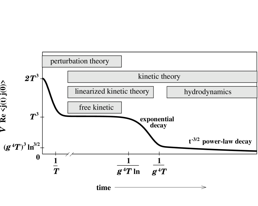
FIG. 1.: A qualitative picture of the real part of the current-current correlation $V\langle{\bf j}(t){\bf j}(0)\rangle$ in a hot plasma, for the case of bosonic charge carriers. The labels on the axes are only meant to denote orders of magnitude, except that the “$2T^{3}$” mark is in fact twice the “$T^{3}$” mark in the small-coupling limit. The time axis should be thought of as linear before the break and logarithmic after; the vertical axis should be thought of as linear. $\ln$ is short for $\ln(g^{-2})$. The transient shown at $t\sim 1/T$ decays exponentially. If the current is carried by fermions instead of scalars, the resulting graph is identical except for the initial transient, which starts from minus the “$T^{3}$” plateau value instead of twice that value.

FIG. 2.: Similar to fig. 2, but for a classical field theory defined on an infinite spatial lattice with lattice spacing $a$. We have specialized to a current ${\bf j}$ associated with a non-Abelian symmetry. The Abelian case is identical except that $g^{18}T^{11}a^{8}\ln^{5/2}$ and $\beta_{\rm L}^{-11}\ln^{5/2}$ on the left and right axes should be replaced by $g^{20}T^{12}a^{9}\ln^{2}$ and $\beta_{\rm L}^{-12}\ln^{2}$, respectively. The bottom and left axes are labeled in physical units. The top and right axis are labeled in lattice units, where the current ${\bf j}$ has been multiplied by $g^{2}$ as compared to the continuum normalization and $\beta_{\rm L}=\#(g^{2}Ta)^{-1}$. Here, $\ln$ is short for $\ln\beta_{\rm L}\sim\ln[(g^{2}Ta)^{-1}]$. The envelope of the transient oscillations decays as $t^{-5/2}$.

Fig. 2 qualitatively depicts our basic results for the time dependence of the current-current correlator, and the physical pictures best suited to understanding the dynamics at different time scales. The purpose of this paper will be to explain this graph. We have assumed that the gauge symmetry, and the symmetry corresponding to the current, are unbroken. We have also assumed that the current is normalized so that the corresponding number operator $\int d^{3}x\>j^{0}$ counts each particle as $\pm O(1)$ [rather than $\pm O(g)$, which would be conventional for the electric current]. And we assume that the underlying theory is weakly coupled: $g^{2}(T)\ll 1$.

As will be discussed later, naive perturbation theory in the underlying quantum field theory is sufficient to understand the behavior at early times. At later times, it is appropriate to treat the excitations of the theory as (quasi-)particles with definite position and momentum and to apply kinetic theory. At very late times, it is most convenient to focus on the long-wavelength, collective, hydrodynamic excitations of the system. As will be discussed below, the non-linear coupling of the current to these hydrodynamic excitations gives rise to a long-time power-law tail in the decay of the correlation function.

The behavior of the current-current correlation will turn out to be dominated by excitations of hard thermal modes—that is, modes with momentum $p$ of order $T$ in the continuum theory. As a result, some of the interesting physics of hot plasmas (such as the soft, $p\sim g^{2}T$, SU(2)-colored gauge fluctuations responsible for electroweak baryon number violation) will not be probed in our leading-order investigation, and the corresponding effective theories [2, 7, 8] do not appear in fig. 2.

Fig. 2 shows the corresponding result for a classical field theory on an infinite spatial lattice. (The finite volume case will be discussed in sec. V.) We shall later explain the causes of the qualitative differences (e.g., the short time oscillations and the different power-law decay of the long-time tail) from fig. 2. The differences between figs. 2 and 2 reflect the fact that the current-current correlator is sensitive to the hard thermal modes at all times, even in the long time limit. Such modes do not have occupation numbers large compared to one, and will never be adequately described by a classical theory. The differing origins of the long time tails in figs. 2 and 2 will be discussed in detail in section IV.

In this paper, we focus on a qualitative discussion of the correlator. A quantitative treatment of some aspects will be deferred to a companion paper [9]. Throughout this paper, orders of magnitude given for time and distance scales will refer to the case of continuum theory unless we explicitly refer to classical lattice theory. In sec. II, we examine the short-time current correlations using simple perturbation theory, and discuss the reduction to kinetic theory at times large compared to $1/T$ (continuum) or $1/a$ (classical lattice). A discussion of the leading-order perturbative result may also be found in ref. [10], which appeared as our work was being completed. In sec. III, we discuss the current correlator in the context of kinetic theory, and explain the exponential decay at intermediate times, as shown in fig. 2. Section IV reviews the existence of long-time power-law tails in systems with hydrodynamic behavior and shows how they arise in the case of the current-current correlator. In particular, we discuss the failure of classical lattice simulations to reproduce the long-time behavior of the continuum theory. Sec. V explains how the behavior of the current correlation changes qualitatively in finite volume systems. Finally, having (we hope) made clear to the reader that classical lattice simulations need not generate the same long time behavior as high temperature quantum theories, sec. VI briefly reviews the limited class of questions for which real-time classical simulations may be useful. The bulk of the paper focuses on currents in theories for which the associated charge is carried by a scalar field. (These are the theories for which it is interesting to compare the dynamics of the continuum quantum theory with the corresponding classical lattice field theory.) However, all the discussion of continuum quantum dynamics also applies to theories where fermion fields carry the global charge of interest. Appendix A discusses the small differences between results for bosonic and fermionic charge carriers.

In the remainder of this introduction, we review the correlator measured by Tang and Smit. Their interest was in electroweak theory, and they simulated SU(2) gauge theory coupled to a doublet Higgs scalar $\phi$. One of the correlations they measured was of the spatial average of the gauge-invariant operator

$${\bf W}_{a}\equiv{1\over 2i}\,{\rm tr}\left([\Phi^{\dagger}({\bf D}\Phi)-({\bf D}\Phi)^{\dagger}\Phi]\tau_{a}\right),$$ (2)

where ${\bf D}$ is the SU(2) covariant (spatial) derivative, $\tau_{a}$ is a Pauli matrix, and $\Phi$ is a $2\times 2$ matrix made up of $\phi$ and its charge conjugate:

$$\Phi=(i\tau_{2}\phi^{*},~{}\phi).$$ (3)

They chose this operator because they were interested in studying the thermal properties of gauge bosons. Well into the symmetry-broken phase of the theory, ${\bf W}_{a}$ is an operator that, to leading order, simply creates or destroys massive gauge bosons: ${\bf W}_{a}\sim\langle\phi\rangle^{2}{\bf A}_{a}$. However, ${\bf W}_{a}$ has another interpretation: it is the current associated with the global SU(2)_R custodial symmetry of the gauge-Higgs system. Specifically, the theory is invariant under the SU(2)_L$\times$SU(2)_R symmetry

$$\Phi\to L\Phi R^{\dagger},$$ (4)

where $L$ and $R$ are independent SU(2) rotations. The SU(2)_L symmetry is gauged, and the SU(2)_R symmetry is an additional global symmetry for which ${\bf W}_{a}$ is the spatial part of the current.

The SU(2)_R symmetry is broken in the low temperature phase of the theory (though the vectorial combination of SU(2)_R and SU(2)_L survives to guarantee equality of the W and Z boson masses). In this paper, we shall focus on the hot, symmetric phase of the theory. In this case, the operator ${\bf W}_{a}$ does not simply create and destroy gauge bosons, and it is more usefully thought of as a current carried by the scalars. Indeed, ${\bf W}_{a}$ cannot couple to a state composed only of gauge bosons because ${\bf W}_{a}$ carries an SU(2)_R charge [$a$ is an SU(2)_R adjoint index] while the gauge bosons do not.

II Perturbation theory

In this and the following sections, we consider Abelian or non-Abelian gauge theories with scalar and/or fermionic matter with a conserved, gauge-invariant current $j_{\mu}$. The simplest example to keep in mind is QED, coupled to either scalars or fermions, where $j_{\mu}$ is the electric current. For non-Abelian gauge theories, the gauge currents are not gauge-invariant, and we do not wish to consider unphysical objects like gauge-dependent correlators. In the non-Abelian case, we must therefore consider currents associated with additional global symmetries among the matter fields, such as the SU(2)_R custodial symmetry of the SU(2)-Higgs theory.

One way to approximate correlators is by straightforward expansion in diagrammatic perturbation theory. Fig. 3 shows the leading contribution to a current-current correlator $\langle{\bf j}(t){\bf j}(0)\rangle$. The result (for scalar fields) is

$$V\langle j_{i}(t)j_{j}(0)\rangle={\textstyle{1\over 3}}\,\delta_{ij}\,q^{2}\int_{\bf p}\>v_{\bf p}^{2}\left[\,n_{\omega_{\bf p}}e^{i\omega_{\bf p}t}+(1+n_{\omega_{\bf p}})e^{-i\omega_{\bf p}t}\,\right]^{2},$$ (5)

where $\omega_{\bf p}$ is the energy of an excitation with momentum ${\bf p}$, ${\bf v}_{\bf p}\equiv\nabla_{\bf p}\omega_{\bf p}$ is its group velocity (so $v_{\bf p}^{2}=(p/\omega_{p})^{2}$ for Lorentz invariant continuum theories), and $\int_{\bf p}$ is short for $\int d^{3}p/(2\pi)^{3}$. (See appendix A for the case of fermionic charge carriers.) $n_{\omega}$ is the Bose distribution,

$$n_{\omega}\equiv{1\over e^{\hbar\beta\omega}-1},$$ (6)

where $\hbar$ has been shown explicitly for the first and last time in this paper. The case of classical field theory may be obtained by taking the $\hbar\to 0$ limit of the Bose distribution, so that

$$1+n_{\omega}\to n_{\omega}\to{1\over\beta\omega}\,.$$ (7)

In (5), $q^{2}$ is the appropriate sum of squared charges, for the particular current under consideration, of different particle species. ($q^{2}$ is 1 for the number current of a single complex scalar. For non-Abelian currents such as (2), $q^{2}$ should be multiplied by $2\delta_{ab}$.) For convenience, we will assume throughout that the currents of interest are normalized such that $q^{2}$ is $O(1)$.

FIG. 3.: The leading-order perturbative diagram for $\langle{\bf j}(t){\bf j}(0)\rangle$.

We can split the result (5) into an asymptotic constant $q^{2}C$ and a decaying transient $q^{2}D(t)$ by rewriting it as

$$V\langle j_{i}(t)j_{j}(0)\rangle=\delta_{ij}\,q^{2}[\,C+D(t)],$$ (9)

with

$$C = {\textstyle{2\over 3}}\int_{\bf p}v_{\bf p}^{2}\;n_{\omega_{\bf p}}(1+n_{\omega_{\bf p}}),$$ (10)

$$D(t) = {\textstyle{1\over 3}}\int_{\bf p}v_{\bf p}^{2}\left[n_{\omega_{\bf p}}^{2}e^{2i\omega_{\bf p}t}+(1+n_{\omega_{\bf p}})^{2}e^{-2i\omega_{\bf p}t}\right].$$ (11)

Note that $\langle{\bf j}(t){\bf j}(0)\rangle$ is real for classical field theory but not for quantum field theory, because in the latter case ${\bf j}(t)$ and ${\bf j}(0)$ do not commute. The imaginary part only appears in the transient $q^{2}D(t)$.

The asymptotic constant $q^{2}C$ has a simple physical interpretation: Eq. (10) is precisely the result one would obtain for the expectation $\langle{\bf j}(0){\bf j}(0)\rangle$ in an ideal Bose gas of particles (and anti-particles) rather than of fields. These particles may be regarded as classical (with definite position and momentum) except that they satisfy Bose or Fermi statistics. We shall refer to this as a kinetic theory description of the plasma. The current is $q{\bf v}$ for each particle. Because velocities of particles do not change with time in an ideal gas, $\langle{\bf j}(t){\bf j}(0)\rangle=\langle{\bf j}(0){\bf j}(0)\rangle=q^{2}\langle{\bf v}(0){\bf v}(0)\rangle$ is a constant for such a gas. Note that $q^{2}C$ is real, as it should be since ${\bf j}(t)$ is real and commuting in the kinetic theory approximation.

The decaying transient $q^{2}D(t)$, on the other hand, can be seen to arise from an interference between particle and anti-particle contributions in field theory. Consider, for example, a complex scalar field $\phi$ written in terms of creation and annihilation operators:

$$\phi(x)=\int_{\bf p}{e^{i{\bf p}\cdot{\bf x}}\over\sqrt{2\omega_{\bf p}}}\left(a_{\bf p}e^{i\omega_{\bf p}t}+b_{-{\bf p}}^{\dagger}e^{-i\omega_{\bf p}t}\right),$$ (12)

where we have used non-relativistic normalization for $a_{\bf p}$ and $b_{\bf p}$. A (space-averaged) number current in a continuum scalar theory would then be

$${\bf j}(t)={-i\over V}\int_{\bf x}\phi^{\dagger}{\buildrel\leftrightarrow\over{\nabla}}\phi=\int_{\bf p}{\bf v}_{\bf p}\left[N_{\bf p}+\overline{N}_{-{\bf p}}+a_{\bf p}^{\dagger}b_{-{\bf p}}^{\dagger}e^{-2i\omega_{\bf p}t}+b_{-{\bf p}}a_{\bf p}e^{2i\omega_{\bf p}t}\right],$$ (13)

where $N_{\bf p}=a_{\bf p}^{\dagger}a_{\bf p}$ and $\overline{N}_{\bf p}=b_{\bf p}^{\dagger}b_{\bf p}$ are the number operators for particles and anti-particles, respectively (and $\int_{\bf x}$ is, of course, short for $\int d^{3}x$). Now consider the correlator $\langle{\bf j}(t){\bf j}(0)\rangle$. The non-oscillatory terms in the current (13) correspond to the kinetic theory description and are responsible for the asymptotic constant discussed before. The oscillatory pieces of the current, involving interference between particle and anti-particle contributions, are responsible for the transient behavior of the correlator. These oscillations become irrelevant at large times because contributions from different momenta ${\bf p}$ decohere.

If we treat the particles as massless, then the only frequency scale in the problem is $T$ for the continuum theory, or the cutoff $a^{-1}$ for the classical lattice theory. The time scale for the decay of the transient $D(t)$ is therefore $1/T$ or $a$, respectively, and this is the origin of the transients at those scales in figs. 2 and 2.

In the case (7) of classical field theory, for a current carried by bosons, the expression (3) for the transient contribution directly gives $D(0)=C$. Hence, in leading-order perturbation theory, the correlation decays by exactly a factor of 2 from its initial value, as shown in fig. 2. The same thing is true of the thermal contribution to the correlator in quantum field theory. The zero-temperature contribution to the correlator [$n\to 0$ in (3)], in the limit of negligible masses (so that $\omega_{p}=|{\bf p}|$), generates a $1/t^{3}$ imaginary part for the correlator.

The decay of the transient can be understood by analyzing the long-time behavior of D(t). Expressing (11) in terms of a spectral weight,

$$D(t) = {\textstyle{1\over 3}}\int_{0}^{\infty}d\omega\>\rho_{vv}(\omega)\left[n_{\omega}^{2}\,e^{2i\omega t}+(1+n_{\omega})^{2}e^{-2i\omega t}\right]$$ (14)

$$= {\textstyle{1\over 3}}\int_{-\infty}^{\infty}d\omega\>\rho_{vv}(\omega)\,n_{\omega}^{2}\,e^{2i\omega t},$$ (15)

with

$$\rho_{vv}(\omega) = \int_{\bf p}v_{\bf p}^{2}\>\delta(\omega-\omega_{\bf p}),$$ (16)

converts the problem to a standard exercise analyzing the asymptotic behavior of a Fourier transform. (In (15), we used $1+n_{\omega}=-n_{-\omega}$.) This asymptotic behavior is determined by non-analyticities of the integrand. If we ignore the mass $m$, then in the continuum case with $\omega_{p}=p$, the integrand is analytic in a strip about the real axis. Consequently, the long-time behavior decreases exponentially with an exponent determined by the imaginary part of the nearest singularity in the complex $\omega$ plane (which is at $\pm 2\pi iT$). So the decay shown in fig. 2 at $t\sim 1/T$ is exponential. In fact, in this particular case, one can find an exact analytic result for all times,

$$C={\textstyle{1\over 9}}T^{3},\qquad D(t)={{\textstyle{1\over 3}}T^{3}\over\sinh^{2}(2\pi Tt)}\left[(2\pi Tt+i\pi)\coth(2\pi Tt)-1^{\vphantom{2}}\right].$$ (17)

For a classical lattice theory, the situation is somewhat different. In this case, (7) and (10) then imply that the steady-state value $C$ is dominated by momenta of order the inverse lattice spacing $1/a$ rather than $T$, with the result that $C\sim T^{2}/a$. Also, the density $\rho_{vv}(\omega)$ (16) has kink singularities generated from points at the edge of the Brillouin zone where ${\bf v}_{\bf p}=0$. These are the well-known Van Hove singularities which appear in the electronic density of states in crystals. Such kink singularities produce an oscillating power-law tail in Fourier transforms, with the frequency of oscillations determined by the location of the singularities. This is the source of the oscillations in the $t\lesssim a$ transient shown in fig. 2. The envelope of the oscillations decays like $t^{-5/2}$; a detailed expression for the long-time behavior of $D(t)$ is given in appendix B.

Finally, let us go one step beyond the naive perturbation theory we have considered so far. It is well known that perturbation theory can be improved for high temperatures by resumming “hard thermal loops” [11]. In particular, this means including the effective thermal mass in propagators. The thermal contribution to the mass $m$ is $O(gT)$ in the continuum, and $O(g\sqrt{T/a})$ for classical lattice theories. In the presence of a mass, there will be discontinuities in $\rho_{vv}(\omega)$ at $\omega=\pm m$. These give rise to an additional power-law contribution to the long-time behavior of $D(t)$ that oscillates with frequency $m$. These oscillations have not been shown in figs. 2 and 2 because they are sub-leading compared to the total correlation: the amplitude of the transient has already decayed to $O(g)$ by the time the mass oscillations begin. See the complete expressions in appendix B for details.

III Kinetic Theory

In the last section, we saw that the leading-order perturbative result for the correlator quickly settles down to the kinetic theory result for a non-interacting gas. In the kinetic theory picture, it is easy to see that the effect of interactions will become crucial at late times, and so simple (one loop) perturbation theory must break down. Currents are produced by fluctuations in the plasma. Imagine focusing attention on some region of space (with a size large compared to the inter-particle separation). Suppose that, at time zero, a few more positive charged particles happen to be moving left rather than right and/or a few more negative charged ones are moving right rather than left, as depicted in fig. 4, so that there is a net current ${\bf j}(0)$ to the left. As time progresses, the directions of the particles will be progressively randomized by collisions, causing the net current to decay and the correlation $\langle{\bf j}(t){\bf j}(0)\rangle$ to approach zero.

FIG. 4.: A pictorial example of a typical fluctuation with net current ${\bf j}$.

A quantitative analysis of the effect of interactions will be enormously simplified if one can indeed forget about quantum field theory for times large compared to $1/a$ or $1/T$, and instead study the dynamics using kinetic theory. Kinetic theory applies to times and distances large compared to particle energies and momenta. In addition, the validity of kinetic theory requires that de Broglie wavelengths and scattering durations be small compared to the mean free path and mean free time between collisions, respectively. This ensures that particles can be viewed as propagating classically (with on-shell energies) between collisions which are independent, uncorrelated events. Whether these conditions are satisfied depends on the typical momenta and dominant scattering processes that contribute to a given physical problem. In the case at hand, it will be easiest to assume the validity of kinetic theory and return later to check the conditions.

Mean free times

To begin, it will be convenient to review some well-known basic scales associated with the times between collisions. Scattering among particles that carry gauge charges is dominated by $t$-channel exchange of a gauge boson, as depicted in fig. 5. Consider a collision between typical particles in the plasma, each with momentum of order $T$. For continuum relativistic particles, the differential cross-section is

$$n\,d\sigma\sim ng^{4}{dt_{\rm M}\over t_{\rm M}^{2}}\sim{g^{4}T}{d\theta\over\theta^{3}}$$ (18)

if we (temporarily) ignore plasma effects on the interaction. Here, $t_{\rm M}=-Q^{2}$ is the virtuality of the exchanged gauge boson, $\theta$ is the angle by which one of the particles is scattered, and we’ve multiplied $d\sigma$ by the density $n\sim T^{3}$ of scatterers. The time between single, large-angle ($\theta\sim 1$) scatterings of particles is therefore $O(1/g^{4}T)$.

FIG. 5.: t-channel gauge boson exchange. The solid lines represent any sort of particles that couple to the gauge force.

The total cross-section, however, is dominated by small-angle scatterings. Eq. (18) looks like it will lead to a linear infrared divergence in $t$, but plasma effects appear when $\sqrt{t_{\rm M}}$ is comparable to the inverse Debye screening length $\sim gT$ (corresponding to $\theta\sim g$). At this scale, Coulomb interactions are Debye screened, and magnetic interactions are suppressed by Landau damping of time-dependent, space-like magnetic fields. The damping of such magnetic fields is a reflection of the conductivity of the plasma and Lenz’s law that a conducting system resists changes in the magnetic field. If all Coulomb and magnetic interactions became completely irrelevant for $\sqrt{t_{\rm M}}\ll gT$, then the mean free time for scattering through any angle would be order $1/g^{2}T$ and dominated by $\theta\sim g$. However, the plasma does not damp static magnetic fields, and so it does not completely damp nearly-static ones. Magnetic interactions remain significant in the small region of phase space in which the energy transfer (in the plasma rest frame) of the colliding particles is very small. This phase space suppression turns out to convert the linear small-$t_{\rm M}$ divergence of (18) into a logarithmic divergence $dt_{\rm M}/t_{\rm M}$ when $\sqrt{t_{\rm M}}\lesssim gT$. In non-Abelian gauge theories, this logarithmic divergence is then cut off by non-perturbative magnetic physics at a scale of $\sqrt{t_{\rm M}}\sim g^{2}T$ ($\theta\sim g^{2}$). Hence, there is a logarithmic enhancement in the scattering rate and so a logarithmic suppression in the mean free time $\tau_{\rm small}$ for any-angle scattering:

$$\tau_{\rm small}\sim{1\over g^{2}T\ln},$$ (19)

where “$\ln$”, for non-Abelian theories, means $\ln[(gT)/(g^{2}T)]\sim\ln(g^{-1})$. The mean free time for any-angle scattering of gluons in particular is typically referred to as the plasmon damping rate (in this case, for hard gluons).

A different quantity of importance is the time it takes for the direction of a single particle to be changed by a large angle ($\theta\sim 1$). As discussed above, this can happen by a single, large-angle scattering in a time of order $1/g^{4}T$. However, it can alternatively happen by a succession of scatterings through a small angle $\Delta\theta$. The time between such scatterings is of order $(\Delta\theta)^{2}/g^{4}T$, provided that $\sqrt{t_{\rm M}}\gtrsim gT$ (or $\Delta\theta\gtrsim g$) so that there are no suppressions by the screening and damping effects discussed above. Treating successive scattering as a random walk, order $1/(\Delta\theta)^{2}$ such scatterings are needed to build up a total deviation of $\theta\sim 1$. So a succession of scatterings by $\Delta\theta$ also takes a time of order $1/g^{4}T$ to give large-angle scattering. Since all possible decades of $\Delta\theta$ contribute equally, the net result is a logarithmic enhancement in the large-angle scattering rate, $\tau_{\rm big}^{-1}\sim g^{4}T\int{d(\Delta\theta)/(\Delta\theta)}$. The mean free time $\tau_{\rm big}$ for large-angle scattering is then

$$\tau_{\rm big}\sim{1\over g^{4}T\ln}.$$ (20)

This time, the logarithm is cut off by $T$ in the ultraviolet and $gT$ in the infrared, but it’s still $\ln(g^{-1})$. The non-perturbative physics associated with the scale $g^{2}T$ in non-Abelian plasmas is not involved at leading order.

For classical lattice theories, the above analysis can be repeated, but the typical momenta of particles is $a^{-1}$ rather than $T$, the density is $n\sim Ta^{-2}$, the Debye mass scale is $\beta_{\rm L}^{-1/2}a^{-1}$, and the scale for non-perturbative magnetic physics in non-Abelian gauge theory is $\beta_{\rm L}^{-1}a^{-1}$, where the lattice coupling $\beta_{\rm L}^{-1}$ is order $g^{2}Ta$ in physical units. This results in $\tau_{\rm big}\sim\beta_{\rm L}^{-2}a/\ln(\beta_{\rm L})\sim[g^{4}T^{2}a\ln(\beta_{\rm L})]^{-1}$ for the large-angle scattering time and $\tau_{\rm small}\sim\beta_{L}^{-1}a/\ln\sim(g^{2}T^{2}a\ln)^{-1}$ for the any-angle scattering time, where “$\ln$” is $\ln(\beta_{\rm L})$ in non-Abelian gauge theory.

The correlator

So which scattering time controls the decay of the $\langle{\bf j}(t){\bf j}(0)\rangle$ correlator? Return to the picture of a typical fluctuation at time zero that has a net current ${\bf j}(0)$, illustrated in fig. 4. The total current ${\bf j}=\sum_{s}{\bf j}^{(s)}$ is the sum of currents ${\bf j}^{(s)}=q^{(s)}{\bf v}^{(s)}$ of the individual particles (labeled by $s$). Any one of those individual currents will only change substantially when the velocity ${\bf v}^{(s)}$ changes substantially. That means the relevant time scale for the randomization of the current is the mean free time $\tau_{\rm big}$ for large-angle scattering, rather than the mean free time $\tau_{\rm small}$ for any-angle scattering. This is the physics responsible for the period of exponential decay starting at time $1/(g^{4}T\ln)$ in fig. 2 [and time $1/(g^{4}T^{2}a\ln)$ in fig. 2].

There has been confusion in the literature on the above point. In ref. [10], for example, it was suggested that the way to understand the decay of the correlators measured by Tang and Smit is simply to include thermal widths (the imaginary part of the self-energy) in the internal propagators of the leading-order perturbative diagram, fig. 3. The imaginary part of the self-energy measures the rate for a particle to scatter into any other state and so includes very small-angle scatterings—that is, the width is of order $\tau_{\rm small}^{-1}$. The inclusion of widths in the diagram of fig. 3 makes the internal propagators decay on a time scale of $\tau_{\rm small}$ and therefore appears to predict that the correlation decays on a time scale of $\tau_{\rm small}$ instead of $\tau_{\rm big}$. The problem with this reasoning becomes apparent if one realizes that it could be applied to any correlator at all, including the total charge correlator $\langle j^{0}(t)j^{0}(0)\rangle$ (where $j^{0}(t)\equiv\int_{\bf x}j^{0}({\bf x},t)$). By conservation of charge, the latter does not decay at all with time. The problem is that the decay seemingly generated by resumming self-energies into fig. 3 is canceled by other, higher-order diagrams in the resummed perturbation theory. An explicit example of such cancelations for QED plasmas can be found in ref. [14]. This highlights the dangers of using resummed perturbation theory for intuition about physics at large times. A (highly non-trivial) discussion of how kinetic theory may be seen to arise from perturbative diagrams in scalar theory may be found in ref. [12].

We shall now outline how the rate of exponential decay (for times of order $\tau_{\rm big}$) can be calculated quantitatively from kinetic theory. One starts with the Boltzmann equation for the probability distributions $f({\bf x},{\bf p};t)$ of particles (and anti-particles) in phase space as a function of time. The Boltzmann equation has the form

$$(\partial_{t}+{\bf v}_{\bf p}\cdot\nabla_{\bf x})f=C[f]\,.$$ (21)

On the left is a convective time derivative of the distribution function. The right hand side is a collision integral representing the net rate at which particles are scattered into a momentum state ${\bf p}$ minus the rate at which they are scattered out. For $2\to 2$ scattering, it has the form

$$C[f]=\int_{{\bf p}^{\prime}{\bf k}{\bf k}^{\prime}}|{\cal M}_{{\bf p}{\bf p}^{\prime}\to{\bf k}{\bf k}^{\prime}}|^{2}\left[f_{\bf p}f_{{\bf p}^{\prime}}(1+f_{\bf k})(1+f_{{\bf k}^{\prime}})-f_{\bf k}f_{{\bf k}^{\prime}}(1+f_{\bf p})(1+f_{{\bf p}^{\prime}})\right],$$ (22)

where ${\cal M}$ is the scattering amplitude (and indices labeling particle species are suppressed).

We are interested in the response in time of a fluctuation away from equilibrium in the (space-averaged) current

$${\bf j}(t)=V^{-1}\int_{\bf x}\int_{\bf p}q\,{\bf v}_{\bf p}\,f({\bf p},{\bf x};t)\,.$$ (23)

The response to fluctuations can be analyzed by linearizing $f$ about the equilibrium distribution $n(\omega_{\bf p})$. The resulting linearized Boltzmann equation has the form

$$(\partial_{t}+{\bf v}_{\bf p}\cdot\nabla_{\bf x})\,\delta f\approx{\cal C}[n]\,\delta f,$$ (24)

where ${\cal C}[n]$ is a linear integral operator acting on $\delta f$. The decay of the space-averaged component of $\delta f$ is then determined by the eigenvalues of ${\cal C}[n]$. The eigenvector with smallest eigenvalue describes the most slowly relaxing fluctuation (with a decay constant given by the eigenvalue), and so dominates the long-time behavior in this approximation. The operator ${\cal C}[n]$ has zero modes corresponding to fluctuations in total charge, energy, and momentum, but in the symmetry channel corresponding to the total spatial current (C odd, CP even fluctuations) the smallest eigenvalue of ${\cal C}[n]$ is non-zero. In our companion paper [9], we show how to calculate this decay exponent explicitly in leading-log approximation. The result is indeed $O(\tau_{\rm big}^{-1})$, as claimed earlier.

Having realized that the relevant time scale is $O(\tau_{\rm big})$ rather than $O(\tau_{\rm small})$, we can now check the validity of kinetic theory. We need to verify that the de Broglie wavelengths and scattering durations are small compared to the time between these scatterings. The fluctuations in the current are dominated by hard particles with momentum $T$ and de Broglie wavelength $1/T$. The dominant processes that contribute to the large-angle scattering time $O(\tau_{\rm big})$ are, as discussed earlier, scattering events with momentum transfer between $gT$ and $T$. The time between such individual scatterings is $1/g^{2}T$ and $1/g^{4}T$, respectively, and so we need kinetic theory to be valid for time scales as small as $\Delta t\sim 1/g^{2}T$. The scattering duration for scattering with momentum transfer $Q_{\mu}$ is order $1/|q-Q_{0}|\sim 1/\sqrt{Q^{2}}\lesssim 1/gT$. This, and the de Broglie wavelength, are indeed small compared to $\Delta t$ for weakly coupled theories, and so kinetic theory is appropriate.

Large $N_{f}$ scaling

We digress momentarily to mention the scaling of the characteristic time $\tau_{\rm big}$ for the decay of current correlations when there are a large number $N_{f}$ of equivalent charged fields. As usual, the gauge coupling is assumed to scale as $1/N_{f}$ so that $\lambda\equiv g^{2}N_{f}$ is fixed as $N_{f}\to\infty$, and the inverse Debye screening length $\sim\sqrt{\lambda}T$ has a finite large $N_{f}$ limit. Repeating the earlier discussion, one finds that the mean free time for large-angle scattering grows linearly with $N_{f}$,

$$\tau_{\rm big}\sim{N_{f}\over\lambda^{2}T\ln(\lambda^{-1})}\,.$$ (25)

This means that there is a non-uniformity between the large time and large $N_{f}$ limits, with $\lim_{N_{f}\to\infty}\lim_{t\to\infty}\langle{\bf j}(t){\bf j}(0)\rangle=0$, while $\lim_{t\to\infty}\lim_{N_{f}\to\infty}\langle{\bf j}(t){\bf j}(0)\rangle\neq 0$. Consequently, calculations which use $1/N_{f}$ expansion techniques [17], valid for arbitrary fixed times $t$, will not be able to see the eventual decay of correlations occurring on time scales which grow as $O(N_{f})$.

IV Long-time hydrodynamic tails

In the last section, we argued that the velocities, and therefore the currents, of individual particles get randomized on a time scale of $\tau_{\rm big}$. A picture of this randomization, as a result of successive large-angle scatterings, is shown in fig. 6a. Based on it, one might expect the current correlations to show exponential decay at arbitrarily long times (exactly as predicted by the linearized Boltzmann equation). This prediction, however, is wrong, as was first discovered in 1970 in numerical simulations of a gas of classical billiard balls [18]. It was found that if one follows the velocity ${\bf v}^{(s)}$ of a particular billiard ball $s$, the velocity auto-correlation function $\langle{\bf v}^{(s)}(t){\bf v}^{(s)}(0)\rangle$ has power-law decay at large times. Such power-law decay is a consequence of the presence of hydrodynamic fluctuations with arbitrarily long relaxation times. Fig. 6b illustrates the relevant physics. Imagine a fluctuation in which there is a very long and wide column of fluid that is in local equilibrium, but has a net average velocity ${\bf v}_{\rm net}$ with respect to the rest of the fluid. After several large-angle scatterings, the velocity auto-correlation $\langle{\bf v}^{(s)}(t){\bf v}^{(s)}(0)\rangle$ of particles well inside this column will not fall to zero, but will approach the non-zero local equilibrium value $\langle{\bf v}^{(s)}\rangle^{2}={\bf v}_{\rm net}^{2}$. This remaining correlation will only decay on a time scale determined by the diffusion of the particles out of the column of moving fluid. (This includes two related effects: the particle $s$ under consideration could leave the column, or the column’s velocity could spread out and degrade by the transverse diffusion of the other particles. The latter process is parameterized by the shear viscosity of the fluid.) Because diffusion is a random-walk process, the time it takes for the remnant velocity correlation ${\bf v}_{\rm net}^{2}$ to decay is proportional to the square of the transverse size $L$ of the column: $t\sim(L/\bar{v})^{2}/\tau_{\rm big}$, where $\bar{v}$ is the typical particle speed.

FIG. 6.: (a) The randomization of a particle’s velocity by successive scatterings in the plasma. (b) The same process in the background of a large column of fluid moving with net velocity. In this case, the particle’s velocity is not completely randomized but is biased by the net velocity ${\bf v}_{\rm net}$.

Now that we’ve sketched the basic point, it is no longer necessary to consider fluctuations of infinite spatial extent like the fluid column in fig. 6b. In general, after an arbitrarily long time $t\gg\tau_{\rm big}$, the velocity auto-correlation of a given particle $s$ will be reduced to roughly the square of the average velocity of the particles within causal reach of particle $s$ by diffusion—that is, the particles within a volume a radius $L\sim\bar{v}\sqrt{\tau_{\rm big}\,t}$. The number of such particles is $N\sim nL^{3}$, and this average velocity is then order $\bar{v}/\sqrt{N}$. So, at late times,

$$\langle{\bf v}^{(s)}(t)\cdot{\bf v}^{(s)}(0)\rangle\sim{\bar{v}^{2}\over N}\sim\left[n\bar{v}\,(\tau_{\rm big}\,t)^{3/2}\right]^{-1}\qquad\qquad(t\gg\tau_{\rm big}).$$ (26)

This $t^{-3/2}$ power-law decay is precisely what was measured in simulations of billiard-ball gases.

Now turn to our case of interest: the decay of the current-current correlation $\langle{\bf j}(t){\bf j}(0)\rangle$. A long-wavelength fluctuation only in the velocity, as shown in fig. 6b, is not enough to create a long-lived net current. We must additionally have a roughly coincident long-wavelength fluctuation in the net charge, as shown in fig. 7. This is a long-lived fluctuation in the current because, due to charge and momentum conservation, neither the net local charge nor the net local velocity can dissipate except by diffusion, and diffusive dissipation takes arbitrarily long if the wavelength of the fluctuation is arbitrarily long. (This is in sharp contrast with the situation shown in fig. 4, where there is a net current but no net local velocity or charge.) Because the current in fig. 7 is the product of two small fluctuations from equilibrium—the charge fluctuation and the velocity fluctuation—it is a second-order effect in fluctuations and will not be seen in a strictly linearized analysis of the problem. This is why the linearized Boltzmann equation discussed in section III does not yield a very-long-time power-law tail.

FIG. 7.: Coincident hydrodynamic fluctuations in both the velocity and charge density of the fluid, giving rise to a long-lived fluctuation in the net current. (Two columns are shown, with parallel currents but opposite momentum and charge densities, merely to emphasize that large scale current fluctuations may occur with no change in total charge or momentum.)

We will show in a moment how to use the equations of hydrodynamics to see that the current correlator decays as $t^{-3/2}$, but first we give a very rough and heuristic picture of this result. Let $\bar{j}\sim\bar{q}\bar{v}$ be the typical absolute magnitude of the current of an individual particle. Then the total current at time zero is of order $\bar{j}\sqrt{nV}$, where $nV$ is the total number of particles in all of space. This correctly reproduces $V\langle{\bf j}(0){\bf j}(0)\rangle\sim n\bar{q}^{2}\bar{v}^{2}\sim T^{3}$, where ${\bf j}$ is the space-averaged current. Now consider the $\langle{\bf j}(t){\bf j}(0)\rangle$ correlation for times large compared to $\tau_{\rm big}$. In the case of the billiard-gas velocity correlation, all that was important was the average velocity of a cell roughly of size $L\sim\bar{v}\sqrt{\tau_{\rm big}\,t}$. For the current correlation, what’s important is both the average velocity and net charge of such a cell. These are of order $\bar{v}/\sqrt{nL^{3}}$ and $\bar{q}\sqrt{nL^{3}}$, respectively, where $nL^{3}$ is the number of particles in the cell. This gives a contribution to the current-current correlator of order $\bar{q}\bar{v}$ for each cell. Since there are $N_{\rm cells}\sim V/L^{3}$ such cells, each with randomly directed contributions to the correlation, the total will be of order

$$V\langle{\bf j}(t)\cdot{\bf j}(0)\rangle\sim{N_{\rm cells}\over V}\,(\bar{q}\bar{v})^{2}\sim{\bar{q}^{2}/\bar{v}\over(\tau_{\rm big}\,t)^{3/2}}\sim{1\over(\tau_{\rm big}\,t)^{3/2}}\qquad(t\gg\tau_{\rm big}).$$ (27)

We can get a rough idea of when this power-law decay takes over from the exponential decay discussed in the last section by equating the correlator in the two approximations:

$$T^{3}e^{-t_{\rm cross}/\tau_{\rm big}}\sim{1\over(\tau_{\rm big}\,t_{\rm cross})^{3/2}}$$ (28)

implies

$$t_{\rm cross}\sim\tau_{\rm big}\ln(\tau_{\rm big}T)\sim 1/(g^{4}T).$$ (29)

At this point, the amplitude of the correlation is

$$V\langle{\bf j}(t_{\rm cross})\cdot{\bf j}(0)\rangle\sim(g^{4}T)^{3}\ln^{3/2}(g^{-1}),$$ (30)

as indicated in fig. 2.

Hydrodynamic equations

To be a little more systematic about the analysis of long-time tails, we will now repeat our discussion within the context of the natural effective theory for describing long-time excitations in plasmas: hydrodynamics. In general, hydrodynamics is the description of long wavelength fluctuations of conserved densities, i.e., energy, momentum and charge densities. Long wavelength fluctuations in these quantities can persist an arbitrarily long time because they can relax only by diffusive processes which transport the conserved quantities over long distances. Consider a simple system with one conserved charge $q$ in addition to the energy and momentum. Let $\epsilon=T^{00}$, $\pi_{i}=T^{i0}$, and $\rho=\jmath^{0}$ be the energy, momentum, and $q$-charge densities. Hydrodynamics consists of conservation laws,

$$\partial_{t}\,\epsilon = -\nabla\cdot\mbox{\boldmath$\pi$},$$ (32)

$$\partial_{t}\,\pi_{i} = -\nabla_{j}\,T_{ij},$$ (33)

$$\partial_{t}\,\rho = -\nabla\cdot{\bf j},$$ (34)

and constitutive relations which express the spatial currents in terms of the conserved densities in the hydrodynamic limit. In this example, we need constitutive relations for the stress tensor $T_{ij}$ and the spatial charge current ${\bf j}$. The constitutive relations may be parameterized by writing down, in a small-momentum expansion, all possible terms consistent with symmetries (including boost invariance) of the resulting equations. Typically, one expands only to first-order in momentum. For our purposes, it will be least cumbersome to also consider an expansion in fluctuations $\delta\epsilon$, $\pi$, and $\rho$ away from global equilibrium. Then, for example, terms allowed by symmetry for linearized hydrodynamics are

$$T_{ij} = \delta_{ij}\left(a+b\,\delta\epsilon-\gamma_{\zeta}\nabla\cdot\mbox{\boldmath$\pi$}\right)-\gamma_{\eta}\left(\nabla_{i}\pi_{j}+\nabla_{j}\pi_{i}-{\textstyle{2\over 3}}\delta_{ij}\nabla\cdot\mbox{\boldmath$\pi$}\right),$$ (36)

$${\bf j} = -D_{q}\nabla\rho\,,$$ (37)

to first order in gradients. The constants are usually expressed in more physical terms as $a=P$, $b=v_{\rm s}^{2}$, $\gamma_{\eta}=\eta/\langle\epsilon+P\rangle$, and $\gamma_{\zeta}=\zeta/\langle\epsilon+P\rangle$, where $P$ is the pressure, $v_{\rm s}$ is the speed of sound, $\eta$ and $\zeta$ are the shear and bulk viscosity, and $\langle\epsilon+P\rangle$ is the equilibrium enthalpy density. $D_{q}$ is the diffusion constant for the conserved charge $q$.

In the linearized approximation, the space-averaged current is automatically zero:

$${\bf j}(t)\approx-\int_{\bf x}D_{q}\nabla\rho({\bf x},t)=0\,.$$ (38)

To study correlations of the space-averaged current, we will therefore need to consider the next higher order terms in the current constitutive relations (IV). Incorporating the next term consistent with symmetries produces,

$${\bf j}=-D_{q}\nabla\rho+c\rho\,\mbox{\boldmath$\pi$}~{}~{}+~{}~{}(\hbox{higher order}).$$ (39)

In fact, the constant $c$ is determined by boost invariance, and this expansion is just

$${\bf j} = -D_{q}\nabla\rho+\rho\,{\bf v}~{}~{}+~{}~{}(\hbox{higher-order}),$$ (40)

where

$${\bf v} = {\mbox{\boldmath$\pi$}\over\langle\epsilon+P\rangle}~{}~{}+~{}~{}(\hbox{higher-order})$$ (41)

is the local fluid velocity. This has been a rather roundabout way to realize that there is a contribution of the form $\rho{\bf v}$ to the current, but this methodical approach will be useful when we move on to discuss long-time tails in lattice theories.

We can now analyze the hydrodynamic decay of current correlations by using the second-order constitutive relation (40) for ${\bf j}$ to express

$$\langle{\bf j}(t)\cdot{\bf j}(0)\rangle \simeq \langle\int_{\bf x}\rho({\bf x},t){\bf v}({\bf x},t)\cdot\int_{\bf y}\rho({\bf y},0){\bf v}({\bf y},0)\rangle$$ (42)

$$= \langle\int_{\bf k}\tilde{\rho}({\bf k},t)\tilde{\bf v}(-{\bf k},t)\cdot\int_{{\bf k}^{\prime}}\tilde{\rho}(-{\bf k}^{\prime},t)\tilde{\bf v}({\bf k}^{\prime},0)\rangle,$$ (43)

where $\tilde{\rho}({\bf k},t)$ denotes the spatial Fourier transform for $\rho({\bf x},t)$, etc. One may now use linearized hydrodynamics to compute the correlation (which factorizes at this order),

$$\langle{\bf j}(t)\cdot{\bf j}(0)\rangle\simeq\int_{{\bf k}{\bf k}^{\prime}}\langle\tilde{\rho}({\bf k},t)\tilde{\rho}(-{\bf k}^{\prime},0)\rangle\>\langle\tilde{\bf v}(-{\bf k},t)\cdot\tilde{\bf v}({\bf k}^{\prime},0)\rangle.$$ (44)

Solutions to the hydrodynamic equations tell one about the decay of correlations. The linearized $\rho$ equation, $\partial\rho/\partial t=D_{q}\nabla^{2}\rho$, gives

$$\tilde{\rho}({\bf k},t)\simeq\tilde{\rho}({\bf k},0)\,e^{-D_{q}k^{2}t},$$ (45)

which should be interpreted in the present context as meaning

$$\langle\tilde{\rho}({\bf k},t)\tilde{\rho}(-{\bf k}^{\prime},0)\rangle\simeq\langle\tilde{\rho}({\bf k},0)\tilde{\rho}(-{\bf k}^{\prime},0)\rangle\,e^{-D_{q}k^{2}t}.$$ (46)

To find the equal-time fluctuation spectrum $\langle\tilde{\rho}({\bf k},0)\tilde{\rho}(-{\bf k}^{\prime},0)\rangle$, we have to step back from hydrodynamics and realize that in position space the charge density $\rho$ is only correlated over very small distances (of order $1/T$). As far as the long distance scales of hydrodynamics are concerned, this correlation can be approximated as local:

$$\langle\rho({\bf x},0)\rho({\bf y},0)\rangle\simeq\chi_{q}\,\delta^{(3)}({\bf x}-{\bf y}),$$ (47)

where $\chi_{q}$ is the charge susceptibility,

$$\chi_{q}\equiv\int_{\bf x}\langle\rho({\bf x},0)\rho({\bf 0},0)\rangle.$$ (48)

Consequently,

$$\langle\tilde{\rho}({\bf k},t)\tilde{\rho}(-{\bf k}^{\prime},0)\rangle\simeq\chi_{q}\,\delta^{(3)}({\bf k}-{\bf k}^{\prime})\,e^{-D_{q}k^{2}t}\,.$$ (49)

The corresponding solutions for the behavior of velocity $\tilde{\bf v}({\bf k},t)$ (or momentum density) fluctuations split into the two cases of transverse ($\tilde{\bf v}\perp{\bf k}$) and longitudinal ($\tilde{\bf v}\parallel{\bf k}$) perturbations. The solutions in the two cases behave as

$$\tilde{\bf v}_{\perp}({\bf k},t) \simeq \tilde{\bf v}_{\perp}({\bf k},0)\,e^{-\gamma_{\eta}k^{2}t},$$ (51)

$$\tilde{\bf v}_{\parallel}({\bf k},t) \simeq \tilde{\bf v}_{\parallel}({\bf k},0)\,\cos(v_{\rm s}kt)e^{-\gamma_{\rm s}k^{2}t/2}-{iv_{\rm s}\,\hat{\bf k}\over\langle\epsilon{+}P\rangle}\,\delta\tilde{\epsilon}({\bf k},0)\,\sin(v_{\rm s}kt)\,e^{-\gamma_{\rm s}k^{2}t/2}$$ (52)

Transverse fluctuations (51) relax diffusively at a rate controlled by the shear viscosity, while longitudinal fluctuations (52) are propagating sound waves which decay at a rate governed by the sound attenuation constant $\gamma_{\rm s}={4\over 3}\gamma_{\eta}+\gamma_{\zeta}$. The net result for the current-current correlator (44) is

$$V\langle{{\bf j}(t)\cdot{\bf j}(0)\rangle}\simeq\chi_{q}\chi_{v}\left[\>2\int_{\bf k}e^{-(D_{q}+\gamma_{\eta})k^{2}t}+\int_{\bf k}\cos(v_{\rm s}kt)\,e^{-(D_{q}+\gamma_{\rm s}/2)k^{2}t}\,\right],$$ (53)

where the susceptibility $\chi_{v}$ is

$$\chi_{v}\equiv{1\over 3\langle\epsilon+P\rangle^{2}}\int_{\bf x}\langle\mbox{\boldmath$\pi$}({\bf x},0)\cdot\mbox{\boldmath$\pi$}({\bf 0},0)\rangle.$$ (54)

The first integral gives the $t^{-3/2}$ behavior discussed previously. The second integral decays exponentially in time due to decoherence in the spectrum of sound waves. The long-time result is then

$$V\langle{{\bf j}(t)\cdot{\bf j}(0)\rangle}\simeq{2\chi_{q}\chi_{v}\over\left[4\pi(D_{q}+\gamma_{\eta})\,t\,\right]^{3/2}}.$$ (55)

The susceptibilities $\chi_{q}$ and $\chi_{v}$ are equal-time quantities and are easily computed using perturbation theory in the original quantum field theory. They are order $T^{3}$ and $T^{-3}$ respectively. The constants $D_{q}$ and $\gamma_{\eta}$ are related to diffusion and are $O(\tau_{\rm big})$. They can be evaluated precisely in any given theory from the linearized Boltzmann equation. Techniques for calculating such coefficients, under the simplifying assumption that $\ln(g^{-1})\gg 1$, can be found in ref. [16], which computes the shear viscosity $\eta$ (and so $\gamma_{\eta}$) for QCD in this approximation. In any case, the order of magnitude of the correlator at long times is

$$V\langle{{\bf j}(t)\cdot{\bf j}(0)\rangle}\sim{1\over(\tau_{\rm big}\,t)^{3/2}},$$ (56)

in agreement with our previous estimate (27).

Not-quite-hydrodynamics on the lattice

Now let’s try the same analysis for theories on a spatial lattice. Because the lattice breaks continuous translation invariance, there is one crucial difference between the lattice and continuum theories: momentum is not an extensive, additively conserved quantity in the lattice theory. More specifically, momentum is only conserved modulo $2\pi/a$ on a (simple cubic) lattice. In the continuum, boosting an equilibrium state yields another equilibrium state: A uniformly boosted plasma, with non-zero momentum density $\pi$ and total momentum $\mbox{\boldmath$\pi$}V$, is a stable equilibrium state. On the lattice, however, the total momentum $\mbox{\boldmath$\pi$}V$ will decay away due to microscopic $2\to 2$ particle collisions that violate momentum by multiples of $2\pi/a$ in one or more lattice directions. (These are just the umklapp processes of solid state physics.) This $2\to 2$ process is dominated by momenta, and momentum transfers, of $O(1/a)$. The corresponding time scale is the same as that for individual large-angle scatterings: $1/O(g^{4}T^{2}a)$. As a result, large-scale fluctuations in momentum may decay on the same time scale as other microscopic scattering processes; consequently, momentum density should no longer be treated as one of the fundamental independent variables for “hydrodynamics” on the lattice.

So what does the appropriate long-distance and long-time theory look like? The conservation laws (IV) are now reduced to

$$\partial_{t}\,\epsilon = -\nabla\cdot\mbox{\boldmath$\pi$},$$ (58)

$$\partial_{t}\,\rho = -\nabla\cdot{\bf j},$$ (59)

and we now need an effective constituent equation for the momentum density $\pi$, as well as ${\bf j}$, in terms of just energy and charge densities. The lowest-order possibility for $\pi$ is

$$\mbox{\boldmath$\pi$}=-D_{\epsilon}\nabla\epsilon~{}~{}+~{}~{}(\hbox{higher order}).$$ (60)

The lowest-order possibility for the current ${\bf j}({\bf x},t)$ that will give a non-vanishing contribution to the spatial average of ${\bf j}$ is

$${\bf j}=-D_{q}\nabla\rho+c_{1}\,\delta\epsilon\nabla\rho+c_{2}[\rho,\nabla\rho]~{}~{}+~{}~{}(\hbox{higher order}).$$ (61)

The commutator term $[\rho,\nabla\rho]$ appears only if the current ${\bf j}$ is associated with a non-Abelian global symmetry (as is the case for Tang and Smit’s $\bf W$ correlator).

Following the procedure we used for the continuum case, the long-time tail of the current correlator is then given by

$$V\langle{{\bf j}(t)\cdot{\bf j}(0)\rangle} \simeq c_{1}^{2}\,\chi_{\epsilon}\chi_{q}\int_{\bf k}k^{2}e^{-(D_{\epsilon}+D_{q})k^{2}t}+c_{2}^{2}\,\chi_{q}^{2}\int_{\bf k}k^{2}e^{-2D_{q}k^{2}t}$$ (62)

$$= {6\pi\,c_{1}^{2}\,\chi_{\epsilon}\chi_{q}\over[4\pi(D_{\epsilon}+D_{q})\,t\,]^{5/2}}+{6\pi\,c_{2}^{2}\,\chi_{q}^{2}\over[8\pi D_{q}\,t\,]^{5/2}},$$ (63)

where the susceptibility $\chi_{\epsilon}$ is defined analogously to $\chi_{q}$ (48), with $\rho\to\delta\epsilon$, and is better known as $T^{2}$ times the specific heat (more precisely, $T^{2}$ times the heat capacity per unit volume).

As in the continuum quantum theory, the susceptibilities can be computed in perturbation theory, and the diffusion coefficients could be calculated from the linearized Boltzmann equation. The susceptibilities are of order

$$\chi_{q}\sim T^{2}a^{-1},\qquad\chi_{\epsilon}\sim T^{2}a^{-3},$$ (64)

and the diffusion constants are

$$D_{q}\sim\sim\tau_{\rm big}\sim(g^{4}T^{2}a\ln)^{-1},\qquad D_{\epsilon}\sim(g^{4}T^{2}a)^{-1}.$$ (65)

$D_{\epsilon}$ does not have a log suppression because the diffusion of energy density is controlled by umklapp processes which, as asserted earlier, are dominated by large-momentum transfer processes. (Log suppressions in other diffusion coefficients came, in contrast, from small-momentum transfers—that is, from small-angle scattering.)

The final ingredients are the coefficients $c_{1}$ and $c_{2}$ of the constitutive relation (61). Physically, these characterize how fluctuations in ${\bf j}$ correlate with fluctuations in $\epsilon$ and $\rho$. For simplicity, let’s assume the symmetry associated with ${\bf j}$ is Abelian and ignore $c_{2}$. We can then compute $c_{1}$ from a ratio of equal-time correlators,

$$c_{1} = V^{2}\;\lim_{{\bf k}\to 0}{i{\bf k}\cdot\langle{\bf j}(0)\tilde{\epsilon}({\bf k},0)\tilde{\rho}(-{\bf k},0)\rangle\over{\bf k}^{2}\langle|\tilde{\epsilon}({\bf k},0)\tilde{\rho}(-{\bf k},0)|^{2}\rangle}$$ (66)

$$\simeq {V^{2}\over\chi_{q}\chi_{\epsilon}}\>\lim_{{\bf k}\to 0}{i{\bf k}\over{\bf k}^{2}}\cdot\langle{\bf j}(0)\tilde{\epsilon}({\bf k},0)\tilde{\rho}(-{\bf k},0)\rangle,$$ (67)

as may be verified by substituting (61) into (66). The equal-time three-point correlator can be computed, with resummed perturbation theory in the original field theory, from the diagram shown in fig. 8. This diagram is dominated by momenta of order the thermal mass $m\sim g\sqrt{T/a}$ and yields

$$c_{1}\sim{a^{4}\over T}\ln\!\left(1\over ma\right).$$ (68)

FIG. 8.: Leading-order diagram for computing the $\langle{\bf j}\epsilon\rho\rangle$ correlation.

The order of the long-time tail (63) is then

$$V\langle{{\bf j}(t)\cdot{\bf j}(0)\rangle}\sim{T^{2}a^{4}\ln^{2}\!\left({1\over ma}\right)\over[(D_{\epsilon}+D_{q})\,t\,]^{5/2}}.$$ (69)

The cross-over between exponential decay and the hydrodynamic tail occurs at

$$T^{2}a^{-1}e^{-t_{\rm cross}/\tau_{\rm big}}\sim{T^{2}a^{4}\ln^{2}\!\left(1\over ma\right)\over[(D_{\epsilon}+D_{q})t_{\rm cross}]^{5/2}},$$ (70)

analogous to (28). This time is

$$t_{\rm cross}\sim 1/(g^{4}T^{2}a),$$ (71)

at which point the amplitude is

$$V\langle{\bf j}(t_{\rm cross})\cdot{\bf j}(0)\rangle \sim g^{20}\,T^{12}\,a^{9}\,\ln^{2}\qquad\qquad(\hbox{Abelian symmetry})$$ (73)

$$\sim {1\over g^{4}a^{3}}\>\beta_{\rm L}^{-12}\ln^{2}(\beta_{\rm L})\,.$$ (74)

The scaling of this amplitude like the tenth power of $\beta_{\rm L}^{-1}$ relative to the $t=0$ correlation (ignoring the logs) means that the hydrodynamic tail does not appear on a fine lattice ($\beta_{\rm L}\ll 1$) until the correlation is very small.

For a non-Abelian ${\bf j}$, we need to consider the contributions to the hydrodynamic tail from $c_{2}$ as well. These may be worked out similarly to the $c_{1}$ contributions above and also give a $t^{-5/2}$ tail. However, the $c_{2}$ contributions give a much larger amplitude for the tail. One can easily find that

$$c_{2} = -{\textstyle{i\over 2}}V^{2}\;\lim_{{\bf k}\to 0}{{\bf k}\cdot\langle{\rm tr}\>{\bf j}(0)[\tilde{\rho}({\bf k},0),\tilde{\rho}(-{\bf k},0)]\rangle\over{\bf k}^{2}\>\langle{\rm tr}\>[\tilde{\rho}({\bf k},0),\tilde{\rho}(-{\bf k},0)]^{2}\rangle}$$ (76)

$$\sim {a^{2}\over mT},$$ (77)

and

$$V\langle{\bf j}(t_{\rm cross})\cdot{\bf j}(0)\rangle \sim g^{18}\,T^{11}\,a^{8}\,\ln^{5/2}\qquad\qquad(\hbox{non-Abelian symmetry})$$ (79)

$$\sim {1\over g^{4}a^{3}}\>\beta_{\rm L}^{-11}\ln^{5/2}(\beta_{\rm L}),$$ (80)

as indicated in fig. 2.

V Finite Volume

So far, we have only considered the behavior of the correlator in infinite volume. Real lattice simulations are, of course, done in finite volume. How does this change things?

FIG. 9.: Same as fig. 2, but in a large finite volume $L^{3}$ ($L\gg(g^{4}T^{2}a)^{-1}$).

FIG. 10.: Same as fig. 2, but in a small volume $L^{3}$ ($L\lesssim(g^{4}T^{2}a)^{-1}$). $\ln$ here means $\ln(\beta_{\rm L})$ if $L\gtrsim m^{-1}$ and $\ln(L/a)$ if $L\lesssim m^{-1}$, where $m$ is the Debye mass $m\sim gT^{1/2}a^{-1/2}\sim\beta_{\rm L}^{-1/2}a^{-1}$. (It is assumed that $L$ is still sufficiently large so that the Poincaré recurrence time is far greater than the time scales of interest.)

First, consider the case where the volume is large compared to the scale $\tau_{\rm big}$ for hydrodynamics. In this case, the discussion of the last section still applies, but now the largest fluctuation is limited to a size $L$, where $L$ is the linear extent of the lattice. The largest time scale for dissipation is then $t_{L}\sim L^{2}/\tau_{\rm big}$. After this time, the correlation will again decay exponentially. This can be seen more explicitly from (63). The integral over ${\bf k}$ is now a sum, and the smallest $k$ is $2\pi/L$. The very-very-large time behavior of the propagator is then

$$V\langle{{\bf j}(t)\cdot{\bf j}(0)\rangle} \simeq {3\over L^{3}}\left(2\pi\over L\right)^{2}\left[c_{1}^{2}\,\chi_{\epsilon}\chi_{q}\,e^{-(D_{\epsilon}+D_{q})(2\pi/L)^{2}t}+c_{2}^{2}\,\chi_{q}^{2}\,e^{-2D_{q}(2\pi/L)^{2}t}\right]$$ (82)

$$\qquad\qquad\qquad\qquad\qquad\qquad\qquad\qquad\qquad\qquad\qquad(t\gg L^{2}/\tau_{\rm big})$$

for an $L^{3}$ simple cubic lattice. The resulting behavior for the correlator is depicted qualitatively in fig. 10.

On the other hand, if the lattice is smaller than $\tau_{\rm big}$, then the hydrodynamic power-law behavior will never develop. In this case, the correlator behaves as shown in fig. 10.

VI What are classical simulations good for?

Real-time simulations of classical, thermal, lattice gauge field theory are practical—one merely needs to integrate the classical equations of motion forward in time for a sample of Boltzmann-distributed initial conditions. Unfortunately, no comparable practical, non-perturbative method for studying real-time dynamics in thermal quantum field theories is known. For the specific purpose of computing the topological transition rate in hot non-Abelian theories, it was argued in ref. [3] that the relevant degrees of freedom are essentially classical, and therefore it should be possible to determine the transition rate in the quantum theory by studying a hot classical lattice theory. In [2] it was pointed out that the topological transition rate is sensitive to the damping rate for gauge field fluctuations with $O(g^{2}T)$ momenta, and that this damping rate depends on scattering off the thermally-distributed hard excitations. In the quantum theory, the Bose distribution cuts off the distribution of hard excitations at momenta of $O(T)$, while a classical lattice theory instead has an $O(1/a)$ cut-off from the finite lattice spacing. Consequently, the damping rates for soft $O(g^{2}T)$ modes differ between the quantum and classical theories. Nevertheless, because these damping rates are perturbatively calculable [7], one can still, in principle, determine the quantum transition rate by applying a calculable correction factor to the (lattice spacing dependent) result of a classical lattice theory [21, 4].

One might have hoped that thermal classical lattice theories, and hot quantum theories, would generate the same behavior (up to calculable correction factors) for many other observables probing low-frequency, real-time response. The example of the current-current correlator studied in this paper shows that this cannot be universally valid. At short times ($t\sim 1/T$ or $t\sim 1/a$, respectively) the very different behavior of the current correlation in the quantum and classical theories (illustrated in figs. 2 and 2) is surely no surprise; at these times the correlation is sensitive to the precise form of the cutoff in the distribution of hard excitations, which is completely different in the two theories. However, the decay rate which characterizes the exponential regime is also sensitive to scattering rates off hard excitations, and no simple quantitative relation connects the resulting values for the classical and quantum theories. Finally, even the exponents of the long-time power-law tails differ due to the very different nature of hydrodynamic fluctuations in the quantum (continuum) and classical (lattice) theories.

Naturally, the same issues arise in the analysis of virtually any other correlation function, although the details will differ. For example, the correlator of the gauge-invariant scalar operator $\int_{\bf x}\Phi^{\dagger}({\bf x})\Phi({\bf x})$, also studied by Tang and Smit [6], has much smaller short-time ($t\sim 1/a$) oscillations in the lattice theory because the one-loop perturbative contribution to this correlator is IR dominated, in contrast to the UV dominance of the current correlator. As discussed by Tang and Smit, the most noticeable feature is a decaying oscillation associated instead with the thermal mass, at time scales $t\sim 1/m\sim 1/gT$. Since $\Phi^{\dagger}\Phi$ has a non-vanishing equilibrium expectation value, the two-point correlator of this operator does not decay to zero, but will instead approach the square of the (perturbatively computable) expectation value. Just like the current-current correlator, the time dependence of the $\Phi^{\dagger}\Phi$ correlator will show a plateau in the free kinetic regime followed (in infinite volume) by initially exponential and later power-law relaxation to the non-zero equilibrium value. And, just as was shown for the current correlator, quantitative aspects of this relaxation will differ between the continuum quantum theory and the corresponding classical thermal lattice theory.

Some readers acquainted with the role of classical lattice simulations in studying the rate of high-temperature baryon number (B) violation may be uneasy. The time scale of B-violating processes is argued to be $t\sim 1/g^{4}T$ at high temperature [2]. But that is the very time scale where, for the case of current-current correlations, we’ve argued lattice simulations begin to fail to even qualitatively reproduce the continuum answer. There is, however, a very important difference between these two cases. At $t\sim 1/g^{4}T$, the correlator of the space-averaged current is dominated by collective fluctuations of hard modes ($p\sim T$), where the wavelength $L$ of the collective fluctuation is order $1/g^{4}T$. That is, large times correspond to equally large distances, and one is on the edge of the hydrodynamic regime ($t,L\gg(g^{4}T)^{-1}$), which the lattice fails to reproduce. B violating processes, in contrast, are dominated by soft modes ($p\ll T$). The soft modes of interest have momenta $p\sim g^{2}T$, and the fluctuations of interest have wavelength $L\sim 1/g^{2}T$. It is these soft modes which should have an effective classical description, and the physics is different than the hard-mode physics that dominates hydrodynamic behavior. Nonetheless, one might still fear trouble because, as argued in ref. [2], the dynamics of the soft modes is affected by hard modes with which they interact. Does the lattice do anything terrible to the dynamics of these hard particles, and hence indirectly to the dynamics of the soft modes, on a time scale of $1/g^{4}T$? This question was addressed by Huet and Son in ref. [8]. The answer is that it doesn’t matter. The time for a hard particle to fly across the region of a B violating process is given by the size of that region: $L\sim 1/g^{2}T$. What happens subsequently to the hard particle is irrelevant. Since $1/g^{2}T$ is small compared to $\tau_{\rm big}$, the hard-particle collisions which produce hydrodynamic behavior are not relevant to the process of B violation.

A Fermionic charge carriers

If the global charge associated with the current ${\bf j}$ is carried by fermion fields, then the one-loop diagram fig. 3 gives

$$V\langle j_{i}(t)j_{j}(0)\rangle = \int_{\bf p}{1\over 4\omega_{\bf p}^{2}}\>{\rm tr}\left[\>\gamma_{i}\left((1-n_{\omega_{\bf p}})\,\Lambda^{+}_{\bf p}\,e^{-i\omega t}-n_{\omega_{\bf p}}\,\Lambda^{-}_{-{\bf p}}\,e^{i\omega t}\right)\right.$$ (A2)

$$\>\quad\qquad{}\times\left.\gamma_{j}\left((1-n_{\omega_{\bf p}})\,\Lambda^{-}_{-{\bf p}}\,e^{-i\omega t}-n_{\omega_{\bf p}}\,\Lambda^{+}_{\bf p}\,e^{i\omega t}\right)\,\right]$$

$$= {\textstyle{2\over 3}}\,\delta_{ij}\,q^{2}\int_{\bf p}\>v_{\bf p}^{2}\left[\,n_{\omega_{\bf p}}(1-n_{\omega_{\bf p}})+n_{\omega_{\bf p}}^{2}e^{2i\omega_{\bf p}t}+(1-n_{\omega_{\bf p}})^{2}e^{-2i\omega_{\bf p}t}\,\right]$$ (A4)

$${}+\delta_{ij}\,q^{2}\int_{\bf p}\>{m^{2}\over\omega_{\bf p}^{2}}\left[\,n_{\omega_{\bf p}}^{2}e^{2i\omega_{\bf p}t}+(1-n_{\omega_{\bf p}})^{2}e^{-2i\omega_{\bf p}t}\,\right],$$

where $\Lambda^{\pm}_{\bf p}\equiv\mp i\hbox to0.0pt{/\hss}p+m$ and $p^{0}\equiv\omega_{\bf p}$. $n_{\omega}=1/(e^{\beta\omega}+1)$ is the Fermi distribution. As in the bosonic case, the prefactor $q^{2}$ represents the sum of squared charges and, because of the two spin states, our convention is $q^{2}=2$ for the number current of a single Dirac fermion. The second term of the result (A4) gives a subleading contribution (suppressed by $m/T$) and will be neglected. Separating the initial transient from the asymptotic constant, as in (3a), leads to

$$C = {\textstyle{2\over 3}}\int_{\bf p}v_{\bf p}^{2}\;n_{\omega_{\bf p}}(1-n_{\omega_{\bf p}}),$$ (A6)

$$D(t) = {\textstyle{2\over 3}}\int_{\bf p}v_{\bf p}^{2}\left[n_{\omega_{\bf p}}^{2}e^{2i\omega_{\bf p}t}+(1-n_{\omega_{\bf p}})^{2}e^{-2i\omega_{\bf p}t}\right].$$ (A7)

At $t=0$, one may easily see that ${\rm Re}\>D(0)=-2C$. Hence, the current-current correlation rises from $-C$, crosses zero, and levels out at $C$. For times large compared to $1/T$, the qualitative behavior is identical to that shown in fig. 1. For massless continuum fermions, the integrals (†§ ‣ A) may be evaluated analytically and yield

$$C={\textstyle{1\over 18}}T^{3},\quad D(t)={{\textstyle{2\over 3}}T^{3}\over\sinh(2\pi Tt)}\left[(2\pi Tt+i\pi)\left(\coth^{2}(2\pi Tt)-{\textstyle{1\over 2}}\right)-\coth(2\pi Tt)\right].$$ (A8)

B Long-time decay of $D(t)$

The long-time behavior of $D(t)$ may be extracted by applying a stationary-phase approximation to the three-dimensional momentum integral (11) defining $D(t)$, or equivalently by analyzing the effect on the one-dimensional Fourier transform (15) of the non-analyticities in the spectral density $\rho_{vv}(\omega)$ (16). In the massive continuum theory, the only saddle point of $e^{2i\omega_{\bf p}t}$ occurs at ${\bf p}=0$ and the resulting saddle point contribution is

$$D(t)_{\rm cont} \sim {\textstyle{2\over 3}}\>{\rm Re}\int{d^{3}p\over(2\pi)^{3}}\>{p^{2}\over m^{2}}{T^{2}\over m^{2}}\>e^{2i[m+p^{2}/2m+O(p^{4}/m^{3})]t}$$ (B1)

$$= {T^{2}\>t^{-5/2}\over(4\pi m)^{3/2}}\>\cos(2mt-{\textstyle{3\over 4}}\pi)~{}\left(1+O\left({1\over mt}\right)\right).$$ (B2)

At intermediate times, $\beta\ll t\ll m^{-1}$, one may show that

$$D(t)_{\rm cont}=D(t)_{\rm massless}(1+O(m^{2}\beta^{2}))-{T^{2}m\over 4\pi}(1+O(m^{2}t^{2}))\,,$$ (B3)

where $D(t)_{\rm massless}\sim{4\over 3}\,T^{3}e^{-4\pi Tt}(2\pi tT-1+i\pi)$ is the massless continuum result of (17).

For the lattice theory (on a simple cubic lattice), the dispersion relation $\omega_{\bf p}$ has additional saddle points at ${\bf p}=(0,0,\pm\pi)$, $(0,\pm\pi,\pm\pi)$, and $(\pm\pi,\pm\pi,\pm\pi)$, on the edges and corners of the Brillouin zone, with frequencies of $2/a$, $2\sqrt{2}/a$, and $2\sqrt{3}/a$, respectively. Each saddle point produces an oscillating $t^{-5/2}$ contribution at the associated frequency, so that

$$D(t)_{\rm lattice} \sim D(t)_{\rm cont}+{T^{2}\,a^{3/2}\over t^{5/2}}\left[{\cos(4t/a+{\textstyle{3\over 4}}\pi)\over(8\pi)^{3/2}}+{\cos(4\sqrt{2}\,t/a-{\textstyle{3\over 4}}\pi)\over(8\sqrt{2}\,\pi)^{3/2}}+{\cos(4\sqrt{3}\,t/a+{\textstyle{3\over 4}}\pi)\over(8\sqrt{3}\,\pi)^{3/2}}\right]$$ (B5)

$$\hskip 108.405pt\times\left(1+O\left({a/t}\right)\right),$$

where $D(t)_{\rm cont}$ behaves as shown in (B2) for $t\gg m^{-1}$, or the second term of (B3) for $a\ln\ll t\ll m^{-1}$. Note that, for times not much larger than $a$, the amplitudes of the lattice oscillations in (B5) are comparable to the $O(T^{2}/a)$ steady-state value $C$ of the (perturbative result) for the current correlator. At times of order $1/m$, where the continuum mass oscillations begin to be evident, the amplitude of the oscillation has dropped to $O(T^{2}m)$, or $O(ma)=O(\beta_{\rm L}^{-1/2})$ times the steady-state value.

REFERENCES

- [1] See, for example, E. Braaten and A. Nieto, hep-ph/9501375, Phys. Rev. D51, 6990 (1995); K. Farakos, K. Kajantie, M. Shaposhnikov, hep-ph/9404201, Nucl. Phys. B425, 67 (1994).
- [2] P. Arnold, D. Son, and L. Yaffe, hep-ph/9609481, Phys. Rev. D55, 6264 (1997).
- [3] J. Ambjorn and Krasnitz, hep-ph/9508202, Phys. Lett. B362, 97 (1995); J. Ambjorn and Krasnitz, Improved determination of the classical sphaleron transition rate, hep-ph/9705380.
- [4] G. Moore and N. Turok, hep-ph/9608350, Phys. Rev. D55, 6538 (1997); G. Moore, Lattice chern-simons number without ultraviolet problems, hep-ph/9703266; Computing the strong sphaleron rate, hep-ph/9705248; Classical approach to electroweak dynamics, hep-ph/9706234.
- [5] W. Tang and J. Smit, hep-lat/9605016, Nucl. Phys. B482, 265 (1996).
- [6] W. Tang and J. Smit, Numerical study of plasmon properties in the SU(2) higgs model, hep-lat/9702017.
- [7] P. Arnold, hep-ph/9701393, Phys. Rev. D55, 7781 (1997).
- [8] P. Huet and D. Son, hep-ph/9610259, Phys. Lett. B393, 94 (1997); D. Son, Effective non-perturbative real-time dynamics of soft modes in hot gauge theories, hep-ph/9707351.
- [9] P. Arnold and L. Yaffe, in preparation.
- [10] D. Bödeker and M. Laine, Plasmon properties in classical lattice gauge theory, hep-ph/9707489.
- [11] E. Braaten and R. Pisarski, Nucl. Phys. B337, 569 (1990).
- [12] S. Jeon and L. Yaffe, hep-ph/9512263, Phys. Rev. D53, 5799 (1996); S. Jeon, hep-ph/9409250, Phys. Rev. D52, 3591 (1995).
- [13] C. Burgess, A. Marini, hep-th/9109051, Phys. Rev. D45, 17 (1992); T. Altherr, E. Petitgirard, T. del Rio Gaztelurrutia, Phys. Rev. D47, 703 (1993); H. Heiselberg and C. Pethick, Phys. Rev. D47, 769 (1993); R. Pisarski, Phys. Rev. D47, 5589 (1993); F. Flechsig, A. Rebhan, H. Schulz, hep-ph/9502324, Phys. Rev. D52, 2994 (1995).
- [14] V. Lebedev and A. Smilga, Physica A181, 187 (1992).
- [15] E. Lifshitz and L. Pitaebski, Physical Kinetics (Pergamon Press, 1981).
- [16] H. Heiselberg, hep-ph/9401309, Phys. Rev. D49, 4739 (1994); G. Baym, H. Monien, C. Pethick, and D. Ravenhall, Phys. Rev. Lett. 64, 1867 (1990); Nucl. Phys. A525, 415c (1991); and references therein.
- [17] See, for example, D. Boyanovsky, H. de Vega, and R. Holman, Erice Lectures on Inflationary Reheating, hep-ph/9701304, to appear in the proceedings of the 5th. Erice Chalonge School on Astrofundamental Physics, N. Sánchez and A. Zichichi eds., World Scientific, 1997.
- [18] B. Alder and T. Wainwright, Phys. Rev. A1, 18 (1970).
- [19] M. Ernst, E. Hauge, and J. van Leeuwen, Phys. Rev. Lett. 25, 1254 (1970); Phys. Rev. A4, 2055 (1971).
- [20] Y. Pomeau and P. Résibois, Phys. Rept. 19, 63 (1975).
- [21] D. Bodeker, L. McLerran, and A. Smilga, hep-th/9504123, Phys. Rev. D52, 4675 (1995). C. Hu and B. Müller, Classical Lattice Gauge Fields with Hard Thermal Loops, hep-ph/9611292.