The Sum Rules for Structure Functions of Polarized $e(\mu)N$ Scattering: Theory vs. Experiment

Abstract

The determination of twist-4 corrections to the structure functions of polarized $e(\mu)N$ scattering by QCD sum rules is reviewed and critically analyzed. It is found that in the case of the Bjorken sum rule the twist-4 correction is small at
$Q^{2}>5~{}GeV^{2}$. However, the accuracy of the today experimental data is insufficient to reliably determine $\alpha_{s}$ from the Bjorken sum rule. For the singlet sum rule – $p+n$ – the QCD sum rule gives only the order of magnitude of twist-4 correction. At low and intermediate $Q^{2}$ the model is presented which realizes a smooth connection of the Gerasimov-Drell-Hearn sum rules at $Q^{2}=0$ with the sum rules for $\Gamma_{p,n}(Q^{2})$ at high $Q^{2}$. The model is in a good agreement with the experiment.

1.  Introduction

In the last few years there is a strong interest to the problem of nucleon spin structure: how nucleon spin is distributed among its constituents - quarks and gluons. New experimental data continuously appear and precision increases (for the recent data see [1], [2]). One of the most important item of the information comes from the measurements of the first moment of the spin-dependent nucleon structure functions $g_{1}(x)$ which determine the parts of nucleon spin carried by $u,~{}d$ and $s$ quarks and gluons. The accuracy of the data is now of a sort that the account of twist-4 terms is of importance when comparing the data with the Bjorken and Ellis-Jaffe sum rules at high $Q^{2}$. On the other side, at low and intermediate $Q^{2}$ a smooth connection of the sum rules for the first moments of $g_{1}(x,Q^{2})$ with the Gerasimov-Drell-Hearn (GDH) sum rules [3,4] is theoretically expected. This connection can be realized through nonperturbative $Q^{2}$-dependence only. In my talk I discuss such nonperturbative $Q^{2}$-dependence of the sum rules (see also [5]).

Below I will consider only the first moment of the structure function $g_{1}(x,Q^{2})$

$$\Gamma_{p,n}(Q^{2})=\int\limits^{1}_{0}~{}dx~{}g_{1;p,n}(x,Q^{2})$$ (1)

The presentation of the material is divided into two parts. The first part deals with the case of high $Q^{2}$. I discuss the determination of twist-4 contributions to $\Gamma_{p,n}$ by QCD sum rules and with the account of twist-4 corrections and of the uncertainties in their values compare the theory with the experiment. In the second part the case of low and intermediate $Q^{2}\mathrel{\mathchoice{\lower 3.6pt\vbox{\halign{$\mathsurround=0pt\displaystyle\hfil#\hfil$\cr<\crcr\sim\crcr}}}{\lower 3.6pt\vbox{\halign{$\mathsurround=0pt\textstyle\hfil#\hfil$\cr<\crcr\sim\crcr}}}{\lower 3.6pt\vbox{\halign{$\mathsurround=0pt\scriptstyle\hfil#\hfil$\cr<\crcr\sim\crcr}}}{\lower 3.6pt\vbox{\halign{$\mathsurround=0pt\scriptscriptstyle\hfil#\hfil$\cr<\crcr\sim\crcr}}}}1GeV^{2}$ is considered in the framework of the model, which realizes the smooth connection of GDH sum rule at $Q^{2}=0$ with the asymptotic form of $\Gamma_{p,n}(Q^{2})$ at high $Q^{2}$.

2.  High $Q^{2}$

At high $Q^{2}$ with the account of twist-4 contributions $\Gamma_{p,n}(Q^{2})$ have the form

$$\Gamma_{p,n}(Q^{2})=\Gamma^{as}_{p,n}(Q^{2})+\Gamma^{tw4}_{p,n}(Q^{2})$$ (2)

$$\Gamma^{as}_{p,n}(Q^{2})=\frac{1}{12}\Biggl{\{}[1-a-3.58a^{2}-20.2a^{3}-ca^{4}][\pm g_{A}+\frac{1}{3}a_{8}]$$

$$+\frac{4}{3}[1-\frac{1}{3}a-0.55a^{2}-4.45a^{3}]\Sigma\Biggr{\}}-\frac{N_{f}}{18\pi}\alpha_{s}(Q^{2})\Delta g(Q^{2})$$ (3)

$$\Gamma^{tw4}_{p,n}(Q^{2})=\frac{b_{p,n}}{Q^{2}}$$ (4)

In eq.(3) $a=\alpha_{s}(Q^{2})/\pi,g_{A}$ is the $\beta$-decay axial coupling constant, $g_{A}=1.260\pm 0.002$ [6]

$$g_{A}=\Delta u-\Delta d~{}~{}~{}~{}a_{8}=\Delta u+\Delta d-2\Delta s~{}~{}~{}~{}\Sigma=\Delta u+\Delta d+\Delta s.$$ (5)

$\Delta u,\Delta d,\Delta s,\Delta g$ are parts of the nucleon spin projections carried by $u,d,s$ quarks and gluons:

$$\Delta q=\int\limits^{1}_{0}\Biggl{[}q_{+}(x)-q_{-}(x)\Biggr{]}dx$$ (6)

where $q_{+}(x),q_{-}(x)$ are quark distributions with spin projection parallel (antiparallel) to nucleon spin and a similar definition takes place for $\Delta g$. The coefficients of perturbative series were calculated in [7-10], the numerical values in (3) correspond to the number of flavours $N_{f}=3$, the coefficient $c$ was estimated in [11], $c\approx 130$. In the $\overline{MS}$ renormalization scheme chosen in [7-10] $a_{8}$ and $\Sigma$ are $Q^{2}$-independent. In the assumption of the exact $SU(3)$ flavour symmetry of the octet axial current matrix elements over baryon octet states $a_{8}=3F-D=0.59\pm 0.02$ [12].

Strictly speaking, in (3) the separation of terms proportional to $\Sigma$ and $\Delta g$ is arbitrary, since the operator product expansion (OPE) has only one singlet in flavour twist-2 operator for the first moment of the polarized structure function – the operator of singlet axial current $j^{(0)}_{\mu 5}(x)=\sum\limits_{q}~{}\bar{q}_{i}(x)\gamma_{\mu}\gamma_{5}q,~{}~{}q=u,d,s$. The separation of terms proportional to $\Sigma$ and $\Delta g$ is outside the framework of OPE and depends on the infrared cut-off. The expression used in (3) is based on the physical assumption that the virtualities $p^{2}$ of gluons in the nucleon are much larger than light quark mass squares, $|p^{2}|\gg m^{2}_{q}$ [13] and that the infrared cut-off is chosen in a way providing the standard form of axial anomaly [14].

Twist-4 corrections to $\Gamma_{p,n}$ were calculated by Balitsky, Braun and Koleshichenko (BBK) [15] using the QCD sum rule method.

BBK calculations were critically analyzed in [5], where it was shown that there are few possible uncertainties in these calculations: 1) the main contribution to QCD sum rules comes from the last accounted term in OPE – the operator of dimension 8; 2) there is a large background term and a much stronger influence of the continuum threshold comparing with usual QCD sum rules; 3) in the singlet case, when determining the induced by external field vacuum condensates, the corresponding sum rule was saturated by $\eta$-meson, what is wrong. The next order term – the contribution of the dimension 10 operator in the BBK sum rules was estimated by Oganesian [16]. The account of the dimension-10 contribution to the BBK sum rules and estimation of other uncertainties results in (see [5]):

$$b_{p-n}=-0.006\pm 0.012~{}GeV^{2}$$ (7)

$$b_{p+n}=-0.035(\pm 100\%)~{}GeV^{2}$$ (8)

As is seen from (7), in the nonsinglet case the twist-4 correction is small ($\mathrel{\mathchoice{\lower 3.6pt\vbox{\halign{$\mathsurround=0pt\displaystyle\hfil#\hfil$\cr<\crcr\sim\crcr}}}{\lower 3.6pt\vbox{\halign{$\mathsurround=0pt\textstyle\hfil#\hfil$\cr<\crcr\sim\crcr}}}{\lower 3.6pt\vbox{\halign{$\mathsurround=0pt\scriptstyle\hfil#\hfil$\cr<\crcr\sim\crcr}}}{\lower 3.6pt\vbox{\halign{$\mathsurround=0pt\scriptscriptstyle\hfil#\hfil$\cr<\crcr\sim\crcr}}}}2\%$ at $Q^{2}\mathrel{\mathchoice{\lower 3.6pt\vbox{\halign{$\mathsurround=0pt\displaystyle\hfil#\hfil$\cr>\crcr\sim\crcr}}}{\lower 3.6pt\vbox{\halign{$\mathsurround=0pt\textstyle\hfil#\hfil$\cr>\crcr\sim\crcr}}}{\lower 3.6pt\vbox{\halign{$\mathsurround=0pt\scriptstyle\hfil#\hfil$\cr>\crcr\sim\crcr}}}{\lower 3.6pt\vbox{\halign{$\mathsurround=0pt\scriptscriptstyle\hfil#\hfil$\cr>\crcr\sim\crcr}}}}5GeV^{2}$) even with the account of the error. In the singlet case the situation is much worse: the estimate (8) may be considered only as correct by the order of magnitude.

I turn now to comparison of the theory with the recent experimental data. In Table 1 the recent data obtained by SMC [1] and E 154(SLAC) [2] groups are presented.

Table   1

	$\Gamma_{p}$	$\Gamma_{n}$	$\Gamma_{p}-\Gamma_{n}$	$\alpha_{s}(5GeV^{2})$
SMC	$0.132\pm 0.017$	$-0.048\pm 0.022$	$0.181\pm 0.035$	$0.270^{+0.16}_{-0.40}$
combined	$0.142\pm 0.011$	$-0.061\pm 0.016$	$0.202\pm 0.022$	$0.116^{+0.16}_{-0.44}$
E 154(SLAC)	$0.112\pm 0.014$	$-0.056\pm 0.008$	$0.168\pm 0.012$	0.339 ${}^{+0.052}_{-0.063}$
EJ/Bj sum rules	$0.168\pm 0.005$	$-0.013\pm 0.005$	$0.181\pm 0.002$	0.276

In the second line of Table 1 the results of the performed by SMC [1] combined analysis of SMC [1], SLAC-E80/130 [17], EMC [18] and SLAC-E143 [19] data are given. The data presented in Table 1 refer to $Q^{2}=5GeV^{2}$. In all measurements each range of $x$ corresponds to each own mean $Q^{2}$. Therefore, in order to obtain $g_{1}(x,Q^{2})$ at fixed $Q^{2}$ refs. [1,2] use the following procedure. At some reference scale $Q^{2}_{0}$ ($Q^{2}_{0}=1GeV^{2}$ in [1] and $Q^{2}_{0}=0.34GeV^{2}$ in [2]) quark and gluon distribution were parametrized as functions of $x$. (The number of the parameters was 12 in [1] and 8 in [2]). Then NLO evolution equations were solved and the values of the parameters were determined from the best fit at all data points. The numerical values presented in Table 1 correspond to $\overline{MS}$ regularization scheme, statistical, systematical, as well as theoretical errors arising from uncertainty of $\alpha_{s}$ in the evolution equations, are added in quadratures. In the last line of Table 1 the Ellis-Jaffe (EJ) and Bjorken (Bj) sum rules prediction for $\Gamma_{p},\Gamma_{n}$ and $\Gamma_{p}-\Gamma_{n}$, correspondingly are given. The EJ sum rule prediction was calculated according to (3), where $\Delta s=0$ , i.e., $\Sigma=a_{8}=0.59$ was put and the last-gluonic term in (3) was omitted. The twist-4 contribution was accounted in the Bj sum rule and included into the error in the EJ sum rule. The $\alpha_{s}$ value in the EJ and Bj sum rules calculation was chosen as $\alpha_{s}(5GeV^{2})=0.276$, corresponding to $\alpha_{s}(M_{z})=0.117$ and $\Lambda^{(3)}_{\overline{MS}}=360MeV$ (in two loops). As is clear from Table 1, the data, especially for $\Gamma_{n}$, contradict the EJ sum rule. In the last column, the values of $\alpha_{s}$ determined from the Bj sum rule are given with the account of twist-4 corrections.

The experimental data on $\Gamma_{p}$ presented in Table 1 are not in a good agreement. Particularly, the value of $\Gamma_{p}$ given by E154 Collaboration seems to be low: it does not agree with the old data presented by SMC [20] ($\Gamma_{p}=0.136\pm 0.015$) and E143 [19] ($\Gamma_{p}=0.127\pm 0.011$). Even more strong discrepancy is seen in the values of $\alpha_{s}$, determined from the Bj sum rules. The value which follows from the combined analysis is unacceptably low: the central point corresponds to $\Lambda^{(3)}_{\overline{MS}}=15MeV$! On the other side, the value, determined from the E154 data seems to be high, the corresponding $\alpha_{s}(M_{z})=0.126\pm 0.009$. Therefore, I come to a conclusion that at the present level of experimental accuracy $\alpha_{s}$ cannot be reliably determined from the Bj sum rule in polarized scattering.

Table 2 shows the values of $\Sigma$ – the total nucleon spin projection carried by $u,d$ and $s$-quarks found from $\Gamma_{p}$ and $\Gamma_{n}$ presented in Table 1 using eq.(3). (It was put $g_{A}=1.260,a_{8}=0.59$, the term, proportional to $\Delta g$ is included into $\Sigma$.).

Table  2:   The values of $\Sigma$

	From $\Gamma_{p}$		From $\Gamma_{n}$
	At $\alpha_{s}(5GeV^{2})=$	At $\alpha_{s}(GeV^{2})$	At $\alpha_{s}(5GeV^{2})=$	At $\alpha_{s}(5GeV^{2})$
	$=0.276$	given in Table 1	$=0.276$	given in Table 1
SMC	0.256	0.254	0.264	0.266
Comb.	0.350	0.250	0.145	0.225
E154	0.070(0.14; 0.25)	0.133(0.20; 0.30)	0.19(0.25; 0.14)	0.144 (0.205; 0.10)

In their fitting procedure [2] E154 Collaboration used the values $a_{8}=0.30$ and $g_{A}=1.09$. The values of $\Sigma$ obtained from $\Gamma_{p}$ and $\Gamma_{n}$ given by E154 at $a_{8}=0.30,g_{A}=1.26$ and $a_{8}=0.30,g_{A}=1.09$ are presented in parenthesis. The value $a_{8}=0.30$ corresponds to a strong violation of SU(3) flavour symmetry and is unplausible; $g_{A}=1.09$ means a bad violation of isospin and is unacceptable. As seen from Table 1, $\Sigma$ is seriously affected by these assumptions. The values of $\Sigma$ found from $\Gamma_{p}$ and $\Gamma_{n}$ using SMC and combined analysis data agree with each other only,if one takes for $\alpha_{s}(5GeV^{2})$ the values given in
Table 1 ($\alpha_{s}=0.116$ for combined data), what is unacceptable. The twist-4 corrections were not accounted in $\Sigma$ in Table 2: their account, using eqs.(7), (8), results in increasing of $\Sigma$ by 0.04 if determined from $\Gamma_{p}$ and by 0.03 if determined from $\Gamma_{n}$.

To conclude, one may say, that the most probable value of $\Sigma$ is $\Sigma\approx 0.3$ with an uncertain error. The contribution of gluons may be estimated as $\Delta g(1GeV^{2})\approx 0.3$ (see [5], [21], [22]). Then $\Delta g(5GeV^{2})\approx 0.6$ and the account of gluonic term in eq.(3) results in increasing of $\Sigma$ by 0.06. At $\Sigma=0.3$ we have $\Delta u=0.83,\Delta d=-0.43,\Delta s=-0.1$.

3.  Low and Intermediate $Q^{2}$

The problem of a smooth connection of the Gerasimov-Drell-Hearn (GDH) sum rules [3,4] which holds at $Q^{2}=0$, and the sum rules at high $Q^{2}$ attracts attention in the last years [5, 23-25].

In order to connect the GDH sum rule with $\Gamma_{p,n}(Q^{2})$ consider the integrals [26]

$$I_{p,n}(Q^{2})=\int\limits^{\infty}_{Q^{2}/2}~{}\frac{d\nu}{\nu}G_{{}_{1};p,n}(\nu,Q^{2})$$ (9)

Changing the integration variable $\nu$ to $x$, (9) can be also identically written as

$$I_{p,n}(Q^{2})=\frac{2m^{2}}{Q^{2}}~{}\int\limits^{1}_{0}~{}dx~{}g_{1;p,n}(x,Q^{2})=\frac{2m^{2}}{Q^{2}}\Gamma_{p,n}(Q^{2})$$ (10)

At $Q^{2}=0$ the GDH sum rule takes place

$$I_{p}(0)=-\frac{1}{4}\kappa^{2}_{p}=-0.8035;~{}~{}~{}I_{n}(0)=-\frac{1}{4}\kappa^{2}_{n}==0.9149;~{}~{}~{}I_{p}(0)-I_{n}(0)=0.1114$$ (11)

where $\kappa_{p}$ and $\kappa_{n}$ are proton and neutron anomalous magnetic moments.

The schematic $Q^{2}$ dependence of $I_{p}(Q^{2}),~{}I_{n}(Q^{2})$ and $I_{p}(Q^{2})-I_{n}(Q^{2})$ is plotted in Fig.1. The case of $I_{p}(Q^{2})$ is especially interesting: $I_{p}(Q^{2})$ is positive, small and decreasing at $Q^{2}\mathrel{\mathchoice{\lower 3.6pt\vbox{\halign{$\mathsurround=0pt\displaystyle\hfil#\hfil$\cr>\crcr\sim\crcr}}}{\lower 3.6pt\vbox{\halign{$\mathsurround=0pt\textstyle\hfil#\hfil$\cr>\crcr\sim\crcr}}}{\lower 3.6pt\vbox{\halign{$\mathsurround=0pt\scriptstyle\hfil#\hfil$\cr>\crcr\sim\crcr}}}{\lower 3.6pt\vbox{\halign{$\mathsurround=0pt\scriptscriptstyle\hfil#\hfil$\cr>\crcr\sim\crcr}}}}3GeV^{2}$ and negative and relatively large in absolute value at $Q^{2}=0$. With $I_{n}(Q^{2})$ the situation is similar. All this indicates large nonperturbative effects in $I(Q^{2})$ at $Q^{2}\mathrel{\mathchoice{\lower 3.6pt\vbox{\halign{$\mathsurround=0pt\displaystyle\hfil#\hfil$\cr<\crcr\sim\crcr}}}{\lower 3.6pt\vbox{\halign{$\mathsurround=0pt\textstyle\hfil#\hfil$\cr<\crcr\sim\crcr}}}{\lower 3.6pt\vbox{\halign{$\mathsurround=0pt\scriptstyle\hfil#\hfil$\cr<\crcr\sim\crcr}}}{\lower 3.6pt\vbox{\halign{$\mathsurround=0pt\scriptscriptstyle\hfil#\hfil$\cr<\crcr\sim\crcr}}}}1GeV^{2}$.

In [23] the model was suggested, which describes $I(Q^{2})$ (and $\Gamma(Q^{2})$) at low and intermediate $Q^{2}$, where GDH sum rules and the behaviour of $I(Q^{2})$ at large $Q^{2}$ where fullfilled. The model had been improved in [24]. (Another model with the same goal was suggested by Soffer and Teryaev [25]).

Since it is known, that at small $Q^{2}$ the contribution of resonances to $I(Q^{2})$ is of importance, it is convenient to represent $I(Q^{2})$ as a sum of two terms

$$I(Q^{2})=I^{res}(Q^{2})+I^{\prime}(Q^{2}),$$ (12)

where $I^{res}(Q^{2})$ is the contribution of baryonic resonances. $I^{res}(Q^{2})$ can be calculated from the data on electroproduction of resonances. Such calculation was done with the account of resonances up to the mass $W=1.8GeV$ [27].

In order to construct the model for nonresonant part $I^{\prime}(Q^{2})$ consider the analytical properties of $I(Q^{2})$ in $q^{2}$. As is clear from (9),(10), $I(Q^{2})$ is the moment of the structure function, i.e. it is a vertex function with two legs, corresponding to ingoing and outgoing photons and one leg with zero momentum. The most convenient way to study of analytical properties of $I(q^{2})$ is to consider a more general vertex function $I(q^{2}_{1},q^{2}_{2};p^{2})$, where the momenta of the photons are different, and go to the limit $p\to 0,~{}q^{2}_{1}\to q^{2}_{2}=q^{2}$.   $I(q^{2},q^{2}_{2};p^{2})$ can be represented by the double dispersion relation:

$$I(q^{2})=\lim_{q^{2}_{1}\to q^{2}_{2}=q^{2},p^{2}\to 0}I(q^{2}_{1},q^{2}_{2};p^{2})=\left\{\int~{}ds_{2}\int~{}ds_{1}~{}\frac{\rho(s_{1},s_{2};p^{2})}{(s_{1}-q^{2}_{1})(s_{2}-q^{2}_{2})}+\right.$$

$$\left.+P(q^{2}_{1})~{}\int\frac{\varphi(s,p^{2})}{s-q^{2}_{2}}ds+P(q^{2}_{2})~{}\int\frac{\varphi(s,,p^{2})}{s-q^{2}_{1}}ds\right\}_{q^{2}_{1}=q^{2}_{2}=q^{2},p\to 0}$$ (13)

The last two terms in (13) are the substruction terms in the double dispersion relation, $P(q^{2})$ is the polynomial. According to (10), $I(q^{2})$ decreases at $\mid q^{2}\mid\to\infty,$ $P(q^{2})=Const$ and the constant subtraction term in (13) is absent. We are interesting in $I(Q^{2})$ dependence in the domain $Q^{2}\mathrel{\mathchoice{\lower 3.6pt\vbox{\halign{$\mathsurround=0pt\displaystyle\hfil#\hfil$\cr<\crcr\sim\crcr}}}{\lower 3.6pt\vbox{\halign{$\mathsurround=0pt\textstyle\hfil#\hfil$\cr<\crcr\sim\crcr}}}{\lower 3.6pt\vbox{\halign{$\mathsurround=0pt\scriptstyle\hfil#\hfil$\cr<\crcr\sim\crcr}}}{\lower 3.6pt\vbox{\halign{$\mathsurround=0pt\scriptscriptstyle\hfil#\hfil$\cr<\crcr\sim\crcr}}}}1GeV^{2}$. Since after performed subtraction, the integrals in (13) are well converging, one may assume, that at $Q^{2}\mathrel{\mathchoice{\lower 3.6pt\vbox{\halign{$\mathsurround=0pt\displaystyle\hfil#\hfil$\cr<\crcr\sim\crcr}}}{\lower 3.6pt\vbox{\halign{$\mathsurround=0pt\textstyle\hfil#\hfil$\cr<\crcr\sim\crcr}}}{\lower 3.6pt\vbox{\halign{$\mathsurround=0pt\scriptstyle\hfil#\hfil$\cr<\crcr\sim\crcr}}}{\lower 3.6pt\vbox{\halign{$\mathsurround=0pt\scriptscriptstyle\hfil#\hfil$\cr<\crcr\sim\crcr}}}}2-3GeV^{2}$ the main contribution comes from vector meson intermediate staties, so the general form of $I^{\prime}(Q^{2})$ is

$$I^{\prime}(Q^{2})=\frac{A}{(Q^{2}+\mu^{2})^{2}}+\frac{B}{Q^{2}+\mu^{2}},$$ (14)

where $A$ and $B$ are constants, $\mu$ is $\rho$ (or $\omega$) mass. The constants $A$ and $B$ are determined from GDH sum rules at $Q^{2}=0$ and from the requirement that at high $Q^{2}\gg\mu^{2}$ takes place the relation

$$I(Q^{2})\approx I^{\prime}(Q^{2})\approx\frac{2m^{2}}{Q^{2}}\Gamma^{as}(Q^{2}),$$ (15)

where $\Gamma^{as}(Q^{2})$ is given by (3). $(I^{res}(Q^{2})$ fastly decreases with $Q^{2}$ and is very small above $Q^{2}=3GeV^{2}$). These conditions are sufficient to determine in unique way the constant $A$ and $B$ in (14). For $I^{\prime}(Q^{2})$ it follows:

$$I^{\prime}(Q^{2})=2m^{2}\Gamma^{as}(Q^{2}_{m})\Biggl{[}\frac{1}{Q^{2}+\mu^{2}}-\frac{c\mu^{2}}{(Q^{2}+\mu^{2})^{2}}\Biggr{]},$$ (16)

$$c=1+\frac{\mu^{2}}{2m^{2}}~{}\frac{1}{\Gamma^{as}(Q^{2}_{m})}\Biggl{[}\frac{1}{4}\kappa^{2}+I^{res}(0)\Biggr{]},$$ (17)

where $I_{p}^{res}(0)=-1.03$, $I_{n}^{res}(0)=-0.83$ [24].

The model and eq.16 cannot be used at high $Q^{2}\mathrel{\mathchoice{\lower 3.6pt\vbox{\halign{$\mathsurround=0pt\displaystyle\hfil#\hfil$\cr>\crcr\sim\crcr}}}{\lower 3.6pt\vbox{\halign{$\mathsurround=0pt\textstyle\hfil#\hfil$\cr>\crcr\sim\crcr}}}{\lower 3.6pt\vbox{\halign{$\mathsurround=0pt\scriptstyle\hfil#\hfil$\cr>\crcr\sim\crcr}}}{\lower 3.6pt\vbox{\halign{$\mathsurround=0pt\scriptscriptstyle\hfil#\hfil$\cr>\crcr\sim\crcr}}}}5GeV^{2}$: one cannot believe, that at such $Q^{2}$ the saturation of the dispersion relation (13) by the lowest vector meson is a good approximation. For this reason there is no matching of (16) with QCD sum rule calculations of twist-4 terms. (Formally, from (16) it would follow $b_{p-n}\approx-0.15,~{}b_{p+n}\approx-0.07$). It is not certain, what value of the matching point $Q^{2}_{m}$ should be chosen in (16). This results in 10% uncertainty in the theoretical predictions. Fig.’s 2,3 shows the predictions of the model in comparison with recent SLAC data [28], obtained at low $Q^{2}=0.5$ and $1.2GeV^{2}$ as well as SMC and SLAC data at higher $Q^{2}$. The chosen parameters are $\Gamma_{p}(Q^{2}_{m})=0.142,~{}\Gamma_{n}(Q^{2}_{m})=-0.061$, corresponding to $c_{p}=0.458,~{}c_{n}=0.527$ in (16),(17). The agreement with the data, particularly at low $Q^{2}$, is very good. The change of the parameters only weakly influences $\Gamma_{p,n}(Q^{2})$ at low $Q^{2}$.

This work was supported in part by the Russian Foundation of Fundamental Research Grant 97-02-16131, CRDF Grant RP2-132 and Schweizerische Nationalfond Grant 7SUPJ048716.

Figure Captions

Fig. 1	The $Q^{2}$-dependence of integrals $I_{p}(Q^{2}),I_{n}(Q^{2}),I_{p}(Q^{2})-I_{n}(Q^{2})$. The vertical axis is broken at negative values.
Fig. 2	The $Q^{2}$-dependence of $\Gamma_{p}=\Gamma^{\prime}_{p}+\Gamma^{res}_{p}$ (solid line), described by eqs.(12,16,17). $\Gamma^{res.}_{p}$ (dotted) and $\Gamma^{\prime}_{p}$ (dashed) are the resonance and nonresonance parts. The experimental points are: the dots from E143 [28], the square - from E143 (SLAC) [19], the cross - SMC-SLAC combined data [1], the triangle from SMC [1].
Fig. 3	The same as in Fig.2,but for neutron. The experimental points are: the dots from E143 (SLAC) measurements on deuteron [28], the square at $Q^{2}=2GeV^{2}$ is the E142(SLAC) [29] data from measurements on polarized ${}^{3}He$, the square at $Q^{2}=3GeV^{2}$ is E143(SLAC) [30] deuteron data, the cross is SMC-SLAC combined data [1], the triangle is SMC deuteron data [1].

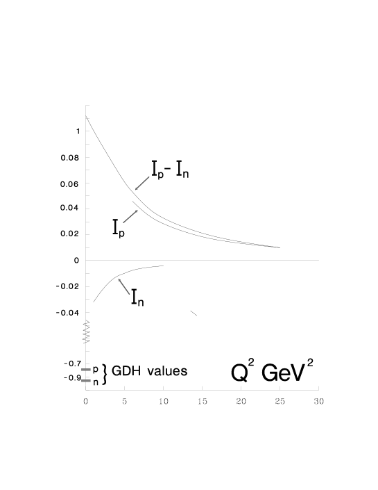
Figure 1:

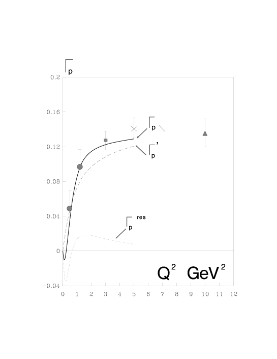
Figure 2:

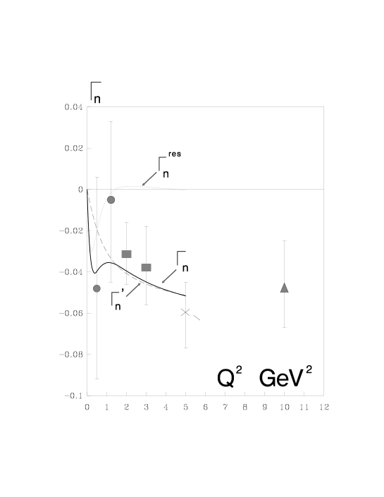
Figure 3:

References

• [1] SMC-Collaboration, hep-ph/9702005, submitted to Physical Review D.
• [2] K.Abe et al (E154 Collab.) Phys.Lett. B405 (1997) 180.
• [3] S.Gerasimov, Yad.Fiz. 2 (1996) 930.
• [4] S.D.Drell and A.C.Hearn, Phys.Rev.Lett. 16 (1996) 908.
• [5] B.L.Ioffe, hep-ph/9704295, Phys.At.Nucl. in press.
• [6] R.M.Barnett et al., Particle Data Group, Phys.Rev. D54 (1996) 1.
• [7] J.Kadaira et al., Phys.Rev. D20 (1979) 627; Nucl.Phys. B159 (1979) 99, 165 (1980) 129.
• [8] S.A.Larin and J.A.M.Vermaseren, Phys.Lett. 259 (1991) 345.
• [9] S.A.Larin, Phys.Lett. 334 (1994) 192.
• [10] S.A.Larin, T.van Ritbergen and J.A.M.Vermaseren, preprint NIKHEF-97-011 (1997).
• [11] A.L.Kataev, Phys.Rev. D50 (1994) 5469.
• [12] S.Y.Hsueh et al., Phys.Rev. D38 (1988) 2056.
• [13] R.D.Carlitz, J.C.Collins and A.H.Mueller, Phys.Lett. B 214 (1988) 229.
• [14] S.D.Bass, B.L.Ioffe, N.N.Nikolaev and A.W.Thomas, J.Moscow Phys.Soc. 1 (1991) 317.
• [15] I.I.Balitsky, V.M.Braun and A.V.Kolesnichenko, Phys.Lett. 242 (1990) 245, Errata B318 (1993) 648.
• [16] A.Oganesian, hep-ph/9704435, Phys.At.Nucl., in press.
• [17] M.J.Alguard et al, Phys.Rev.Lett. 37 (1976) 1261; 41 (1978) 70. G.Baum, ibid 51 (1983) 1135.
• [18] J.Ashman et al, Phys.Lett 206 (1988) 364; Nucl.Phys. B328 (1989) 1.
• [19] K.Abe et al. (SLAC E143 Collaboration), Phys.Rev.Lett. 74 (1995) 346.
• [20] D.Adams et al, Phys.Lett. B329 (1994) 399.
• [21] I.Balitsky, X.Ji, Phys.Rev.Lett. 79 (1997) 1225.
• [22] A.Saalfeld, G.Piller, L.Mankiewicz, Preprint TUM/T39-97-19, hep-ph/9708378.
• [23] M.Anselmino, B.L.Ioffe and E.Leader, Sov.J.Nucl.Phys. 49 (1989) 136.
• [24] V.Burkert and B.L.Ioffe, JETP, 105 (1994) 1153.
• [25] J.Soffer and O.Teryaev, Phys.Rev. D51 (1995) 25.
• [26] B.L.Ioffe, V.A.Khoze, L.N.Lipatov, Hard Processes, v.1, North Holland, Amsterdam, 1984.
• [27] V.Burkert and Z.Li, Phys.Rev. 47 (1993) 46.
• [28] K.Abe et al., (SLAC E143 Collaboration) Phys.Rev.Lett. 78 (1997) 815.
• [29] P.L.Anthony et al. (SLAC E142 Collaboration), Phys.Rev. D54 (1996) 6620.
• [30] K.Abe et al. (SLAC E143 Collaboration), Phys.Rev.Lett. 75 (1995) 25.