The Wilson renormalization group for low x physics:
Gluon evolution at finite parton density.
Jamal Jalilian-Marian¹, Alex Kovner^1,2 and Heribert Weigert^3
1Physics Department, University of Minnesota
Church st. S.E., Minneapolis, MN 55455, USA
²Theoretical Physics, Oxford University, 1 Keble Road, Oxford OX13NP, UK
³ University of Cambridge, Cavendish Laboratory, HEP, Madingley Road,CB3 0HE UK
Abstract

In this paper we derive the complete Wilson renormalization group equation which governs the evolution of the gluon distribution and other gluonic observables at low $x$ and arbitrary density.

1 Introduction

Recent years have seen a surge of activity in the area of the low $x$ physics. Primarily this has been motivated by the new HERA data [1], which has greatly extended the available kinematic region for Deeply Inelastic Scattering (DIS). The data now exists at Bjorken $x$ as low as $10^{-5}$ and it was hoped initially that at such low $x$ and relatively large $Q^{2}$ one would see clearly the new class of perturbative phenomena, those that go under the general name of ”semihard physics”. First, one was hoping to see the unambiguous signs of the perturbative BFKL pomeron [2], which predicts steeply rising gluon distribution (and consequently DIS cross section) as a function of $x$ at fixed $Q^{2}$: $g(x)\propto(1/x)^{4N_{c}\alpha_{s}/\pi}$. Second, it was expected that in this kinematical region the gluon densities will be large enough so that the semihard shadowing effects due to gluon recombination [4] will become sizable.

In actual fact the situation turned out to be not quite so clear cut. The DIS cross section does indeed rise quite steeply with $1/x$. It can be fit by a power of $1/x$, although apparently not as large a power as predicted by the BFKL formula[3]. The GLR parameter $k$ which is the physical parameter for the onset of shadowing was estimated and was indeed found to be close to 1 within the HERA regime [5], which would suggest observable shadowing corrections. Nevertheless, surprisingly enough all the data is described very well by a simple straightforward DGLAP linear evolution [3]. The rise at low $x$ is then a consequence of the standard perturbative evolution of “flat” partonic distributions from a low initial scale $Q^{2}_{0}$ to $Q^{2}$. The shadowing corrections to this perturbative evolution seem to be practically absent. In this sense the higher twist corrections seem to be irrelevant in the HERA regime.

Still it is widely believed that these nonlinear effects must make their presence felt when the partonic densities are high enough. Even if it does not happen in $ep$ collisions at HERA they have a very good chance of being observed in the DIS experiments on nuclei at low $x$ if and when this program takes off at HERA and even more so in the heavy ion collision experiments at LHC. The curious situation with the present HERA data only adds motivation for studying the onset of the shadowing physics.

The shadowing regime can be approached in two ways. Decreasing $Q^{2}$ at fixed (small) $x$ leads to the initial growth of the cross section as $Q^{-2}$. This growth gradually slows down and eventually (almost) stops when the unitarity bound is reached. We will refer to this slow down and the stop of the growth as the shadowing and the saturation respectively. Alternatively one can decrease $x$ at a fixed value of $Q^{2}$. Due to the growth of gluonic distributions the cross section first should exhibit fast growth (powerwise according to the BFKL prediction), which again should slow down and saturate. Our perspective in this paper will be the second one, so that we will be dealing with the evolution of the unintegrated gluon density with $1/x$.

The physics of the nonlinear effects in DIS is basically the physics of dense partonic systems. This statement perhaps needs some clarification. The physical picture of shadowing depends in large measure on the Lorentz frame used to describe the DIS process. In the rest frame of the nucleon the onset of shadowing corrections is due to the multiple scattering processes of the hadronic component of the photon (a quark - antiquark pair) on the nucleon. This can be described by the extension of Glauber multiple scattering formalism to the context of QCD [5]. For multiple scattering to become effective the partonic system does not have to be particularly dense. In this frame the onset of the nonlinearities (multiple scattering) is rather determined by the cross section of the scattering of the hadronic fluctuation on a parton in the nucleon [5]. The authors of Ref.[5] analyzed the corrections to the Glauber formula and concluded that once the rescattering becomes important one also has to take into account corrections due to rescattering of gluons in the cascade produced by the quark - antiquark pair, into which the photon initially fluctuates. The saturation happens in the regime where the gluon density in the photon is high.

In the infinite momentum frame (IMF), where the nucleon carries all the energy prior to collision, the picture is different. Low $x$ here means that one probes low longitudinal momentum - large wavelength fluctuations in the nucleon wave function. These long wavelength gluons are emitted from the valence quarks and gluons in the nucleon. In the standard linear evolution equations (DGLAP or BFKL) the interaction between these wee gluons is disregarded. However when their wave length is large enough, the gluons emitted by different valence partons overlap in space and interact. The first nontrivial effect of this interaction is the recombination process, which slows down the growth of the gluon density and thereby leads to shadowing [4]. The shadowing and saturation in this frame are both clearly effects of large partonic density.

Although the qualitative picture of saturation and unitarization based on the GLR type recombination effects is very appealing, reliable theoretical tools of dealing quantitatively with finite density partonic systems are yet to be developed. The original GLR equation[4, 7] truncates the series in the expansion in powers of density at the first nonlinear term. As all such truncations it has intrinsically a very limited range of validity, since in general one expects that when the first nonlinear term becomes important the higher order terms will be comparable to it in magnitude. The saturation of partonic distributions and restoration of unitarity in high energy (density) limit of QCD is an outstanding problem which remains unsolved although several approaches are being explored in the literature [8, 9, 10].

In this paper we continue to develop a theoretical approach to finite density partonic systems at low $x$. The main goal of this program is to derive the evolution equation for the gluon density at small $x$ without assuming that the density is in any sense small. In the previous papers [11, 12, 13] we have described the main framework of our approach and have discussed several aspects of this evolution. In this work we complete the derivation of the full nonlinear evolution equation.

The present approach is inspired by an idea of McLerran and Venugopalan [14] first formulated in the context of ultrarelativistic heavy ion collisions. The observation in [14] is that there is a regime of high density and weak coupling in which semiclassical methods should apply. It was therefore suggested that the leading small $x$ glue structure of the nucleus is due to the classical gluon field which is created by the random color charges of energetic on-shell partons. The nonlinearities of the Yang - Mills equations exhibit themselves already on this classical level and it is therefore possible that they provide the necessary saturation mechanism at low $x$. This approach assumes that the interaction of the fluctuations of the gluon field is weak. In this sense it is a weak coupling expansion and its validity is therefore restricted to the perturbative “semihard” shadowing effects. It is however nonperturbative in a different sense. In the standard perturbation theory, the charge density is small and the standard perturbative expansion is simultaneously expansion in powers of the charge density. In this language, higher powers of charge density appear as higher twist contributions (although there is no one - to - one correspondence between the twist expansion and expansion in powers of the charge density). The McLerran - Venugopalan (MV) method does not assume expansion in powers of color charge density and corresponds to resummation of a particular type of higher twist terms. In fact the interesting saturation effects are expected when the density is order $\alpha_{s}^{-1}$. This formulation is therefore naturally suited for discussion of the type of problems we are interested in.

Based on this idea the approach was developed which combines the concept of the effective Lagrangian for the low $x$ DIS with the Wilson renormalization group resummation of leading log corrections to the MV approximation [11, 12]. The main effect of the renormalization group procedure is the change in the color charge density distribution in the effective Lagrangian with $1/x$. The RG equation that governs the evolution of this distribution is the subject of the present paper. It was shown in [12] that in the limit of small color charge densities this equation reduces to the celebrated BFKL equation. In [13] we have derived the general form of this evolution equation at finite color charge density. In the present work we calculate the “coefficients” in this renormalization group equation, which are in fact rather “coefficient functions”, thereby providing the last ingredient in the derivation of the full nonlinear evolution equation valid to leading log approximation at finite color charge density. We should stress, that the calculations presented here are only valid to leading order in $\alpha_{s}$. The scale of $\alpha_{s}$ is therefore left undetermined in this framework and the strong interaction coupling constant is treated as a momentum independent constant, just like in the standard BFKL equation. Higher order perturbative calculations of the type of [15] are needed to determine the appropriate scale.

This paper is organized as follows. In Section 2 we motivate and describe the form of the effective Lagrangian for the physics of low $x$ gluons in DIS. In Section 3 we describe in some detail the classical approximation to this effective Lagrangian. It turns out that the proper treatment of this Lagrangian requires careful specification of the complete gauge fixing condition, and this is also done in Section 3. We then discuss the first quantum corrections to the classical approximation which obviate the need for a renormalization group resummation, and the physical interpretation of the change of the color charge density distribution with the RG flow. In Section 4 we describe in detail the Wilson renormalization group procedure as applied to our effective Lagrangian and derive the general form of the RG equation. Section 5 is the central section of this paper. It contains the calculation of the coefficient functions that appear in the RG equation. Finally, Section 6 is devoted to a discussion of our results. Several Appendices contain technical details of the calculation.

We have tried to make this paper self contained, and therefore have included some of the material already contained in the earlier work [11, 12, 13].

2 The Effective Action for Low $x$ DIS.

Throughout this paper we will work in the infinite momentum frame, where the hadron moves in the positive $z$ direction with the velocity close to velocity of light and almost infinite longitudinal momentum $P^{+}\rightarrow\infty$. Also, we will be working in the light cone gauge $A^{+}=0$.

Our task now is to understand the structure of the effective Lagrangian for low $x$ DIS. First, it is well known that the most important degrees of freedom at low $x$ are gluons. In the framework of standard linear evolution equations, the evolution of gluons in the leading approximation is independent of quarks, and the evolution of quarks is entirely driven by the gluonic distribution. We will therefore retain only gluons as our dynamical degrees of freedom and disregard quarks entirely. Importantly, the gluons that we treat as dynamical degrees of freedom are only those which have low longitudinal momentum, lower than some cutoff $\Lambda^{+}=xP^{+}$. Our effective Lagrangian therefore has to be understood as having a built in longitudinal cutoff.

So, what is the Lagrangian that governs the interactions of the low $x$ gluons? First of all, of course it must contain the standard Yang - Mills interaction term

$$-\int\!d^{4}x\ {1\over 4}G^{2}$$ (1)

where $G^{\mu\nu}$ is the gluon field strength tensor

$$G^{\mu\nu}_{a}=\partial^{\mu}A^{\nu}_{a}-\partial^{\nu}A^{\mu}_{a}+gf_{abc}A^{\mu}_{b}A^{\nu}_{c}$$

The gluons with the low longitudinal momentum also interact with the rest of the partons in the hadron, which have larger longitudinal momentum. We will refer to those partons as “fast” for notational convenience, we may think of valence partons as their initial representatives. This interaction certainly can not be neglected, but in the kinematics of IMF and in the light cone gauge it is very simple. The leading interaction is the eikonal vertex $A^{-}J^{+}_{\rm fast}$, where $J^{+}_{\rm fast}$ is the color charge density due to the fast partons.

The dependence of $J^{+}_{\rm fast}$ on $x^{-}$ and $x^{+}$ is very simple. First, since the wavelength of the fast fields is much shorter than that of the dynamical soft gluons the charge they produce is effectively concentrated at $x^{-}=0$. Intuitively this can be understood in the following way. In the rest frame the valence partons are concentrated within the nucleon radius from the center of the nucleon. When boosted to the infinite momentum frame due to Lorentz contraction they are squeezed into a very thin pancake. This picture is a little too naive for our fast partons since some of them have much larger wave length than the nucleon radius. However as a basic physical picture it is still correct. We therefore have $J^{+}\propto\delta(x^{-})$.

Second, we can understand the $x^{+}$ dependence by considering the (light cone) time scales characteristic of the problem. The relevant time scale for the low $x$ phenomena is the inverse of the on shell frequency of the soft gluons: $k^{-}\propto 1/k^{+}$. The frequency of the fast modes is much lower $p^{-}\propto 1/p^{+}$ since their longitudinal momentum is higher, so that $k^{-}/p^{-}\propto 1/x$. Therefore, as far as the soft glue is concerned the color charge source due to fast partons is effectively static. We are therefore led to consider the interaction of the type

$$S_{\rm int}=A^{-}\rho(x_{\perp})\delta(x^{-})$$ (2)

The fast partons are represented in our effective Lagrangian by the surface charge density $\rho(x_{\perp})$. A hadron of course is not described by a fixed single configuration of the color charge density $\rho(x_{\perp})$. However, the crucial point is that the structure of the fast component of the hadron is determined on a much longer time scale than the time scale relevant for the low $x$ physics. It is fixed by the hadronic wave function, bremsstrahlung processes that involve fast partons, etc. Therefore, as far as the soft glue is concerned, there is no interference between the different configurations of $\rho(x_{\perp})$. In the low $x$ effective Lagrangian the hadron thus appears as an ensemble in which different configurations of $\rho(x_{\perp})$ enter with some statistical weight $\exp\{-F[\rho]\}$. The partition function for calculation of the soft glue characteristics of a hadron must therefore have the form

$$\int D[\rho,A]\exp\{-F[\rho]-{i\over 4}\int\!d^{4}x\ G^{2}+iS_{\rm int}[A,\rho]\}$$ (3)

At this point we do not specify the form of the functional $F[\rho]$. In fact, as we shall see later this functional depends on the longitudinal cutoff $\Lambda^{+}$ which is imposed on the soft fields. In other words, as one considers regions of lower and lower $x$, $F$ changes. The flow of $F$ with the cutoff $\Lambda^{+}\propto x$ is described by a renormalization group equation of the form

$${d\over d\ln 1/x}F[\rho]=\alpha_{s}\Delta[\rho]$$ (4)

This RG equation is precisely the evolution equation for the charge density correlators (and consequently for the soft glue observables) which we undertake to derive in this paper.

Of course, in order to make quantitative statements about the $x$ dependence of $F$ we have to specify the initial condition for the evolution. This can be done in the perturbative region at not too small a value of $x$, where $F$ can still be expanded in powers of $\rho$. The initial form of $F$ can then be taken as

$$F=\int dx_{\perp}dy_{\perp}\rho(x_{\perp})\mu^{-1}(x_{\perp},y_{\perp})\rho(y_{\perp})$$ (5)

with

$$\mu(x_{\perp},y_{\perp})=S(b_{\perp})\int{d^{2}k_{\perp}\over(2\pi)^{2}}\ e^{ik_{\perp}(x_{\perp}-y_{\perp})}\,\phi(k_{\perp},x_{0})$$ (6)

Here $b_{\perp}={x_{\perp}+y_{\perp}\over 2}$ is the impact parameter, $S(b_{\perp})$ is a nucleon thickness function, $x_{0}$ is the value of $x$ from which we start evolving $F$ according to the RG equation and $\phi(k_{\perp},x)$ is the unintegrated gluon density. The relation between the parameter in the Gaussian, $\mu^{-1}$ and $\phi$, Eq.(6) will become clear when in Section 3 we consider the perturbative calculation of the gluon structure function based on the effective Lagrangian in Section 2.

One important question that we have not touched upon so far, is the question of gauge invariance of our effective action. Although we have partially fixed the gauge by the light cone gauge condition $A^{+}=0$, the action should still preserve the residual gauge symmetry. This residual gauge symmetry group is comprised of gauge transformations with gauge functions which do not depend of $x^{-}$. The naive “Abelian” eikonal interaction term Eq.(2) does not preserve this gauge symmetry. The relevant generalization takes the form

$$S_{\rm int}={1\over{N_{c}}}\int d^{2}x_{\perp}dx^{-}\delta(x^{-})\rho^{a}(x_{\perp}){\rm tr}T_{a}W_{-\infty,\infty}[A^{-}](x^{-},x_{\perp})$$ (7)

Here $T_{a}$ are the $SU(N)$ color matrices in the adjoint representation and $W$ is the path ordered exponential along the $x^{+}$ direction in the adjoint representation of the $SU(N_{c})$ group

$$W_{-\infty,\infty}[A^{-}](x^{-},x_{\perp})=P\exp\bigg{[}-ig\int dx^{+}A^{-}_{a}(x^{+},x^{-},x_{\perp})T_{a}\bigg{]}$$ (8)

This form is explicitly gauge invariant under the residual gauge transformations with gauge functions which do not depend on $x^{-}$ and vanish at $x^{+}\rightarrow\pm\infty$. Requiring $F[\rho]$ to be gauge invariant, we also restore gauge invariance of the action under the gauge transformations which do not vanish at $x^{+}\rightarrow\pm\infty$ but rather are periodic in $x^{+}$.

This form of the interaction consistently leads to a source term in the corresponding Yang-Mills equation that represents classical colored particles moving along the light cone:

$$D_{\mu}G^{\mu\nu}=J^{+}\delta^{\nu+}$$ (9)

with

$$J^{+}_{a}(x)={g\over{N_{c}}}\delta(x^{-})\rho^{b}(x_{\perp}){\rm tr}\Bigg{[}T_{b}W_{-\infty,x^{+}}[A^{-}]T_{a}W_{x^{+},\infty}[A^{-}]\Bigg{]}$$ (10)

Expanding this expression for the current to lowest order in the field $A^{-}$ yields

$$J^{+}_{a}(x)=g\delta(x^{-})\rho^{a}(x_{\perp})$$ (11)

which reproduces Eq.(2) and is the form of the current used in [14, 16]. As explained in [14], this form is only valid in the gauge $A^{-}(x^{-}=0)=0$. In more general gauges the current has to satisfy the covariant conservation condition

$$D^{-}J^{+}=0$$ (12)

Our current (10) evidently complies with this requirement. This is a direct consequence of the residual gauge invariance.

All of the above considerations finally lead us to the following effective action for the low $x$ DIS

$$S = i\int d^{2}x_{\perp}F[\rho^{a}(x_{\perp})]$$

$$-\int\!d^{4}x\,{1\over 4}G^{2}+{{i}\over{N_{c}}}\int\!d^{2}x_{\perp}dx^{-}\delta(x^{-}){\rm tr}\rho(x_{\perp})W_{-\infty,\infty}[A^{-}](x^{-},x_{\perp})$$

which is the starting point of our approach.

We end this section with a comment about the nature of the action Eq.(2). Although we use the term “effective action” when referring to it, it should be understood that it is different in some important aspects from the “classic” effective Lagrangians, like for example the chiral effective Lagrangian of pion physics. The chiral effective Lagrangian $L[\Pi^{a}]$ describes the dynamics of low momentum pion fields, where the momentum cutoff is determined by the mass of the $\sigma$ - particle, or alternatively the dimensionful pion coupling $f_{\pi}$, $p<4\pi f_{\pi}$. All the modes with momenta above the cutoff, as well as all other heavy excitations of the fundamental theory ($\rho$, $\phi$ mesons, etc.) have been integrated out to arrive at this effective Lagrangian. In this sense our effective Lagrangian is similar. The gluon fields have longitudinal momenta bounded by the cutoff $\Lambda^{+}$, while all higher momentum modes are assumed to have been integrated out.

Importantly, the chiral physics has a sharp scale associated with it - $f_{\pi}$. Consequently, all modes of the pion field with momentum lower than the cutoff are described well by the chiral Lagrangian. In fact, the pions at low momenta interact very weakly, with the strength proportional to $p^{2}/f_{\pi}$. Therefore the perturbation theory in the chiral Lagrangian framework is well behaved and does not lead to large corrections to the tree level results. Also, the description of the low momentum pions is insensitive to the change of the cutoff $\Lambda$.

In our case the situation is very different in this respect. There is no sharp physical separation scale which would separate high from low longitudinal momenta. The separation scale $\Lambda^{+}$ we impose is arbitrary. The interaction does not die away as we go far below $\Lambda^{+}$. Therefore there is no reason to expect that our effective Lagrangian gives an adequate description for the modes with momenta far below the cutoff. In fact, quite to the contrary as we shall see the perturbation theory in our effective theory gives larger corrections the farther we go below the cutoff. In this sense this effective Lagrangian is inadequate for description of momenta $k^{+}\ll\Lambda^{+}$. This is of course the manifestation of the absence of the physical separation scale. This means, that if we want to describe low momenta, $k^{+}\ll\Lambda^{+}$, we have to correct the effective Lagrangian. The arguments presented above however fix the form of all the terms in the Lagrangian apart from $F[\rho]$. If the form of the Lagrangian remains the same under the $k^{+}$ evolution, the only thing that can change is the statistical weight $e^{-F[\rho]}$.

Physically it is quite clear what should happen. As we move to smaller values of the longitudinal momentum $k^{+}$, all the gluons with momenta between $k^{+}$ and $\Lambda^{+}$ are transferred from the category of “soft” (or slow) into the category of “fast”. They cease to be dynamical degree of freedom of interest (hence the dynamical fields have lower cutoff on the longitudinal momentum), but give extra contribution to the static color charge density $\rho(x_{\perp})$. Effectively therefore as we go to lower $x$, the color charge density as seen by the soft glue changes. Since the distribution of the charge density is governed by the statistical weight $e^{-F[\rho]}$, this means that $F$ should change as we lower the longitudinal cutoff $\Lambda^{+}$. This is the physical origin of the renormalization group flow we have referred to earlier. In the following section we will see explicitly how this happens. First, however let us describe how to set up the perturbation theory in the present framework.

3 Perturbative calculation of gluonic observables.

The perturbation theory for the effective Lagrangian Eq.(2) was developed in [14]. It is organized in the following way. First one fixes the configuration of the color charge density, and performs perturbative expansion in $\alpha_{s}$ at fixed $\rho(x_{\perp})$. The charge density is not considered to be small, thus this perturbation theory is different from the standard one in that the calculation is performed in a non vanishing background field. In the second step the averaging over $\rho(x_{\perp})$ should be performed. This part of the calculation is contingent on the knowledge of $F[\rho]$ and is completely nonperturbative. In fact the counterpart of this step in the standard perturbative analysis would be the specification of various gluon operator averages in the hadronic state. Conceptually therefore, the first, perturbative part of the calculation can be thought of as the calculation of the generalized “splitting functions” (which includes however the mixings between operators of different twist and is not intrinsically organized as an expansion in powers of $1/Q^{2}$), while the second, nonperturbative part is parallel to the calculation of operator averages in the hadronic state. In the standard perturbation theory, of course one does not have to know the operator averages in order to derive the evolution equation. As we shall see, the exact same thing happens in our calculation. It is only the perturbative part of the calculation that has to be under control in order to derive the renormalization group equation for $F$. In this section therefore we will discuss the perturbation theory in $\alpha_{s}$ at fixed $\rho(x_{\perp})$.

3.1 The tree level.

As in every perturbative calculation the first step is to find the classical solution to the equations of motion. The equations of motion that follow from the action Eq.(2) are

$$D_{\mu}G^{\mu\nu}={g\over{N_{c}}}\delta(x^{-})\rho^{b}(x_{\perp}){\rm tr}\Bigg{[}T_{b}W_{-\infty,x^{+}}[A^{-}]T_{a}W_{x^{+},\infty}[A^{-}]\Bigg{]}$$ (14)

As explained in the previous section, these equations are invariant under the residual $x^{-}$ independent gauge transformation

$$A\to V\left[A+\frac{i}{g}\partial\right]V^{\dagger}$$ (15)

with

$$V(x)=\exp\left[i\Lambda(x_{\perp},x^{+})\right],\ \ \Lambda\rightarrow_{x^{+}\rightarrow\pm\infty}0$$ (16)

As a consequence, the equations of motion at fixed $\rho$ have an infinite number of solutions. To properly set up perturbation theory, we should choose one of these solutions. Technically this is achieved by gauge fixing the residual gauge freedom. There are of course many possible gauge fixings. From the calculational point of view it is convenient to choose a gauge in which the classical solution is static ($x^{+}$ independent). It is important to realize that the condition of staticity of the classical solution is still insufficient. Even though it completely eliminates the gauge freedom of Eq.(16), there are still many solutions to the equations of motion. This is a consequence of the remaining gauge symmetry of our problem, with gauge functions $\Lambda$ which do not vanish at $x^{+}\rightarrow\pm\infty$, but rather are periodic in $x^{+}$. With the transformation Eq.(16) moded out, those are

$$A\to V\left[A+\frac{i}{g}\partial\right]V^{\dagger}$$ (17)

$$\rho\to V^{\dagger}\rho V$$

$$V(x)=\exp\left[i\Lambda(x_{\perp})\right]$$

To see that this is indeed the case, consider the equations Eq.(14) for static fields (note that all static solutions have vanishing $A^{-}$)

$$\partial_{i}\partial^{+}A^{i}+g[A_{i},\partial^{+}A^{i}]=g\rho(x_{\perp})\delta(x^{-})$$ (18)

$$F^{ij}=0$$

The general solution to this equation has the form

$$A_{i}^{V}[\rho]={i\over g}\theta(x^{-})U(x_{\perp})\partial_{i}U^{\dagger}(x_{\perp})+{i\over g}\theta(-x^{-})V(x_{\perp})\partial_{i}V^{\dagger}(x_{\perp})$$ (19)

where the $SU(N)$ matrices $U$ and $V$ satisfy

$$\partial_{i}\left[V^{\dagger}U\partial_{i}(U^{\dagger}V)\right]=-g^{2}V\rho V^{\dagger}$$ (20)

This equation obviously has a solution for any $V(x_{\perp})$. The matrix $V$, which labels these solutions is closely related to the gauge transformation matrix of Eq.(17), although this relation is rather subtle. Obviously any two solutions Eq.(19), $A_{i}^{V}[\rho]$ and $A_{i}^{V^{\prime}}[\rho]$ are not related by a gauge transformation, since they solve the equation of motion with the same $\rho$, while the gauge transformation Eq.(17) acts nontrivially on $\rho$. However it is easy to see that the set of solutions $\{A_{i}^{V}[\rho]\}$ with fixed $\rho$ and arbitrary $V$ is gauge equivalent to the set of solutions $\{A_{i}^{V^{\prime}}[V^{\dagger}\rho V]\}$ with fixed $V^{\prime}$ (which determines the asymptotics at $x^{-}\rightarrow-\infty$) and arbitrarily rotated $\rho$. Consequently, it would be redundant to take into account all static classical solutions at fixed $\rho$ since we are subsequently performing the unconstrained functional integral over $\rho$ with the measure which is invariant under Eq.(17). We can therefore gauge fix this extra gauge freedom by imposing, for example a fixed boundary condition on $A_{i}$ at $x^{-}\rightarrow-\infty$.

In this paper we will follow Ref.[14] and choose as the subsidiary gauge condition

$$\partial^{i}A_{i}(x^{+},x_{\perp},x^{-}\rightarrow-\infty)=0.$$ (21)

This gauge has a nice feature that at $t\to-\infty$, at all finite values of $z$ (i.e. $x^{-}\to-\infty$) the vector potential is required to be the same as in the perturbative vacuum, $A_{i}=0$. This seems very sensible, since at these times the hadron itself is still at $z\to-\infty$ and could not have changed the quantum state at any finite $z$.

Note that this gauge condition eliminates both, time dependent gauge freedom Eq.(16) and time independent gauge freedom Eq.(17). It is not ghost free, and therefore the measure in the path integral in Eq.(2) must be modified by the appropriate Fadeev-Popov determinant

$$\delta\left(\partial_{i}A_{i}(x^{-}\rightarrow-\infty)\right){\rm det}\left(\partial_{i}D_{i}\left[A_{i}(x^{-}\rightarrow-\infty)\right]\right)$$ (22)

This modification is harmless, since as we will see later the ghosts do not contribute to leading order in $\alpha_{s}$, which is the order to which we calculate.

It is important to realize that the gauge fixing Eq.(21) should be consistently used throughout the whole perturbative calculation. This means that not only does it determine the classical solution we have to pick, but also the form of the propagator of the fluctuations of $A_{\mu}$ around this solution to be used in the higher order perturbative calculations. In this way all potential zero modes in the propagator are eliminated and the calculation is unambiguous. In the standard perturbation theory, although in principle the situation is similar, in practice one can frequently get away without specifying the gauge fixing condition for the residual gauge freedom. The light cone gauge condition $A^{+}=0$ eliminates the major part of the zero mode ambiguity and the rest of the zero modes start causing problems only in higher orders. It turns out that in our calculation we have to be much more careful, and impose the residual gauge fixing properly already in the lowest order. This is related to a nonstandard behavior of our fields at infinity. On the classical level this behavior is obvious from the form of the solution of the equations of motion Eq.(19), which does not vanish at $x^{-}\rightarrow\pm\infty$. We will come back to this question in Section 5.

Returning to Eq.(19) we see that in this gauge for a generic fixed $\rho(x_{\perp})$ there is a unique solution of the form

$$A_{i}=\theta(x^{-})\alpha_{i}(x_{\perp})$$ (23)

$$\alpha_{i}(x_{\perp})={i\over g}U(x_{\perp})\partial_{i}U^{\dagger}(x_{\perp})$$

with the matrix $U(x_{\perp})$ determined by

$$\partial_{i}\alpha_{i}=-g\rho$$ (24)

Any gluonic observable in the tree level approximation is calculated as

$$<O[A_{\mu}]>=\int D[\rho]e^{-F[\rho]}\ O\left[A^{-}=0,A_{i}=\theta(x^{-})\alpha_{i}[\rho]\right]$$ (25)

For example, the unintegrated gluon density defined as

$$g(x,k_{\perp})=<\hat{a}^{\dagger a}_{\lambda}(x,k_{\perp})\hat{a}^{a}_{\lambda}(x,k_{\perp})>$$ (26)

where $\hat{a}$ and $\hat{a}^{\dagger}$ are the light cone gluon creation and annihilation operators, is given by

$$g(x,k_{\perp})={1\over x}<\alpha_{i}^{a}(k_{\perp})\alpha_{i}^{a}(-k_{\perp})>$$ (27)

Here the $<\ >$ denotes averaging over $\rho$ with the weight $\exp\{-F\}$.

This has a simple representation in terms of the standard Feynman diagrams. The classical field is given by the sum of the tree diagrams for one point function in the background density. Using curly lines to represent gluons we have the following graphical representation for the full classical solution $b$ and the first few terms in its pertrubative expansion

$$b = \begin{minipage}[c]{56.9055pt} \psfig{width=56.9055pt} \end{minipage}=\begin{minipage}[c]{28.45274pt} \psfig{width=28.45274pt} \end{minipage}\ {g\rho}+g\ \begin{minipage}[c]{51.21504pt} \psfig{width=51.21504pt} \end{minipage}\begin{minipage}[c]{28.45274pt} ${g\rho}$\\ \vskip 42.67912pt${g\rho}$ \end{minipage}+{\cal O}(\rho^{3})$$ (28)

The distribution function (up to some simple kinematical factors) is just the square of the field averaged over $\rho$. To the order $\rho^{2}$ it is related in a simple way to the color charge density correlation function

$$g(x,k_{\perp}) = {1\over xk^{2}_{\perp}}<\rho(k_{\perp})\rho(-k_{\perp})>$$ (29)

$$= <\partial^{i}\ \begin{minipage}[c]{34.14322pt} \psfig{width=34.14322pt} \end{minipage}\hskip 5.69046pt\cdot\hskip 5.69046pt\partial^{i}\ \begin{minipage}[c]{34.14322pt} \psfig{width=34.14322pt} \end{minipage}+{\cal O}(\rho^{3})>$$

where we have drawn the factors of $\rho$ as diagonal lines to indicate that they are always associated with eikonal lines along the $x^{+}$ direction that correspond to the worldlines of the fast particles they represent.

We stress that our goal in this paper is to perform the calculation to all orders in $\rho$ in the first order in $\alpha_{s}$. Hence an expansion in powers of $\rho$ as in Eqns. (28) and (29) would not be sufficient for our purpose. However, the above representations are helpful in visualizing the physical mechanism underlying the running of the charge density distribution with $1/x$. Also, even though our interest is in the phenomenon of shadowing and saturation, which occur at large $\rho$, our calculational procedure should be valid also at small color charge density. In this limit we should recover the known perturbative results, which in the present context is the BFKL equation. Expansion to leading order in $\rho$ of our result will therefore be an important consistency check in the calculation.

3.2 The first order perturbative corrections.

One prominent feature of Eq.(27) is the full tree level $x$ dependence of the gluon density. It is precisely the same as in the leading order in the standard perturbation theory. We know, that in the standard calculation this lowest order $x$ dependence feeds back through the higher order graphs and leads to large perturbative corrections at small $x$. We expect therefore that the same will happen in our perturbation theory. Indeed, consider for example the graph on Fig.1b, which gives one of the contributions to the gluon density at order $\alpha_{s}$.

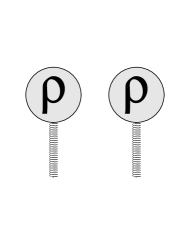
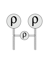
(a)	(b)

Figure 1: Diagram contributing to the gluon distribution at lowest order in $\alpha_{s}$ (but to all orders in $\rho$) (a) and a typical order $\alpha_{s}$ correction (b). The horizontal line represents a propagator in the presence of the full, $\rho$-induced background field

(a)	(b)

Figure 2: The small $\rho$ limit of the diagrams shown in Fig. 1: The lowest order terms shown in (a) correspond to those in Eq.(29). (b) is the small $\rho$ limit of Fig.1b with all gluon propagators perturbative.

This contribution was discussed in [16], and it was shown there that it is indeed of order $\alpha_{s}\ln(1/x)$ relative to the leading order result Eq.(27), or in the low density limit, Eq.(29). The reason for this enhancement is that when the momentum on the external leg $l^{+}$ is much smaller than the maximal longitudinal momentum allowed in the field, there is huge phase space available to the emitted gluon $l^{+}<k^{+}<\Lambda^{+}$. The phase space integral $\int{dk^{+}\over k^{+}}$ then gives the logarithmic enhancement factor.

Carefully examining the $\alpha_{s}\ln 1/x$ corrections of Figs. 1b, 2b , we see that it looks very similar to the tree level diagrams of Figs. 1a, 2a, except that the soft gluon is emitted not from the original charge density $\rho$ as depicted in Fig.3a, but rather from a modified charge density which in addition to $\rho$ contains one extra gluon. One therefore can think of it as being emitted from the modified vertex of Fig.3b. Since the large correction comes from the region $l^{+}\ll k^{+}$, the emission from the modified vertex is also eikonal.

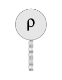
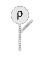
$l^{+}$	$k^{+}$ $l^{+}$
(a)	(b)

Figure 3: Original vertex (a) and vertex modified by the emission of an additional fast gluon (b). “$+$” components of momenta are ordered from top to bottom

So the source for emission of very soft gluons with $l^{+}\ll\Lambda^{+}$ effectively has been modified. This modification has to be taken into account if we are to describe properly the soft glue distribution. Fortunately, the change in the charge density is slow (logarithmic) so that this is a perfect situation for the application of the Wilson renormalization group ideas. We can integrate out the fluctuations around the classical background perturbatively, gradually lowering the longitudinal momentum cutoff $\Lambda^{+}$ on the remaining dynamical degrees of freedom. This will generate the effective Lagrangian below the new cutoff scale with modified $F[\rho]$. So long as we keep the change in the cutoff in every step of the RG small enough so that the correction to $F$ is small relative to $F$ itself, the perturbative procedure is justified. The condition for that is $\ln{\Lambda^{+}-\delta\Lambda^{+}\over\Lambda^{+}}\sim 1$, $\alpha_{s}\ln{\Lambda^{+}-\delta\Lambda^{+}\over\Lambda^{+}}\ll 1$. In the next section we describe in detail how to set up this renormalization group procedure.

4 The low x Wilson renormalization group.

Let us introduce the following decomposition of the gauge field:

$$A^{a}_{\mu}(x)=b^{a}_{\mu}(x)+\delta A^{a}_{\mu}(x)+a^{a}_{\mu}(x)$$ (30)

where $b^{a}_{\mu}(x)$ is the solution of the classical equations of motion Eq.(23), $\delta A^{a}_{\mu}(x)$ is the fluctuation field containing longitudinal momentum modes $q^{+}$ such that $\Lambda^{+}-\delta\Lambda^{+}\equiv\Lambda^{+^{\prime}}<q^{+}<\Lambda^{+}$ while $a$ is a soft field with momenta $k^{+}<\Lambda^{+^{\prime}}$. Our aim is to integrate out the fluctuation field $\delta A_{\mu}$ in the path integral and compute the effective action for the soft field $a_{\mu}$ This integration is performed within the assumption that the fluctuations are small as compared to the classical fields $b^{a}_{\mu}$. More quantitatively, this requires that the coupling constant is small $\alpha_{s}\ll 1$ and at each step of the renormalization group procedure the ratio of the two cutoffs is not too big, $\ln{\Lambda^{+}\over\Lambda^{+^{\prime}}}\ll{1\over\alpha_{s}}$

To leading order in the coupling constant we should only keep the terms up to second order in the fluctuation field $\delta A_{\mu}$ in the expansion of the action around the classical solution $b^{a}_{\mu}(x)$.

$$S=-{1\over 4}G(a)^{2}-{{1}\over{2}}\delta A_{\mu}[{\rm D}^{-1}(\rho)]^{\mu\nu}\delta A_{\nu}+ga^{-}J^{+\prime}+O((a^{-})^{2})+iF[\rho]$$ (31)

The inverse propagator of the fluctuation, $[{\rm D}^{-1}(\rho)]^{\mu\nu}$ has a nontrivial dependence on the color charge density. Its explicit form is given in the next section, Eq.(56).

We have introduced the modified color charge current $J^{+\prime}$, whose explicit form in terms of the fluctuation fields is

$$J^{+\prime}=\rho(x_{\perp})\delta(x^{-})+\delta J^{+}_{1}+\delta J^{+}_{2}$$ (32)

with

$$\delta J^{+a}_{1}(x_{\perp},x^{+})=\delta(x^{-})\Bigg{[}-2f^{abc}\alpha^{b}_{i}\delta A^{c}_{i}(x^{-}=0)-{{g}\over{2}}f^{abc}\rho^{b}(x_{\perp})$$

$$\hskip 56.9055pt\times\int\!dy^{+}\Bigg{[}\theta(y^{+}-x^{+})-\theta(x^{+}-y^{+})\Bigg{]}\delta A^{-c}(y^{+},x^{-}=0)\Bigg{]}$$

and

$$\delta J^{+a}_{2}(x)=-f^{abc}[\partial^{+}\delta A^{b}_{i}(x)]\delta A^{c}_{i}(x)-{{g^{2}}\over{N_{c}}}\rho^{b}(x_{\perp})\delta(x^{-})$$

$$\hskip 28.45274pt\times\int dy^{+}\delta A^{-c}(y^{+},x_{\perp},x^{-}=0)\int dz^{+}\delta A^{-d}(z^{+},x_{\perp},x^{-}=0)$$

$$\hskip 28.45274pt\times\Bigg{[}\theta(z^{+}-y^{+})\theta(y^{+}-x^{+}){\rm tr}T^{a}T^{c}T^{d}T^{b}$$

$$\hskip 34.14322pt+\theta(x^{+}-z^{+})\theta(z^{+}-y^{+}){\rm tr}T^{a}T^{b}T^{c}T^{d}$$

$$\hskip 34.14322pt+\theta(z^{+}-x^{+})\theta(x^{+}-y^{+}){\rm tr}T^{a}T^{d}T^{b}T^{c}\Bigg{]}$$

The first term in both $\delta J_{1}^{+a}$ and $\delta J^{+a}_{2}$ arises from the expansion of $G^{2}$ in the action while the rest of the terms proportional to $\rho(x_{\perp})$ are coming from the expansion of the Wilson line term. The various terms with $\theta$ functions correspond to different time orderings of the fields along the Wilson lines. Since the longitudinal momentum of $a^{-}$ is much lower than of $\delta A$, we have only kept the eikonal coupling (the coupling to $a^{-}$ only), which gives the leading contribution in this kinematics. The contributions to $\delta J_{1}$ and $\delta J_{2}$ are depicted in Fig.4 and 5 respectively. Obviously the first diagram in Fig.4 is nothing but our modified vertex of Fig.3b, now cast in a more precise language. All other terms are nontrivial consequences of the presence of a background of fast “classical” particles that are encoded in the source term $\rho$ and a careful treatment of the path integral over the modes in the interval $[\Lambda^{+},\Lambda^{\prime+}]$.

$$\begin{minipage}{85.35826pt} \psfig{width=59.75095pt} \end{minipage}\circ\delta A+\begin{minipage}{85.35826pt} \psfig{width=85.35826pt} \end{minipage}\circ\delta A+\begin{minipage}{62.59596pt} \psfig{width=61.17325pt} \end{minipage}\circ\delta A$$

Figure 4: Diagrammatic representation of $\delta J_{1}$ in terms of classical and fluctuation fields. The coupling to a $\delta A_{\mu}$ field has been indicated by a curly line whereas slow modes $a_{\mu}$ have been symbolized by dashed ones.

$\delta A$ $\delta A$

+  $\delta A$$\delta A$
+ different time orderings

Figure 5: Diagrammatic representation of $\delta J_{2}$. Symbols as in Fig.4

We have not written out explicitly higher order in $a^{-}$ terms in the effective action. There are of course such terms, which come from expanding the Wilson line part of the action. Disregarding these terms gives the effective action with the coupling of the field $a^{-}$ to the charge density of the form $a^{-}J^{+}$. However, imposing gauge invariance on the final result together with the requirement that the linear in $a^{-}$ term of the gauge invariant action should coincide with the result of our calculation, the full gauge invariant form of the effective action will be recovered. In the following therefore we will concentrate on the linear term $a^{-}J^{+}$ only. Note that the first term in Eq.(4) does not have an explicit factor of $\delta(x^{-})$. However we are only interested in its low longitudinal momentum components since it couples directly to $a^{-}$ in the effective action. In momentum space this contribution is given by $f^{abc}\int dq^{+}[q^{+}\delta A^{b}_{i}(q^{+})]\delta A^{c}_{i}(-q^{+}+k^{+})$. Since the leading logarithmic contributions comes from the region $q^{+}\gg k^{+}$, to this accuracy this expression does not depend on $k^{+}$ and can be therefore approximated by $\delta(x^{-})$ in coordinate space. We then can define the modified surface color charge density by

$$\delta J^{+}(x_{\perp},x^{-})=\delta\rho(x_{\perp})\delta(x^{-})$$

$$\delta\rho(x_{\perp})=\int\!dx^{-}\delta J^{+}(x_{\perp},x^{-})$$ (35)

Formally $\delta\rho$ defined in this way is a function of $x^{+}$ as well as $x_{\perp}$. However, it is a function of $\delta A$’s which only have longitudinal momenta much larger than the momenta in the soft field $a$. The (light cone) time variation scale of $\delta\rho$ is therefore ${1\over q^{-}}\sim{q^{+}\over q_{\perp}^{2}}$ and is much larger than the typical time variation scale of the on shell modes of the field $a$. From this point of view $\delta\rho$ is therefore for all practical purposes (light cone) time independent. Technically this means that whenever we will need a correlation function of $\delta\rho$’s, we will expand it to leading order in the time derivatives

$$<\delta\rho(x_{\perp},x^{+})\delta\rho(y_{\perp},y^{+})>=<\delta\rho(x_{\perp},x^{+})\delta\rho(y_{\perp},x^{+})>+...$$ (36)

Corrections to this approximation are of order $q^{-}/k^{-}\sim x$. We will therefore not indicate the time dependence of $\rho$ explicitly.

The procedure now is the following. We first introduce the variable $\rho^{\prime}$ in the path integral by

$$\int\!\!D[\rho,\delta A_{\mu},a_{\mu}]e^{iS[a_{\mu},\delta A_{\mu},\rho]}=\int\!\!D[\rho^{\prime},\rho,\delta A_{\mu},a_{\mu}]\delta(\rho^{\prime}-\rho-\delta\rho[\delta A])e^{iS[a_{\mu},\delta A_{\mu},\rho]}$$ (37)

Here $\delta\rho[\delta A]$ is the functional of the fluctuation fields defined by Eqs.(4,4,4). Now we first have to integrate $\delta A_{\mu}$ at fixed $\rho$, and then integrate over $\rho$.

This procedure generates the new effective action which symbolically can be written as

$$\exp\{iS[\rho^{\prime},a^{\mu}]\}=\exp\{-F^{\prime}[\rho^{\prime}]-{i\over 4}G^{2}(a)+iga\rho^{\prime}\}$$ (38)

with

$$\exp\{-F^{\prime}[\rho^{\prime}]\}=\int D[\rho,\delta A]\ \delta(\rho^{\prime}-\rho-\delta\rho[\delta A])\exp\{-F[\rho]-{i\over 2}\delta AD^{-1}[\rho]\delta A\}$$ (39)

Of course, to leading order in $\ln 1/x$ only terms linear in $\alpha_{s}\ln 1/x$ should be kept in $F^{\prime}$.

The integration over the fluctuation field $\delta A_{\mu}$ is the most technically involved part of this procedure. We will describe in detail this part of the calculation in the next section. The structure of the result is however easy to understand from a simple counting of powers of the coupling constant $\alpha_{s}$. Consider integration over the fluctuation field $\delta A_{\mu}$ at fixed $\rho$. The counting of the powers of $\alpha_{s}$ is done most conveniently after rescaling the fields and the charge density in the following way:

$$A_{\mu}\rightarrow{1\over g}A_{\mu}$$ (40)

$$\rho\rightarrow{1\over g^{2}}\rho$$

$$\delta\rho\rightarrow{1\over g^{2}}\delta\rho$$

Explicitly for the rescaled charge density we have

$$\rho^{+\prime}=\rho(x_{\perp})+\delta\rho^{+}_{1}+\delta\rho^{+}_{2}$$ (41)

with

$$\delta\rho^{+a}_{1}(x_{\perp}) = -2f^{abc}\alpha^{b}_{i}\delta A^{c}_{i}(x^{-}=0)-{{1}\over{2}}f^{abc}\rho^{b}(x_{\perp})$$

$$\hskip 14.22636pt\times\int dy^{+}\Bigg{[}\theta(y^{+}-x^{+})-\theta(x^{+}-y^{+})\Bigg{]}\delta A^{-c}(y^{+},x_{\perp},x^{-}=0)$$

and

$$\delta\rho^{+a}_{2}(x) = -f^{abc}\int dx^{-}[\partial^{+}\delta A^{b}_{i}(x)]\delta A^{c}_{i}(x)$$ (44)

$$+{1\over{N_{c}}}\rho^{b}(x_{\perp})\int\!dy^{+}\delta A^{-c}(y^{+},x_{\perp},x^{-}=0)$$

$$\hskip 28.45274pt\times\int\!dz^{+}\delta A^{-d}(z^{+},x_{\perp},x^{-}=0)$$

$$\hskip 28.45274pt\times\Bigg{[}f^{ace}f^{bde}\theta(z^{+}-x^{+})\theta(x^{+}-y^{+})\Bigg{]}$$

with

$$\alpha_{i}(x_{\perp}) = iU(x_{\perp})\partial_{i}U^{\dagger}(x_{\perp})$$

$$\partial_{i}\alpha_{i} = -\rho$$ (45)

In terms of the rescaled fields the coupling constant $g$ disappears from the expressions for $\delta\rho$, and appears only as the overall factor $1/g^{2}$ in the action. The propagator of the fluctuation field is therefore of order $\alpha_{s}$. It immediately follows from Eqs.(4) and (44 that

$$<\delta\rho>_{\delta A}=O(\alpha_{s})$$

$$<\delta\rho\delta\rho>_{\delta A}=O(\alpha_{s})$$ (46)

while all other (connected) correlation functions of $\delta\rho$ are higher order in $\alpha_{s}$. Since we are working to the lowest order in $\alpha_{s}$ we can neglect all these other terms. Therefore to lowest order in $\alpha_{s}$, after integrating over $\delta A$ at fixed $\rho$, we are left with the weight function for $\delta\rho$, which generates only connected one- and two-point functions. Such weight is obviously a Gaussian. Introducing the following notations

$$<\delta\rho^{a}(x_{\perp})>_{\delta A}=:\alpha_{s}\ln{1\over x}\sigma^{a}(x_{\perp})$$

$$<\delta\rho^{a}(x_{\perp},x^{+})\delta\rho^{b}(y_{\perp},x^{+})>_{\delta A}=:\alpha_{s}\ln{1\over x}\chi^{ab}(x_{\perp},y_{\perp})$$ (47)

we can write the result of the $\delta A_{\mu}$ integration in the form

$$\int D[\rho,\rho^{\prime}][{\rm Det}(\chi)]^{-1/2}\exp\left(-F[\rho]\right)$$

$$\times\exp\left(-{1\over 2\,\alpha_{s}\,ln{1\over x}}\left[\rho^{\prime}_{x}-\rho_{x}-\alpha_{s}\ln{1\over x}\sigma_{x}\right][\chi^{-1}_{xy}]\left[\rho^{\prime}_{y}-\rho_{y}-\alpha_{s}\ln{1\over x}\sigma_{y}\right]\right)$$

In the above equation we adopted condensed notations: the indices $x$ stand for the set of indices and coordinates $\{x_{\perp},a\}$, and repeated indices are understood to be summed (integrated) over.

The calculation of $\chi$ and $\sigma$ is the subject of the following section. However, the knowledge of the general structure of the $\rho$ integral, Eq.(4) is sufficient to perform the integral over $\rho$ in Eq.(39) without the explicit knowledge of $\chi$ and $\sigma$. The reason is that the integrand in Eq.(4) is a function very sharply peaked around $\rho=\rho^{\prime}+O(\alpha_{s}$), and the integral is calculable in the steepest descent approximation. This was done in [13]. The result is very simple

$$F^{\prime}=F+{\alpha_{s}\ln(1/x)\over 2}\left[\chi_{uv}{\delta^{2}\over\delta\rho_{u}\delta\rho_{v}}F-{\delta^{2}\chi_{uv}\over\delta\rho_{u}\delta\rho_{v}}-{\delta F\over\delta\rho_{u}}\chi_{uv}{\delta F\over\delta\rho_{v}}\right.$$

$$\left.\hskip 28.45274pt+2{\delta F\over\delta\rho_{u}}{\delta\chi_{uv}\over\delta\rho_{v}}+2{\delta\sigma_{u}\over\delta\rho_{u}}-2{\delta F\over\delta\rho_{u}}\sigma_{u}\right]$$ (50)

Taking the derivative with respect to $\ln 1/x$ we obtain the Wilson renormalization group equation for the functional $F$

$${d\over d\ln(1/x)}F = {\alpha_{s}\over 2}\left[\chi_{uv}{\delta^{2}\over\delta\rho_{u}\delta\rho_{v}}F-{\delta^{2}\chi_{uv}\over\delta\rho_{u}\delta\rho_{v}}-{\delta F\over\delta\rho_{u}}\chi_{uv}{\delta F\over\delta\rho_{v}}\right.$$ (51)

$$\left.\hskip 28.45274pt+2{\delta F\over\delta\rho_{u}}{\delta\chi_{uv}\over\delta\rho_{v}}+2{\delta\sigma_{u}\over\delta\rho_{u}}-2{\delta F\over\delta\rho_{u}}\sigma_{u}\right]$$

This equation is extremely simple when written for the weight function $Z\equiv\exp\{-F\}$

$${d\over d\ln(1/x)}Z=\alpha_{s}\left\{{1\over 2}{\delta^{2}\over\delta\rho_{u}\delta\rho_{v}}\left[Z\chi_{uv}\right]-{\delta\over\delta\rho_{u}}\left[Z\sigma_{u}\right]\right\}$$ (52)

Equations (51) and (52) provide the closed form of the renormalization group equation in terms of the functionals $\sigma[\rho]$ and $\chi[\rho]$. In the next section we will calculate these two quantities.

Eq.(52) can be written directly as evolution equation for the correlators of the charge density. Multiplying Eq.(52) by $\rho_{x_{1}}...\rho_{x_{n}}$ and integrating over $\rho$ yields

$${d\over d\ln(1/x)}<\rho_{x_{1}}...\rho_{x_{n}}>$$

$$=\alpha_{s}\left[\sum_{0<m<k<n+1}<\rho_{x_{1}}...\rho_{x_{m-1}}\rho_{x_{m+1}}...\rho_{x_{k-1}}\rho_{x_{k+1}}...\rho_{x_{n}}\chi_{x_{m}x_{k}}>\right.$$

$$\left.\hskip 28.45274pt+\sum_{0<l<n+1}<\rho_{x_{1}}...\rho_{x_{l-1}}\rho_{x_{l+1}}...\rho_{x_{n}}\sigma_{x_{l}}>\right]$$

In particular, taking $n=2$ we obtain the evolution equation for the two point function

$${d\over d\ln(1/x)}<\rho_{x}\rho_{y}>=\alpha_{s}\left\{<\chi_{xy}+\rho_{x}\sigma_{y}+\rho_{y}\sigma_{x}>\right\}$$ (54)

This equation is useful in making contact with standard evolution equations, since the correlator of the color charge density at weak fields is directly related to the unintegrated gluon density in a hadron [12]. Eq. (54) can then be straightforwardly rewritten as an evolution equation for the gluon density.

5 Small fluctuations in the background field. The calculation of $\sigma$ and $\chi$.

In this section we calculate the one - point function $\sigma$ and two - point correlation function $\chi$ of $\delta\rho(x_{\perp})$, Eq.(4), (44). First, note that these quantities are given by the Feynman diagrams of Fig.6 and 7 respectively.

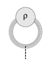
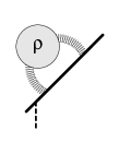
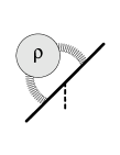
Figure 6: Diagrams contributing to $\sigma$. Note that these are all virtual contributions resulting from contracting the $\delta A$ lines of the diagrams shown in Fig.5

$$\left(\begin{minipage}{29.87547pt} \psfig{width=29.87547pt} \end{minipage}+\begin{minipage}{42.67912pt} \psfig{width=42.67912pt} \end{minipage}+\begin{minipage}{31.2982pt} \psfig{width=31.2982pt} \end{minipage}\right)\circ\begin{minipage}{42.67912pt} \psfig{width=42.67912pt} \end{minipage}\circ\left(\begin{minipage}{29.87547pt} \psfig{width=29.87547pt} \end{minipage}+\begin{minipage}{31.2982pt} \psfig{width=31.2982pt} \end{minipage}+\begin{minipage}{42.67912pt} \psfig{width=42.67912pt} \end{minipage}\right)$$

Figure 7: Diagrams contributing to $\alpha_{s}\ln 1/x\chi$. Note that these arise from contracting to factors of the diagrams shown in Fig.4. For a separate list of all 9 contributions see Fig.8

The propagator lines in these diagrams are the propagators of the fluctuation fields $\delta A$ in the non vanishing background. This is the inverse of the operator $D^{-1}_{\mu\nu}$ that appears in Eq.(31).

At this point we see that the ghosts associated with our gauge fixing do not contribute to order $\alpha_{s}$. The interaction of the ghost fields with the rescaled fluctuation field is order one, see Eq.(22). However any insertion of a ghost vertex will lead to an extra fluctuation propagator and this is proportional to $\alpha_{s}$. We therefore forget about ghosts from now on.

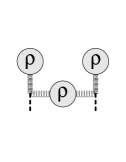
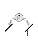
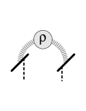
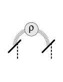
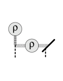
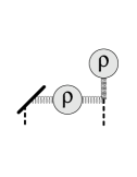
Figure 8: Explicit list of the diagrams contributing to $\chi$

Our goal therefore would seem to be the inversion of $D^{-1}_{\mu\nu}$. In fact our task is a little simpler than that, since we only need to calculate the time independent average in $\sigma$ and the equal time correlator in $\chi$. Those are determined by the Wightman function of the fluctuation field $D_{W}$ rather than by the Feynman propagator. The Wightman function satisfies the homogeneous equation

$$D^{-1}D_{W}=0$$ (55)

and is constructed from the eigenfunctions of $D^{-1}$ with the zero eigenvalue. Our first task is therefore to find the zero eigenfunctions of $D^{-1}$. For completeness we will present also the eigenfunctions with nonzero eigenvalues, but will not construct explicitly the Feynman propagator.

For clarity we have split our calculation into three main parts. We determine the eigenfunctions in subsection 5.1, find their proper normalization in subsection 5.2 and use these results to express the main quantities of interest, $\chi$ and $\sigma$ in subsection 5.3, Eqs.(5.3) and (108)

5.1 The eigenfunctions of $D^{-1}_{\mu\nu}$.

The quadratic action for the fluctuation fields is

$$S=\frac{1}{2g^{2}}\Bigg{\{}a^{-}_{x}K_{xy}a^{-}_{y}+2a^{-}(\partial^{+}Da+2fa)+2\partial^{+}a_{i}\partial^{-}a_{i}+-a_{i}\bigg{[}D^{2}\delta_{ij}+D_{i}D_{j}\bigg{]}a_{j}\Bigg{\}}$$ (56)

Here we are using the following condensed notation

$$[fa]^{a}(x^{+},x^{-},x_{\perp})=f^{abc}\delta(x^{-})\alpha^{ic}(x_{\perp})a^{ib}(x^{+},x^{-},x_{\perp})$$

$$Da=D_{i}[\alpha]a_{i}=(\partial_{i}\delta^{ab}+f^{abc}\theta(x^{-})\alpha_{i}^{c})a^{b}_{i}$$ (57)

and $x$ denotes the space time coordinates $x^{\pm},x^{i}$ as well as color label. All repeated indices are summed (integrated) over. The function $\alpha_{i}(x_{\perp})$ is related to $\rho(x_{\perp})$ through Eq.(4). The operator $K$ is

$$K^{ab}_{xy} = -\bigg{[}(\partial^{+})^{2}\delta^{ab}+f^{abc}\rho^{c}\delta(x^{-})\frac{1}{\partial^{-}}\bigg{]}$$ (58)

$$= -\bigg{[}(\partial^{+})^{2}\delta^{ab}-2M^{ab}\delta(x^{-})\bigg{]}$$

where we have defined

$$M^{ab}(p^{-},x_{\perp})={i\over 2p^{-}}f^{abc}\rho^{c}(x_{\perp})\equiv{if\cdot\rho(x_{\perp})\over 2p^{-}}$$ (59)

Note, that $M$ is a color matrix locally defined in the transverse and frequency space, which does not depend on $x^{-}$.

For simplicity we will temporarily omit the factor $1/g^{2}$ in front of the action, remembering to restore it in the expressions for the charge density by appropriately scaling the small fluctuations propagator.

We have changed our notations from the previous section and denote the fluctuation field by $a_{\mu}$ rather than $\delta A_{\mu}$. We should remember that the fluctuation fields contain longitudinal momenta only above some scale $\Lambda^{+^{\prime}}$. The question how exactly to impose this cutoff is unimportant in the leading logarithmic approximation. We find convenient to introduce it through the infrared cutoff in coordinate space. The longitudinal coordinate $x^{-}$ in our expressions therefore varies between $-L$ and $L$. Whenever it is harmless, we will take the limit $L\rightarrow\infty$, which corresponds to the big cutoff ratio $\Lambda^{+}/\Lambda^{+^{\prime}}\gg 1$.

Rather than writing down the eigenvalue equations for the quadratic Lagrangian Eq.(56) it is more convenient first to explicitly decouple the $a^{-}$ field. This is done by completing the square in Eq.(56)

$$S = \frac{1}{2}\bigg{\{}\bigg{[}a^{-}+K^{-1}(\partial^{+}Da+2fa)\bigg{]}_{x}K_{xy}\bigg{[}a^{-}+K^{-1}(\partial^{+}Da+2fa)\bigg{]}_{y}$$

$$- \bigg{[}\partial^{+}Da+2fa\bigg{]}_{x}K^{-1}_{xy}\bigg{[}\partial^{+}Da+2fa\bigg{]}_{y}+2\partial^{+}a_{i}\partial^{-}a_{i}-a_{i}\bigg{[}D^{2}\delta_{ij}+D_{i}D_{j}\bigg{]}a_{j}\bigg{\}}$$

Defining

$$\tilde{a}^{-}=a^{-}+K^{-1}(\partial^{+}Da+2fa)$$ (61)

we see that it decouples from $a_{i}$. Its correlator is given by

$$<\tilde{a}^{-}_{x}\tilde{a}^{-}_{y}>=K^{-1}_{x,y}$$ (62)

The correlator of $a^{-}$ is then easily calculable once we know $K^{-1}$ and the correlators of $a_{i}$.

The calculation of $K^{-1}$ is straightforward and is given in Appendix A. The result is

$$K^{-1}=\Bigg{\{}-{1\over 2}|x^{-}-y^{-}|+{1\over 2}\eta(x_{\perp})\bigg{[}|x^{-}|+|y^{-}|\bigg{]}-{\eta(x_{\perp})\over 2M}\Bigg{\}}\delta(x_{\perp},y_{\perp})$$ (63)

The color matrix $\eta^{ab}(x_{\perp})$ projects onto the nonzero eigenvalue subspace of $M$. Together with the complementary projector $\mu$ it satisfies the relations

$$\mu M=0,\;\;\;\eta M=M$$ (64)

and

$$\mu+\eta=1,\;\;\mu^{2}=\mu,\;\;\eta^{2}=\eta$$ (65)

We note, that the operator $K$ Eq.(58) has zero modes of the form

$$f^{a}(x_{\perp},x^{-},p^{-})=\mu^{ab}f(x_{\perp},p^{-})$$ (66)

and is therefore strictly speaking non invertible. The result Eq.(63) was obtained by excluding the zero modes and inverting $K$ on the space of functions which does not include the functions Eq.(66). The normalizable zero modes of $K$ can not be completely neglected in Eq.(56). Expanding $a^{-}$ in the basis of eigenfunctions of $K$

$$a^{-}=\int d\lambda a^{-}_{\lambda}f_{\lambda}$$ (67)

we see immediately that $a^{-}_{0}$ drops out from the first term in Eq.(56) but not from the second term. As a result $a^{-}_{0}$ does not decouple from $a_{i}$ and the Eq.(5.1) should be slightly modified. In addition to the term quadratic in $\tilde{a}^{-}$ we have

$$S = -{1\over 2}\bigg{[}\partial^{+}Da+2fa\bigg{]}_{x}K^{-1}_{xy}\bigg{[}\partial^{+}Da+2fa\bigg{]}_{y}+\partial^{+}a_{i}\partial^{-}a_{i}-{1\over 2}a_{i}\bigg{[}D^{2}\delta_{ij}+D_{i}D_{j}\bigg{]}a_{j}$$ (68)

$$+a^{-}_{0,x_{\perp},x^{+}}\mu_{x_{\perp}}\int dx^{-}\bigg{[}\partial^{+}Da+2fa\bigg{]}_{x}$$

Note that $a^{-}_{0}$ does not depend on $x^{-}$ since the zero mode of $K$ is constant in $x^{-}$. The linear term in $a^{-}$ in Eq.(68) is in fact nothing but the Gauss’ law constraint which remains after integrating out the $a^{-}$ component of the vector potential. As we stressed before, our effective Lagrangian is gauge invariant under the residual $x^{-}$ independent non-Abelian gauge transformation. As a result, the Lagrangian expanded to second order in the fluctuation field, Eq.(56) preserves the linearized version of this transformation. It is in fact straightforward to check that Eq.(56) is invariant under

$$a_{i}\rightarrow a_{i}+D_{i}[\alpha]\lambda(x_{\perp},x^{+}),\ \ a^{-}\rightarrow a^{-}+\partial^{-}\lambda(x_{\perp},x^{+})$$ (69)

with $D_{i}[\alpha]$ of Eq.(57), provided $\lambda(x_{\perp},x^{+})\rightarrow_{x^{+}\rightarrow\pm\infty}0$. The $x^{-}$ independent part of $a^{-}$ imposes the Gauss’ law constraint that corresponds to this transformation in the Lagrangian Eq.(56)

$$\int dx^{-}K_{xy}a^{-}_{y}+(\partial^{+}Da+2fa)_{x}=0$$ (70)

Decoupling $\tilde{a}^{-}$ is of course equivalent to integrating out $a^{-}$ from the path integral. This procedure solves Eq.(70) for $a^{-}$ in terms of $a_{i}$, except for the component of this equation which is proportional to the zero mode of $K$, since this component does not contain $a^{-}$. This component of the equation is a constraint that involves $a_{i}$ only and should be kept intact in the path integral for $a_{i}$, Eq.(68). The field $a^{-}_{0}$ is just the Lagrange multiplier that imposes this constraint.

Now that we have disposed of $a^{-}$ we have to find eigenfunctions and eigenvalues of the operator $D^{-1}_{ij}[\rho]$ defined by the action Eq.(68). It is convenient to parameterize the fields $a_{i}$ in the following way

$$a^{i}=\theta(x^{-})\bigg{[}a^{i}_{+}(x_{\perp},x^{+},x^{-})+\gamma^{i}_{+}(x_{\perp},x^{+})\bigg{]}+\theta(-x^{-})\bigg{[}a^{i}_{-}(x_{\perp},,x^{+},x^{-})+\gamma^{i}_{-}(x_{\perp},x^{+})\bigg{]}$$ (71)

The reason we choose to use this parameterization is that the equations of motion (the eigenvalue equations) as derived from Eq.(68) are first order in $\partial^{+}$ and contain coefficients of the form $\delta(x^{-})$. We therefore expect the eigenfunctions to be discontinuous at $x^{-}=0$. Also, since the classical background fields do not vanish at $x^{-}\rightarrow\infty$, we should allow the same asymptotic behavior in the fluctuations. We have separated out for convenience the components of the field $\gamma^{i}_{\pm}$ which do not vanish as $x^{-}\rightarrow\pm\infty$ so that by definition

$$a^{i}_{\pm}\rightarrow_{x^{-}\rightarrow\pm\infty}0$$ (72)

Substituting (71) into the action (68) we obtain

$$S = \int^{\infty}_{0}dx^{-}\bigg{[}\partial^{-}a^{i}_{+}\partial^{+}a^{i}_{+}+{1\over 2}a^{i}_{+}D^{2}_{\perp}a^{i}_{+}\bigg{]}+\int^{0}_{-\infty}dx^{-}\bigg{[}\partial^{-}a^{i}_{-}\partial^{+}a^{i}_{-}+{1\over 2}a^{i}_{-}D^{2}_{\perp}a^{i}_{-}\bigg{]}$$ (73)

$$+[\gamma^{i}_{+}+v^{i}_{+}]\partial^{-}[\gamma^{i}_{-}+v^{i}_{-}]+[\partial^{-}\gamma^{i}_{-}v^{i}_{-}-\partial^{-}\gamma^{i}_{+}v^{i}_{+}]$$

$$+{1\over 2}L\bigg{[}\gamma^{i}_{+}[D^{2}_{\perp}\delta^{ij}-D_{i}D_{j}]\gamma^{j}_{+}+\gamma^{i}_{-}[\partial^{2}_{\perp}\delta^{ij}-\partial^{i}\partial^{j}]\gamma^{j}_{-}\bigg{]}$$

$$+{1\over 2}\bigg{[}\partial^{i}\gamma^{i}_{+}-D^{i}\gamma^{i}_{-}-\alpha^{i}[v^{i}_{+}+v^{i}_{+}\bigg{]}{\eta\over\partial\alpha}\partial^{-}\bigg{[}\partial^{j}\gamma^{j}_{+}-D^{j}\gamma^{j}_{-}-\alpha^{j}[v^{j}_{+}+v^{j}_{+}\bigg{]}$$

$$+a^{-}_{0}\mu\bigg{[}\partial^{i}\gamma^{i}_{+}-D^{i}\gamma^{i}_{-}-\alpha^{i}[v^{i}_{+}+v^{i}_{-}]\bigg{]}$$

where

$$v^{i}_{\pm}=a^{i}_{\pm}(x^{-}=0)$$ (74)

The covariant derivative in this equation is

$$D_{i}^{ab}\equiv(\partial_{i}\delta^{ab}+f^{abc}\alpha_{i}^{c})$$ (75)

We hope that the use of the same symbol as in Eq.(57) does not cause confusion.

In this parameterization the linearized gauge transformation acts as

$$\delta\gamma^{i}_{+}=D^{i}\Lambda,\;\;\;\delta\gamma^{i}_{-}=\partial^{i}\Lambda,\;\;\;\delta a^{-}_{0}=\partial^{-}\Lambda$$ (76)

The equations for eigenfunctions are

$${\delta S\over\delta a_{i+}} = \theta(x^{-})\bigg{[}-2\partial^{+}\partial^{-}+D^{2}_{\perp}\bigg{]}a^{i}_{+}+\delta(x^{-})\bigg{[}\partial^{-}[\gamma^{i}_{-}-\gamma^{i}_{+}-v^{i}_{+}+v^{i}_{-}]$$ (77)

$$+\alpha^{i}{\eta\over\partial\alpha}\partial^{-}[\partial\gamma_{+}-D\gamma_{-}-\alpha(v_{+}+v_{-})]+\alpha^{i}\mu a^{-}_{0}\bigg{]}$$

$$= \lambda a^{i}_{+}$$

$${\delta S\over\delta a_{i-}} = \theta(-x^{-})\bigg{[}-2\partial^{+}\partial^{-}+\partial^{2}_{\perp}\bigg{]}a^{i}_{-}+\delta(x^{-})\bigg{[}\partial^{-}[\gamma^{i}_{-}-\gamma^{i}_{+}-v^{i}_{+}+v^{i}_{-}]$$ (78)

$$+\ \alpha^{i}{\eta\over\partial\alpha}\partial^{-}[\partial\gamma_{+}-D\gamma_{-}-\alpha(v_{+}+v_{-})]+\ \alpha^{i}\mu a^{-}_{0}\bigg{]}$$

$$= \lambda a^{i}_{-}$$

$${\delta S\over\delta\gamma_{i+}} = \partial^{-}[\gamma^{i}_{-}+v^{i}_{+}+v^{i}_{-}]-\partial^{i}\mu a^{-}_{0}$$ (79)

$$-\ \partial^{i}{\eta\over\partial\alpha}\partial^{-}[\partial\gamma_{+}-D\gamma_{-}-\alpha(v_{+}+v_{-})]+L[D^{2}_{\perp}\delta^{ij}-D^{i}D^{j}]\gamma^{i}_{+}$$

$$= \lambda L\gamma^{i}_{+}$$

$${\delta S\over\delta\gamma_{i-}} = -\partial^{-}[\gamma^{i}_{+}+v_{+}+v_{-}]+D^{i}\mu a^{-}_{0}$$ (80)

$$+\ D^{i}{\eta\over\partial\alpha}\partial^{-}[\partial\gamma_{+}-D\gamma_{-}-\alpha(v_{+}+v_{-})]+L[\partial^{2}_{\perp}\delta^{ij}-\partial^{i}\partial^{j}]\gamma^{j}_{-}$$

$$= \lambda L\gamma^{i}_{-}$$

where all the derivatives are with respect to transverse coordinates unless explicitly specified. These equations are supplemented by the constraint

$$\mu[\partial\gamma_{+}-D\gamma_{-}-\alpha(v_{+}+v_{-})]=0$$ (81)

First consider the zero eigenvalue $\lambda=0$. Due to the gauge symmetry, the equations for eigenfunctions have infinity of solutions for $\lambda=0$. However, as stressed in Section 3 we must work in a completely fixed gauge, which we have chosen as $\partial_{i}a_{i}(x^{-}\rightarrow-\infty)=0$. In the notations of this section this means $\partial\gamma_{-}=0$. With this gauge fixing it is straightforward to find the solution

$$a^{i}_{p^{-},r} = e^{ip^{-}x^{+}}\int d^{2}p_{t}\bigg{[}\theta(-x^{-})\exp\left(i{p^{2}_{t}\over 2p^{-}}x^{-}-ip_{t}x_{t}\right)v^{i}_{-,r}(p_{t})$$ (82)

$$+\ \theta(x^{-})U^{\dagger}(x_{\perp})\exp\left(i{p^{2}_{t}\over 2p^{-}}x^{-}-ip_{t}x_{t}\right)\left[Uv^{i}_{+,r}\right](p_{\perp})$$

$$+\ \theta(-x^{-})\gamma^{i}_{-,r}(x_{\perp})+\theta(x^{-})\gamma^{i}_{+,r}\bigg{]}$$

The frequency is a good quantum number since our background field is static. Here $r$ is the degeneracy label, which labels independent solutions with the eigenvalue $\lambda=0$ and frequency $p^{-}$. In the free case it is conventionally chosen as the transverse momentum, $\{r\}=\{p_{i}\}$. The matrix $U(x_{\perp})$ is the same $SU(N)$ matrix which defines the classical field Eq.(23) The auxiliary functions $\gamma^{i}_{\pm},v^{i}_{\pm}$ are all determined in terms of one vector function. We take this independent function as $v^{i}_{-}$. Then

$$v^{i}_{+,r} = \bigg{[}\delta^{ij}-2D^{i}{1\over D^{2}}D^{j}\bigg{]}\bigg{[}\delta^{jk}-2\partial^{j}{1\over\partial^{2}}\partial^{k}\bigg{]}v^{k}_{-,r}$$ (83)

$$\gamma^{i}_{+,r} = 2D^{i}\bigg{[}{1\over\partial^{2}}\partial v_{-,r}-{1\over D^{2}}Dv_{+,r}\bigg{]}$$

$$\gamma^{i}_{-,r} = 0$$

$$a^{-}_{0,r} = 2{1\over\partial^{2}}\partial v_{-,r}$$

For the eigenfunctions corresponding to eigenvalues $\lambda\neq 0$ there is no gauge invariance. Accordingly the functions vanish at infinity $\gamma_{\pm,\lambda\neq 0}=0$ and the solutions are

$$a^{i}_{\lambda,p,r} = e^{ip^{-}x^{+}}\int d^{2}p_{t}\bigg{[}\theta(-x^{-})\exp\left(i{\lambda+p^{2}_{t}\over 2p^{-}}x^{-}-ip_{t}x_{t}\right)v^{i}_{-,\lambda,r}(p_{t})$$ (84)

$$+\ \theta(x^{-})U^{\dagger}(x_{\perp})\exp\left(i{\lambda+p^{2}_{t}\over 2p^{-}}x^{-}-ip_{t}x_{t}\right)\left(Uv^{i}_{+,r,\lambda}(p_{\perp})\right)\bigg{]}$$

with

$$v^{i}_{+}=[v^{i}_{-}-\alpha^{i}{\eta\over\partial\alpha}\alpha(v_{+}+v_{-})]$$ (85)

We now have to construct a complete set of solutions, which is tantamount to picking $v^{i}_{\lambda,r}(x_{\perp})$ for every eigenvalue $\lambda$ as a complete basis of functions on the plane. This basis should be chosen such that the solutions Eq.(82) are properly normalized and are orthogonal for different values of $r$’s.

5.2 The normalization of the eigenfunctions.

The orthonormality condition for the eigenfunctions $a^{i}_{\lambda,p^{-},r}$ is.

$$\int d^{4}xa^{ia}_{\lambda,p^{-},r}(x)a^{ia}_{\lambda^{\prime},p^{-\prime},r^{\prime}}(x)=\delta(\lambda-\lambda^{\prime})\delta(p^{-}-p^{-\prime})\delta(r-r^{\prime})$$ (86)

Although for the purpose of our calculation we only need eigenfunctions with the eigenvalue $\lambda=0$, it is convenient to consider the orthonormality relation for arbitrary $\lambda$. The reason is that if we take $\lambda=\lambda^{\prime}$, the factor $\delta(\lambda-\lambda^{\prime})$ gives a divergent constant, and it is difficult to determine the numerical coefficient in front of it. Taking $\lambda$ and $\lambda^{\prime}$ generic, we can explicitly extract the $\delta$ - function factor and determine the coefficient.

Let us consider the scalar product

$$\int\!d^{4}x\ a^{ia}_{\lambda,p^{-},r}(x)a^{ia}_{\lambda^{\prime},p^{-\prime},r^{\prime}}(x) = \delta(p^{-}-p^{-\prime})\bigg{[}i{2p^{-}\over\lambda-\lambda^{\prime}+i\epsilon}M_{-}-i{2p^{-}\over\lambda-\lambda^{\prime}-i\epsilon}M_{+}$$ (87)

$$+\ L(N_{-}+N_{+})\bigg{]}$$

where

$$M_{-} = \int d^{2}x_{\perp}v^{ia}_{-,\lambda,r}(x_{\perp})v^{ia\ast}_{-,r^{\prime},\lambda^{\prime}}(x_{\perp})$$

$$M_{+} = \int d^{2}x_{\perp}v^{ia}_{+,\lambda,r}(x_{\perp})v^{ia\ast}_{+,r^{\prime},\lambda^{\prime}}(x_{\perp})$$

$$N_{-} = \int d^{2}x_{\perp}\gamma^{ia}_{-,\lambda,r}(x_{\perp})\gamma^{ia\ast}_{-,r^{\prime},\lambda^{\prime}}(x_{\perp})$$

$$N_{+} = \int d^{2}x_{\perp}\gamma^{ia}_{+,\lambda,r}(x_{\perp})\gamma^{ia\ast}_{+,r^{\prime},\lambda^{\prime}}(x_{\perp})$$ (88)

here again we have kept the terms of order $L^{0}$ and dropped the cross terms since

$$\int dx^{-}a^{i}\gamma^{i}\sim 1/L$$ (89)

and this can be ignored at large $L$.

Consider first the case when both eigenvalues $\lambda$ and $\lambda^{\prime}$ are non-zero. It follows from Eq.(85)

$$Sv^{i}_{+}=S^{\dagger}v^{i}_{-}$$ (90)

where $S$ is the operator

$$S=\delta^{ij}+\alpha^{i}{\eta\over\partial\alpha}\alpha^{j}$$ (91)

This operator satisfies,

$$[S,S^{\dagger}]=0$$ (92)

and therefore $S^{-1}S^{\dagger}$ is unitary, so that

$$v_{+}^{\ast}v_{+}=v_{-}^{\ast}v_{-}$$ (93)

and $M_{+}=M_{-}$. The orthonormality condition (86) then becomes

$$\int\!d^{4}x\ a^{ia}_{\lambda,p^{-},r_{j}}(x)a^{ia}_{\lambda^{\prime},p^{-\prime},r^{\prime}_{j}}(x)=2\pi\delta(\lambda-\lambda^{\prime})\delta(p^{-}-p^{-\prime})2|p^{-}|M_{-}(r,r^{\prime})$$ (94)

It is clear now that for $\lambda\neq 0$, we can take our orthonormalized basis to be

$$[v^{bj}]_{-,r}^{ai}(x_{\perp})={1\over\sqrt{4\pi p^{-}}}\delta^{ab}\delta^{ij}e^{ir_{\perp}x_{\perp}}\;\;\;\;\;\;\;\;\lambda\neq 0$$ (95)

For $\lambda=0$, there will also be a non-vanishing contribution from the term which involves $\gamma_{+}$. The $x^{-}$ integral in the normalization condition Eq.(86) gives a factor of $L$. Comparing it with Eq.(94) at $\lambda=\lambda^{\prime}$ we identify this factor as $4\pi|p^{-}|\delta(\lambda-\lambda^{\prime})$. We are then left with

$$M_{-}+M_{+}+N_{-}+N_{+}={1\over 4\pi|p^{-}|}\delta(r-r^{\prime})$$ (96)

It is easy to see that for the zero modes the relation between $v_{-}$ and $v_{+}$ is also unitary. Using $M_{-}=M_{+}$ and the explicit expressions for $\gamma_{+}$ we get

$${1\over 4\pi|p^{-}|}\delta(r-r^{\prime})=\int d^{2}x_{\perp}d^{2}y_{\perp}v^{\ast i}_{-r}(x_{\perp})O^{ij}(x_{\perp},y_{\perp})v^{j}_{-,r^{\prime}}(y_{\perp})$$ (97)

with

$$O^{ij}(x_{\perp},y_{\perp}) = \left[\delta^{ik}-2\partial^{i}\frac{1}{\partial^{2}}\partial^{k}\right]$$ (98)

$$\hskip 2.84544pt\times\left[\delta^{kl}+2[(\delta^{kn}-\partial^{k}\frac{1}{\partial^{2}}D^{n})(\delta^{nl}-D^{n}\frac{1}{\partial^{2}}\partial^{l})-(\delta^{kl}-D^{k}\frac{1}{D^{2}}D^{l})]\right]$$

$$\hskip 2.84544pt\times\left[\delta^{lj}-2\partial^{l}\frac{1}{\partial^{2}}\partial^{j}\right](x_{\perp},y_{\perp})$$

This relation means that for proper normalization one should choose the functions $v^{i}_{-,r}$ as eigenfunctions of the operator $O$ The normalization of $v^{i}_{-,r}$ should not be one, but rather $1/\sqrt{k}$ where $k$ is the appropriate eigenvalue of the operator $O$. The degeneracy label $r$ therefore numbers the vectors of this particular basis. Since $O$ is a Hermitian operator, its eigenfunctions form a complete basis, and therefore the basis of our eigenfunctions is also complete. Therefore we have

$$\int d^{2}r_{\perp}v^{ia}_{-r}(x_{\perp})v^{\ast jb}_{-r}(y_{\perp})={1\over 4\pi|p^{-}|}[O^{-1}]^{ab}_{ij}(x_{\perp},y_{\perp})$$ (99)

All of our results then will be expressed in terms of $O^{-1}$ where

$$[O^{-1}]^{ij}$$

$$= \left[\delta^{ik}-2{\partial^{i}\partial^{k}\over\partial^{2}}\right]\left[1+2[(1-\partial\frac{1}{\partial^{2}}D)(1-D\frac{1}{\partial^{2}}\partial)-(1-D\frac{1}{D^{2}}D)]\right]^{-1kl}\left[\delta^{lj}-2{\partial^{l}\partial^{j}\over\partial^{2}}\right]$$

5.3 The induced charge density.

We are now ready to calculate the induced charge density $\delta\rho$. As was mentioned in the beginning of this section, since we are interested in the equal time correlations of the fluctuation fields $a_{i}$ we will only need the on shell propagators, and therefore only eigenfunctions for the eigenvalue $\lambda=0$. To see this explicitly let us consider a typical expression we have to evaluate in order to calculate the charge density correlator

$$<a^{i}(x_{\perp},x^{-}=0)a^{j}(y_{\perp},x^{-}=0)>$$

$$= \int\!dx^{-}{d\lambda\over\lambda+i\epsilon}dp^{-}d^{2}k_{\perp}d^{2}p_{\perp}\ e^{i{2\lambda+p_{\perp}^{2}+k_{\perp}^{2}\over 2p^{-}}x^{-}}F(k_{\perp},p_{\perp})v^{i}_{-,\lambda,r}(p_{\perp})v^{j*}_{-,\lambda,r}(k_{\perp})\delta(x^{-})$$

We have regulated the $\lambda$ dependence of the integrand by moving slightly away from $x^{-}=0$. At nonzero $x^{-}$ we can close the integration contour in the $\lambda$ plane. At every fixed value of $p^{-}$ the contour can be closed either in the upper or in the lower halfplane, depending on the sign of $x^{-}$. The only contribution to the integral comes from the pole at $\lambda=0$. If the contour is closed upstairs the integral vanishes, while if it is closed downstairs there is a contribution $2\pi i$. Therefore for every $p^{-}$ the $\lambda$ integral gives a factor $2\pi i\theta(x^{-})$ or $2\pi i\theta(-x^{-})$, depending on the sign of $p^{-}$. Multiplying by $\delta(x^{-})$ and integrating over $x^{-}$ gives the factor $1/2$ in either case. The result of the $\lambda$ integral is therefore that it puts the propagator on shell ($\lambda=0$) and gives the numerical factor $\pi i$.

In the following formulae, $\lambda=0$ is therefore assumed.

First, we calculate $a^{-}$. In fact as is obvious from the explicit expressions for the charge density, Eqs.(4) and (44) we need only $a^{-}(x^{-}=0)$. Also, as can be easily checked $\tilde{a}^{-}$ does not contribute to the order $\ln 1/x$, and we omit it in the following. Then, using Eqs.(82), (61) we find

$$a^{-}(x^{-}=0) = -K^{-1}(0,y^{-})\bigg{[}\partial^{+}Da+2fa\bigg{]}(y^{-})$$

$$= ip^{-}e^{ip^{-}x^{+}}\bigg{[}{Dv_{+,p^{-},r}(x_{\perp})\over D^{2}}+{\partial v_{-,p^{-},r}(x_{\perp})\over\partial^{2}}\bigg{]}f_{p^{-},r}$$

the integration over $p^{-}$ and $r$ is implied in this equation. The objects $f_{p^{-},r}$ are the coefficients in the expansion of the fields $a_{i}$ in the basis of the eigenfunctions of the operator $D^{-1}_{ij}$

$$a_{i}(x)=\int\!d\lambda dp^{-}dr\ a_{i,\lambda,p^{-},r}(x)f_{\lambda,p^{-},r}$$ (103)

Since our eigenfunctions are properly normalized, $f$’s have standard correlator

$$<f_{\lambda,p^{-},r}f^{*}_{\lambda^{\prime},p^{-^{\prime}},r^{\prime}}>={i\over\lambda+i\epsilon}\delta(\lambda-\lambda^{\prime})\delta(p^{-}-p^{-\prime})\delta(r-r^{\prime})$$ (104)

Now, using the Eqs.(4),(44) and (82) we find

$$\delta\rho^{a}_{1}=-ge^{ip^{-}x^{+}}{1\over 2}f^{abc}\bigg{\{}2\alpha^{b}[v_{+,p^{-},r}+v_{-,p^{-},r}]^{c}-2\rho^{b}\bigg{[}{Dv_{+,p^{-},r}\over D^{2}_{t}}+{\partial v_{-,p^{-},r}\over\partial^{2}_{t}}\bigg{]}^{c}\bigg{\}}f_{p^{-},r}$$ (105)

and

$$\delta\rho^{a}_{2}=-g^{2}\bigg{\{}f^{abc}\bigg{[}v^{b}_{+,p^{-},r}v^{*c}_{-,p^{-\prime},r^{\prime}}+{1\over 2}\gamma^{b}_{+,p^{-},r}[v^{*}_{+,p^{-\prime},r^{\prime}}+v^{*}_{-,p^{-\prime},r^{\prime}}]^{c}$$

$$\hskip 170.71652pt-{1\over 2}[v_{+,p^{-},r}+v_{-,p^{-},r}]^{b}\gamma^{*c}_{+,p^{-\prime},r^{\prime}}\bigg{]}$$

$$+\ {1\over N_{c}}f^{ace}f^{bde}\rho^{b}(x_{\perp})\bigg{[}{Dv_{+,p^{-},r}\over D^{2}_{t}}+{\partial v_{-,p^{-},r}\over\partial^{2}_{t}}\bigg{]}^{c}{(x_{\perp})}\bigg{[}{Dv^{*}_{+,p^{-\prime},r^{\prime}}\over D^{2}_{t}}+{\partial v^{*}_{-,p^{-\prime},r^{\prime}}\over\partial^{2}_{t}}\bigg{]}^{d}{(x_{\perp})}$$

$$-\ f^{abc}\bigg{[}\int^{0}_{-\infty}dx^{-}[\partial^{+}a^{b}_{-,p^{-},r}]a^{*c}_{-,p^{-\prime},r^{\prime}}+\int^{\infty}_{0}dx^{-}[\partial^{+}a^{b}_{+,p^{-},r}]a^{*c}_{+,p^{-\prime},r^{\prime}}\bigg{]}\bigg{\}}$$

$$\times e^{i(p^{-}-p^{-\prime})x^{+}}f_{p^{-},r}f^{*}_{p^{-\prime},r^{\prime}}$$

Now it is straightforward to evaluate $\sigma$ and $\chi$. Since $\delta\rho_{1}$ is linear in $a_{i}$, clearly $<\delta\rho_{1}>=0$. Also, $\delta\rho_{1}$ is order $g$ while $\delta\rho_{2}$ is order $g^{2}$. Therefore to order $\alpha_{s}$ only $\delta\rho_{1}$ contributes to $\chi$, and only $\delta\rho_{2}$ contributes to $\sigma$. The frequency integral is trivial. The only $p^{-}$ dependence is in the normalization factor $1/|p^{-}|$, Eq.(99). The integral over $p^{-}$ then gives the logarithmic factor which we identify with $\ln 1/x$.

Using the explicit expressions for $v_{+}$ and $\gamma_{+}$ in terms of $v_{-}$ and the normalization condition Eq.(99) we obtain

$$\chi^{ad}(x_{\perp},y_{\perp})=f^{abc}f^{def}$$

$$\times \bigg{\{}\alpha^{i}_{b}\bigg{[}(T^{ij}-L^{ij})(t^{jk}-l^{jk})+\delta^{ik}\bigg{]}^{cg}+\rho^{b}\bigg{[}{D^{i}\over D^{2}_{t}}(t^{ik}-l^{ik})-{\partial^{k}\over\partial^{2}_{\perp}}\bigg{]}^{cg}\bigg{\}}_{(x_{\perp},z_{\perp})}$$

$$\times \bigg{[}O^{-1}(z_{\perp},\bar{z}_{\perp})\bigg{]}^{kn}_{gh}$$

$$\times \bigg{\{}\alpha^{l}_{e}\bigg{[}(T^{ls}-L^{ls})(t^{sn}-l^{sn})+\delta^{ln}\bigg{]}^{fh}+\rho^{e}\bigg{[}{D^{l}\over D^{2}_{t}}(t^{ln}-l^{ln})-{\partial^{n}\over\partial^{2}_{\perp}}\bigg{]}^{fh}\bigg{\}}_{(y_{\perp},\bar{z}_{\perp})}$$

and

$$\sigma^{a}(x_{\perp})=-f^{abc}\bigg{[}(T^{ij}-L^{ij})(t^{jk}-l^{jk})\bigg{]}^{bd}_{(x_{\perp},y_{\perp})}\bigg{[}O^{-1}(y_{\perp},x_{\perp})\bigg{]}^{ki}_{dc}$$ (108)

$$+2f^{abc}\bigg{[}(T^{ij}-L^{ij})(t^{jk}-l^{jk})+\delta^{ik}\bigg{]}^{bd}_{(x_{\perp},y_{\perp})}$$

$$\hskip 28.45274pt\times\bigg{[}O^{-1}(y_{\perp},\bar{y}_{\perp})\bigg{]}^{kn}_{de}D^{i}_{cf}\bigg{[}{\partial^{n}\over\partial^{2}_{\perp}}+{D^{m}\over D^{2}_{t}}(t^{mn}-l^{mn})\bigg{]}^{fe}_{(x_{\perp},\bar{y}_{\perp})}$$

$$-{1\over N_{c}}f^{ace}f^{bde}\rho^{b}(x_{\perp})\bigg{[}{D^{i}\over D^{2}_{t}}(t^{ij}-l^{ij})-{\partial^{j}\over\partial^{2}_{\perp}}\bigg{]}^{cg}_{(x_{\perp},y_{\perp})}$$

$$\hskip 28.45274pt\times\bigg{[}O^{-1}(y_{\perp},\bar{y}_{\perp})\bigg{]}^{jl}_{gh}\bigg{[}{D^{k}\over D^{2}_{t}}(t^{kl}-l^{kl})-{\partial^{l}\over\partial^{2}_{\perp}}\bigg{]}^{dh}_{(x_{\perp},\bar{y}_{\perp})}$$

$$-f^{abc}R^{bc}(x_{\perp})$$

where $R^{bc}(x_{\perp})$ is

$$R^{bc}(x_{\perp})=\int{d^{2}p_{\perp}\over(2\pi)^{2}}{d^{2}q_{\perp}\over(2\pi)^{2}}p^{2}_{t}e^{-i(p_{\perp}-q_{\perp})x_{\perp}}\bigg{[}{v^{ib}_{-}(p_{\perp})v^{\ast ic}_{-}(q_{\perp})\over p^{2}_{\perp}-q^{2}_{\perp}-i\epsilon}-{v^{ib}_{+}(p_{\perp})v^{\ast ic}_{+}(q_{\perp})\over p^{2}_{\perp}-q^{2}_{\perp}+i\epsilon}\bigg{]}$$ (109)

and we have defined the projection operators

$$T^{ij}\equiv\delta^{ij}-{D^{i}D^{j}\over D_{\perp}^{2}},\ \ \ \ \ \ \ L^{ij}\equiv{D^{i}D^{j}\over D_{\perp}^{2}}$$

$$t^{ij}\equiv\delta^{ij}-{\partial^{i}\partial^{j}\over\partial_{\perp}^{2}},\ \ \ \ \ \ \ l^{ij}\equiv{\partial^{i}\partial^{j}\over\partial_{\perp}^{2}}$$ (110)

These expressions can be somewhat simplified. The inversion of $O$ can be performed explicitly as far as the transverse index structure is concerned.

$$[(t-l)O^{-1}(t-l)]^{ab}_{ij}(x_{\perp},y_{\perp})=$$ (111)

$$<x_{\perp}|\delta^{ab}_{ij}-2\bigg{[}[\partial^{i}{1\over\partial^{2}}-D^{i}{1\over D^{2}}]S^{-1}[{1\over\partial^{2}}\partial^{j}-{1\over D^{2}}D^{j}]\bigg{]}^{ab}|y_{\perp}>$$

Here $<x_{\perp}|...|y_{\perp}>$ denotes the configuration space matrix element in a standard way. We also find it simpler to use the matrix notation

$$\alpha_{i}^{ab}=f^{abc}\alpha_{i}^{c},\ \ \ \ \rho^{ab}=f^{abc}\rho^{c}$$ (112)

The rotational scalar operator $S$ is defined as

$$S = {1\over D^{2}}+2({D_{i}\over D^{2}}-{\partial_{i}\over\partial^{2}})({D_{i}\over D^{2}}-{\partial_{i}\over\partial^{2}})$$

$$= {1\over D^{2}}-2{1\over\partial^{2}}\partial\alpha{1\over D^{2}}+2{1\over D^{2}}D\alpha{1\over\partial^{2}}$$

In terms of this operator we have

$$\chi^{ab}(x_{\perp},y_{\perp}) = -<x_{\perp}|\bigg{[}2\alpha_{i}-\{\alpha,\partial\}{\partial_{i}\over\partial^{2}}-\{\alpha,D\}{D_{i}\over D^{2}}\bigg{]}$$

$$\times \bigg{[}\delta_{ij}-2({\partial_{i}\over\partial^{2}}-{D_{i}\over D^{2}})S^{-1}({\partial_{j}\over\partial^{2}}-{D_{j}\over D^{2}})\bigg{]}$$

$$\times \bigg{[}2\alpha_{j}-{\partial_{j}\over\partial^{2}}\{\alpha,\partial\}-{D_{j}\over D^{2}}\{\alpha,D\}\bigg{]}^{ab}|y_{\perp}>$$

$$\sigma^{a}(x_{\perp}) = f^{abc}\bigg{\{}<x_{\perp}|-4{D_{i}\over D^{2}}(D\partial){\partial_{i}\over\partial^{2}}$$

$$- 2\bigg{[}{\partial_{i}\over\partial^{2}}+{D_{i}\over D^{2}}-2{D_{i}\over D^{2}}(D\partial){1\over\partial^{2}}\bigg{]}S^{-1}\bigg{[}{\partial_{i}\over\partial^{2}}+{D_{i}\over D^{2}}-2{1\over D^{2}}(D\partial){\partial_{i}\over\partial^{2}}\bigg{]}$$

$$+ 4\bigg{[}{D_{i}\over D^{2}}(D\partial){1\over\partial^{2}}-{\partial_{i}\over\partial^{2}}(\partial D){1\over D^{2}}\bigg{]}S^{-1}{D_{i}\over D^{2}}|x_{\perp}>$$

$$+ {1\over N_{c}}<x_{\perp}|\bigg{(}{D_{i}\over D^{2}}+{\partial_{i}\over\partial^{2}}\bigg{)}({D_{i}\over D^{2}}+{\partial_{i}\over\partial^{2}})$$

$$- 2\bigg{(}{D_{i}\over D^{2}}+{\partial_{i}\over\partial^{2}}\bigg{)}\bigg{(}{D_{i}\over D^{2}}-{\partial_{i}\over\partial^{2}}\bigg{)}S^{-1}\bigg{(}{D_{j}\over D^{2}}-{\partial_{j}\over\partial^{2}}\bigg{)}\bigg{(}{D_{j}\over D^{2}}+{\partial_{j}\over\partial^{2}}\bigg{)}|x_{\perp}>\rho(x_{\perp})$$

$$- R(x_{\perp})\bigg{\}}^{bc}$$

Here $\{X,Y\}$ denotes anticommutator.

Equations (108), (5.3) and (5.3) are the central result of this paper. Those are expressions for the coefficient functions of the renormalization group equations as functions of the charge density $\rho$. These expressions do not look very simple and clearly one will need to develop some intuition and deeper understanding to be able to use them in either analytic or numeric calculations. This is the matter of future work. For now we are content with being able to derive these explicit expressions.

As an important cross check on our results, we have checked that in the weak field limit, expanding the renormalization group equation Eq.(51) to leading order in the charge density $\rho$ we recover the BFKL equation. The details of this calculation are given in Appendix C.

6 Discussion

The main result of this paper is the calculation of the one - and two - point functions of the charge density induced by the gluonic fluctuations. This completes in the formal sense the derivation of the renormalization group equation that describes the flow of gluonic observables at low $x$ according to the ideology of [11, 12, 13]. We want to point out that in fact, the flow is described not by one RG equation, as in a theory with one running coupling constant and not even by a finite set of equations, as in a theory with finite number of relevant operators, but rather by a functional equation Eq.(51). The functional equation is equivalent, of course to an infinite number of ordinary equations. This can be interpreted as indicating that the low $x$ RG flow has an infinite number of relevant operators. This is a rare example of the renormalization group flow in an infinite dimensional space of relevant couplings with all ”$\beta$ - functions” calculable explicitly.

Much work remains to be done to understand the physics of the full nonlinear evolution equation. It is probably wise first to see whether one recovers the simpler known equations as its particular limits. As we have mentioned, we have checked explicitly (see [12] and Appendix C) that in the leading order expansion in powers of the charge density our equation reduces to BFKL equation. The DLA limit of the DGLAP evolution is also obtained if we expand to leading order in $\rho$, impose the transverse momentum ordering in the rungs of the ladder in the real diagrams of Fig.8 and neglect the virtual contributions of Fig.6. With a little more work one should be able to recover the GLR equation [4], [7]. To this end one has to expand our result to the next to leading order in the charge density $\rho$ and impose the DLA kinematics. Without imposing the DLA transverse momentum ordering the next to leading order expansion should reproduce the triple pomeron vertex.

These are important consistency checks on our calculation and they should certainly be performed. In the framework of the full nonlinear problem, there are two very interesting questions which can be asked immediately. First, does the flow described by Eqs.(51), (108) and (5.3) have a fixed point. The presence of such a fixed point would mean in our framework the saturation of gluonic observables at low $x$. Needless to say, if such a fixed point exists and the fixed point value of $F[\rho]$ can be determined, it would be extremely interesting. It would describe a universal behavior of DIS observables at low $x$, independent of the hadron that is being considered. The statistical weight $e^{-F[\rho]}$ defines a two dimensional Euclidean field theory. It is interesting to note, that the evolution equation itself does not contain any scale. Therefore, if the fixed point exist it could be scale invariant, and in that case very likely also conformally invariant. It may be therefore possible to study it with the methods of two dimensional conformal field theory.

Second, even if the fixed point does not exist it would be interesting to investigate what is the impact of the low $x$ evolution on observables at small transverse momentum. Starting from some reasonable initial condition at $x_{0}$ and evolving $F$ to low enough values of $x$, one could study the low $k_{\perp}$ behavior of the resulting two dimensional theory. Again, it could be that at low $k_{\perp}$ the two dimensional theory becomes conformal and can be analyzed analytically.

Another outstanding question, is how to generalize this approach to include not just DIS but also hadron - hadron collisions. An effective Lagrangian for the hadron collision in multi Regge kinematics was derived by Lipatov [8]. It would be worthwhile to extend the renormalization group approach to this case. We note that the leading order of the perturbative calculation for two hadron collision was considered in [17] to first order in $\rho$ and numerical work is in progress to understand the nonlinear effects to leading order in $\alpha_{s}$ [18].

We want to conclude with a discussion of the physical picture of the difference between the BFKL limit and the low $x$ DLA DGLAP limit as it emerges from our approach. Although this does not have direct relation to the nonlinear problem considered in this paper, the observation can hopefully help to put our approach in a more general perspective.

It is interesting to interpret our calculational procedure from the perspective of the Born - Oppenheimer approximation. The Born - Oppenheimer approximation is standard in systems that have two distinct time scales. One considers the slow degree of freedom $X$ as a static background and solves the dynamics of the fast degree of freedom $Y$ with given background $X$. Integrating out $Y$ generates a change in the Lagrangian for $X$. This is of course the standard procedure for deriving effective Lagrangians in theories which contain well separated fast and slow degrees of freedom. An example is the chiral Lagrangian, where light pions are slow, and heavy $\rho$, $\phi$ etc. mesons are fast. From this point of view, in our case we would like to think of the partons with large longitudinal momentum $p^{+}>\Lambda^{+}$ as the slow modes, since their frequency $p^{-}\sim{1\over p^{+}}$ is small. The charge density $\rho$ due to these partons is considered to be static while integrating out the fluctuation fields $\delta A$ with momenta $\Lambda^{+}>k^{+}>\Lambda^{{}^{\prime}+}$. However as stressed before, our system does not have two sharply separated time scales, but rather a continuum of time scales. We are integrating over $\delta A$ in order to derive the Lagrangian for the soft fields $a$. Those contain light cone frequencies $l^{-}\sim{1\over l^{+}}\gg k^{-}$. The fluctuation fields $\delta A$ would appear as fast modes relative to $\rho$ but as slow relative to soft fields $a$. The situation in fact is slightly more complicated, since in principle the field modes $\delta A$ contain also vastly different transverse momenta. For $k_{\perp}^{2}\geq p_{\perp}^{2}$ they are in fact faster than $\rho$, however for very small transverse momenta $k_{\perp}^{2}\ll p^{2}_{\perp}$ the frequency of the $\delta A$ field can be as small or even smaller than $p^{-}$. The splitting in terms of longitudinal momenta $k^{+}$ therefore does not exactly correspond to the Born - Oppenheimer type splitting in terms of th?e frequency.

The charge density $\delta\rho$ that is induced by the fluctuations $\delta A$ accordingly contains two types of contributions. First, there are contributions with frequencies of order $k^{-}\gg p^{-}$. Those come from the real diagrams of Fig.8 with ordered transverse momentum, $k_{\perp}^{2}\geq p^{2}_{\perp}$. For convenience of reference we redraw one diagram from this set in Fig.9 The frequency of this component of the induced charge density $\delta\rho_{faster}$ is ${k^{2}_{\perp}\over k^{+}}\gg{p^{2}_{\perp}\over p^{+}}$.

There is another component $\delta\rho_{slower}$ which comes from the unordered region of the transverse momenta $k^{2}_{\perp}\sim p^{2}_{\perp}$. This component is in the same frequency range as the original $\rho$. Since it is not contributed by faster modes it is not a Born - Oppenheimer type contribution.

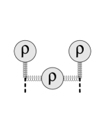
Figure 9: Part of the real contribution to the induced color charge

In principle there is also a contribution from the region with opposite ordering $k_{\perp}^{2}\ll p_{\perp}^{2}$. This component of the induced charge density would contain frequencies which are even smaller than those in $\rho$. However it is exactly canceled by the virtual corrections of Fig.6 as can be checked explicitly from the expression for the BFKL kernel.

So, to reiterate, as we move to lower $x$ we get two distinct contributions. First, there is a Born - Oppenheimer type contribution. It appears because we “renormalize” the notion of staticity by including new (faster) modes in the category of static. This is the $\delta\rho_{faster}$. Physically, this relates to the processes at smaller $x$ that happen at ever faster time scales. Second, there is a new contribution to the charge density which has a long wavelength but also low frequency. This is $\delta\rho_{slower}$. This is not a contribution of the Born - Oppenheimer type and appears since the splitting in terms of the longitudinal momentum does not strictly coincide with the splitting in terms of frequency.

Now, the DLA approximation to DGLAP assumes transverse momentum ordering and therefore includes only $\delta\rho_{faster}$ in the induced charge density. The BFKL evolution on the contrary includes both contributions. Therefore the DLA DGLAP includes in the induced density only contributions which are faster than previously present, and is evolution simultaneously in the longitudinal momentum and frequency. The BFKL evolution includes contributions which at every step in the evolution modify also the slow component of the charge density, and is therefore evolution only in the longitudinal momentum.

The $\delta\rho_{slower}$ contribution to the BFKL kernel is known to be problematic, since it creates a channel through which the nonperturbative small transverse momentum modes couple to the evolution. The result is the infamous random walk in the transverse momentum space [2, 19] in the asymptotic solution of the BFKL equation. Our full nonlinear procedure is similar to the BFKL approach in the sense that it does not discriminate between the field modes on the basis of their frequency. Whether it still suffers from the same low transverse momentum problem is not clear to us at this point. It is possible that the nonlinearities in the equation suppress the low transverse momentum contributions by generating a dynamical scale somewhat like what happens in the finite temperature and finite density equilibrium systems. It would be very interesting to develop a renormalization group procedure in which the evolution parameter is not the longitudinal momentum (like in our approach) and not the transverse momentum (like in the DGLAP evolution) but rather directly the time resolution scale. This kind of approach would consider the contributions of low $k_{\perp}$ modes at low $x$ as part of the initial condition rather than part of the evolution and would thereby provide a cleaner separation of perturbative and nonperturbative effects. A nonlinear evolution obtained in this type of approach should be closely related to the nonlinear evolution equation of Laenen and Levin[20].

Appendix A High and low density situations: the parametric size of $\rho$

The situation that interests us in this paper is the one when the color charge density is high enough so that the nonlinearities are important. Already when looking at the tree graph expansion of a classical field generated by a color charge density $\rho$, we are in a position to judge how big $\rho$ has to be parametrically for all of the terms to contribute equally to the result.

To do this we observe that one may build all diagrams that make up the classical field starting from the linear term

$$\begin{minipage}[c]{28.45274pt} \psfig{width=28.45274pt} \end{minipage}\ {g\rho}$$ (115)

by stripping off a factor $g\rho$ and replacing it successively by either

$$g\ \begin{minipage}[c]{51.21504pt} \psfig{height=51.21504pt} \end{minipage}\begin{minipage}[c]{28.45274pt} ${g\rho}$\\ \vskip 42.67912pt${g\rho}$ \end{minipage}\qquad\mbox{or}\qquad g^{2}\ \begin{minipage}[c]{51.21504pt} \psfig{height=51.21504pt} \end{minipage}{g\rho}\begin{minipage}[c]{28.45274pt} ${g\rho}$\\ \vskip 42.67912pt${g\rho}$ \end{minipage}$$

To generate diagrams which are all of the same order we need to simultaneously satisfy the equations

$$g\cdot{\rm order}(\rho) = g\left(g\cdot{\rm order}(\rho)\right)^{2}$$ (116)

$$g\cdot{\rm order}(\rho) = g^{2}\left(g\cdot{\rm order}(\rho)\right)^{3}$$ (117)

This fixes $1=g^{2}\cdot{\rm order}(\rho)$ i.e. $\rho$ to be of order $g^{-2}$.

It is therefore for $\rho\sim O(g^{-2})$ that the nonlinear effects described by the RG evolution derived in this paper are physically important.

Appendix B Inverting $K$.

In this appendix we invert the operator $K$ which appears in the small fluctuation action

$$K^{ab}_{xy} = -\bigg{[}(\partial^{+})^{2}\delta^{ab}+f^{abc}\rho^{c}\delta(x^{-})\frac{1}{\partial^{-}}\bigg{]}$$ (118)

$$= -\bigg{[}(\partial^{+})^{2}\delta^{ab}-2M^{ab}\delta(x^{-})\bigg{]}$$

First, note that the frequency and the transverse coordinate dependence of $K$ is trivial, and therefore $p^{-}$ and $x_{\perp}$ are conserved quantum numbers in this inversion. For the purpose of this calculation we can imagine that the color matrix $M$ has been diagonalized at every point in $x_{\perp}$ and we will therefore treat it formally as a number.

Let $f^{a}_{\lambda}(x)$ be the set of eigenfunctions of $K$

$$\int dy^{-}K^{ab}(x,y)f^{b}(p^{-},y^{-},x_{\perp})=\lambda f^{a}(p^{-},x^{-},x_{\perp})$$ (119)

Assuming for the moment that the eigenvalues are positive, the eigenfunctions have the form

$$f^{a}_{p^{-},x_{\perp}}(x)=\theta(-x^{-})e^{ip^{+}x^{-}}U^{a}(x_{\perp},p^{-})+\theta(x^{-})\bigg{[}e^{ip^{+}x^{-}}F^{a}(x_{\perp},p^{-})+e^{-ip^{+}x^{-}}G^{a}(x_{\perp},p^{-})\bigg{]}$$ (120)

where $F$ and $G$ are to be determined. Requiring that $f^{a}$ is continuous at $x^{-}=0$ gives $U^{a}=F^{a}+G^{a}$. The first derivative of $f^{a}$ should be discontinuous such that $\partial^{+}$ when acting on it will cancel the $\delta(x^{-})$ in the equation (118). In other words, the discontinuity in the first derivative must be equal to the integral of the delta function across the discontinuity. This gives

$$f^{a}_{cont}=U^{a}_{\alpha}e^{ipx}-i\theta(x^{-})\frac{\sin p^{+}x^{-}}{p^{+}p^{-}}f^{abc}U^{b}_{\alpha}\rho^{c}(x_{\perp}).$$ (121)

These eigenfunctions correspond to a positive eigenvalue

$$\lambda=p^{+2}$$

To determine the proper normalization of the “polarization vector” $U^{a}_{\alpha}$ it is easier to work with the symmetric and anti-symmetric combinations

$$f^{a}_{\alpha sym}=U^{a}_{\alpha}\cos p^{+}x^{-}-i\frac{1}{2p^{+}p^{-}}f^{abc}U^{a}_{\alpha}\rho^{c}\sin p^{+}x^{-}\bigg{[}\theta(x^{-})-\theta(-x^{-})\bigg{]}$$

and

$$f^{a}_{\alpha asym}=iU^{a}_{\alpha}\sin p^{+}x^{-}-i\frac{1}{2p^{+}p^{-}}f^{abc}U^{b}_{\alpha}\rho^{c}\sin p^{+}x^{-}$$

The antisymmetric functions vanish at $x^{-}=0$ and therefore are the same as for $M=0$. Their normalized form is just

$$f^{a}_{\alpha asym}=\sin(p^{+}x^{-})\delta^{a}_{\alpha}$$

The overlap matrix for the symmetric eigenfunctions is

$$\int dx^{-}\bigg{[}f^{a}_{(\alpha,p^{+})}(x)\bigg{]}^{\dagger}\bigg{[}f^{a}_{(\beta,p^{+^{\prime}})}(x)\bigg{]}=\delta(p^{+}-p^{+\prime})\frac{U^{\dagger}U}{2}\bigg{[}1-\frac{(f\cdot\rho)^{2}}{(2p^{+}p^{-})^{2}}\bigg{]}$$

and we get

$$U^{\dagger}U=\frac{2(p^{+})^{2}}{(p^{+})^{2}+M^{2}}$$

These are the eigenfunctions for “continuum” states, the ones corresponding to positive eigenvalues.

Note that since $trf\cdot\rho=0$, the matrix $M$ has both negative and positive eigenvalues. Therefore the eigenvalue equation (119) must also have negative eigenvalues and corresponding “bound state” solutions. The bound state wave function must be symmetric under $x^{-}\rightarrow-x^{-}$ and has the same form as the continuum solution except that $p^{+}$ is imaginary. Requiring that it decay exponentially at large $x^{-}$, we have

$$p^{+}=iM\theta(M)$$

The eigenfunction then is

$$f^{a}_{bs}=NV^{a}_{\alpha}\bigg{[}\theta(x^{-})e^{-Mx^{-}}+\theta(-x^{-})e^{Mx^{-}}\bigg{]}$$ (122)

where $N$ is a normalization factor and $V^{a}_{\alpha}$ are the set of eigenfunctions of $M$ with positive eigenvalue. The normalization factor $N$ is easily calculated and is given by $N^{2}=M$.

It is easily checked that the set of our eigenfunctions is complete. The completeness relation is

$$I\equiv\int\frac{d^{4}p}{(2\pi)^{4}}\bigg{[}a^{a}(x,p)\bigg{]}^{\dagger}\bigg{[}a^{b}(y,p)\bigg{]}=\delta(x-y)\delta^{ab}$$ (123)

This can be written as

$$I=\delta(x_{\perp}-y_{\perp})\int\frac{dp^{-}}{2\pi}I_{1}(x^{-},y^{-},p^{-})$$

where for the continuum solutions we have

$$I_{1} = \theta(x^{-})\theta(y^{-})\bigg{[}\frac{-1}{2}(\mid M\mid+M)\theta(x^{-}+y^{-})e^{-\mid M\mid(x^{-}+y^{-})}$$ (124)

$$- \frac{1}{2}(\mid M\mid-M)\theta(-x^{-}-y^{-})e^{\mid M\mid(x^{-}+y^{-})}$$

$$+ \delta(x^{-}+y^{-})+\int\frac{dp^{+}}{2\pi}2\sin p^{+}x^{-}\sin p^{+}y^{-}\bigg{]}$$

$$+ \theta(x^{-})\theta(-y^{-})\bigg{[}\frac{-1}{2}(\mid M\mid+M)\theta(x^{-}-y^{-})e^{-\mid M\mid(x^{-}-y^{-})}$$

$$- \frac{1}{2}(\mid M\mid-M)\theta(-x^{-}+y^{-})e^{\mid M\mid(x^{-}-y^{-})}+\delta(x^{-}-y^{-})\bigg{]}$$

$$+ (x^{-},y^{-}\rightarrow-x^{-},-y^{-})$$

while for the bound state

$$I_{1} = \frac{1}{2}(\mid M\mid+M)\bigg{[}\theta(x^{-})\theta(y^{-})e^{-\mid M\mid(x^{-}+y^{-})}+\theta(x^{-})\theta(-y^{-})e^{-\mid M\mid(x^{-}-y^{-})}$$ (125)

$$+ (x^{-},y^{-}\rightarrow-x^{-},-y^{-})\bigg{]}$$

All $M$ dependent terms cancel out between the two contributions. Performing the $p^{+}$ integration and adding all the terms establishes the completeness relation (123).

Now that we have the complete set of eigenfunctions, we are ready to invert the operator $K$. But first we should understand the zero modes $p^{+}=0$. These eigenfunctions do not vanish at $x^{-}\rightarrow\pm\infty$ and we should be careful with them, for example when integrating by parts. In fact when calculating the propagator, these eigenfunctions should be excluded entirely from the sum as explained in Section 5. The convenient way to do that is to regulate the factor $1/\lambda$ which enters in the calculation of the propagator as

$$\frac{1}{\lambda}\equiv\frac{\lambda}{\lambda^{2}+\epsilon^{4}}$$

taking the limit $\epsilon\rightarrow 0$ at the end of the calculation. We use the same regulator to regulate a possible singularity $M\rightarrow 0$ in the bound state eigenvalue.

$$\frac{1}{M^{2}}\rightarrow\frac{M^{2}}{M^{4}+\epsilon^{4}}$$

The propagator $K^{-1}$ is calculated as

$$K^{-1}(x^{-},x_{\perp},p^{-},y^{-},y_{\perp},p^{-^{\prime}})=\int d\lambda{1\over\lambda}f_{\lambda,p^{-},x_{\perp}}(x^{-})f^{*}_{\lambda,p^{-},x_{\perp}}(y^{-})\delta(p^{-}-p^{-^{\prime}})\delta(x_{\perp}-y_{\perp})$$ (126)

The result is

$$K^{-1} = \frac{-1}{4i\sqrt{i}\,\epsilon}\Bigg{\{}\theta(x^{-}-y^{-})\bigg{[}e^{i\sqrt{i}\,\epsilon(x^{-}-y^{-})}-ie^{-\sqrt{i}\,\epsilon(x^{-}-y^{-})}\bigg{]}$$ (127)

$$+ M\Bigg{[}\theta(x^{-})\theta(y^{-})\bigg{[}\frac{e^{i\sqrt{i}\,\epsilon(x^{-}+y^{-})}}{M+i\sqrt{i}\,\epsilon}-i\frac{e^{-\sqrt{i}\,\epsilon(x^{-}+y^{-})}}{M-\sqrt{i}\,\epsilon}\bigg{]}$$

$$+ \theta(x^{-})\theta(-y^{-})\bigg{[}\frac{e^{i\sqrt{i}\,\epsilon(x^{-}-y^{-})}}{M+i\sqrt{i}\,\epsilon}-i\frac{e^{-\sqrt{i}\,\epsilon(x^{-}-y^{-})}}{M-\sqrt{i}\,\epsilon}\bigg{]}$$

$$+ (x^{-},y^{-}\rightarrow-x^{-},-y^{-})\Bigg{\}}\delta(p^{-}-p^{-^{\prime}})\delta(x_{\perp}-y_{\perp})$$

Expanding the above expression in powers of $\epsilon$ to order one, we get

$$K^{-1}=\bigg{\{}-{1\over 2}|x^{-}-y^{-}|+{1\over 2}\eta\bigg{[}|x^{-}|+|y^{-}|\bigg{]}-{\eta\over 2M}+{\mu\over 2\sqrt{2}\epsilon}\bigg{\}}\delta(p^{-}-p^{-^{\prime}})\delta(x_{\perp}-y_{\perp})$$ (128)

where we have defined the projection operators $\eta$ and $\mu$ that project on nonzero and zero eigenvalue subspaces of $M$ respectively

$$\mu M=0,\;\;\;\eta M=M$$ (129)

$$\mu+\eta=1,\;\;\mu^{2}=\mu,\;\;\eta^{2}=\eta$$ (130)

Note that the last term in Eq.(128) diverges in the limit $\epsilon\rightarrow 0$. However examining carefully equations in Section 5, we see that $K^{-1}$ always acts on a particular combination of fields $B$ which satisfies the constraint $\mu B=0$ by virtue of the Gauss’ law. We can therefore omit this term from the expression for $K^{-1}$ altogether, which is what we did in the text Eq.(63).

Appendix C Proper normalization of eigenfunctions.

In this appendix we show how to properly normalize eigenfunctions in a theory with a Lagrange multiplier field. Consider a quadratic form

$$S=a_{i}M_{ij}a_{j},\ \ \ \ \ \ \ \ \ i=1,...,N$$ (131)

where the variables $a_{i}$ are constrained by $m$ linear conditions

$$c^{\alpha}_{i}a_{i}=0,\ \ \ \ \ \ \ \alpha=1,...,m$$ (132)

Our problem is to invert $M$ on the subspace whose vectors satisfy Eq.(132). This is the precise analog of the system we deal with in Section 5. Let us assume that all $m$ vectors $c^{\alpha}_{i}$ are linearly independent. In that case they span an $m$ - dimensional subspace $C$ of the original $N$ dimensional vector space $V$. Let $l^{\alpha}$ be an orthonormal basis on this subspace. We can then construct the projection operator

$$P_{ij}=l^{\alpha}_{i}l^{\alpha}_{j}$$ (133)

which projects on $C$.

Then instead of considering the matrix $M$ we should consider

$$\tilde{M}=(1-P)M(1-P)$$ (134)

and invert it on $V-C$. The eigenvalue and eigenfunction equations for this problem are

$$\tilde{M}a=\lambda(1-P)a$$ (135)

or alternatively

$$(1-P)Ma=\lambda a$$

$$c^{\alpha}a=0$$

Clearly the eigenfunctions have to be normalized in the standard way

$$a_{i}^{\lambda}a_{i}^{*\lambda^{\prime}}=\delta_{\lambda,\lambda^{\prime}}$$ (136)

The inverse of $M$ on $V-C$ is constructed as

$$\tilde{M}^{-1}=\sum_{\lambda}{a_{i}^{\lambda}a_{j}^{*\lambda}\over\lambda}$$ (137)

since

$$\tilde{M}\tilde{M}^{-1}=(1-P)M\tilde{M}^{-1}=\sum_{\lambda}a_{i}^{\lambda}a_{j}^{*\lambda}=P_{ij}$$ (138)

An alternative to explicit construction of the projection operator $P$ is introduction of the Lagrange multiplier field, as we did in Section 5. We add to the Lagrangian the term

$$b^{\alpha}c^{\alpha}a$$ (139)

The eigenvalue equations we have to solve now are

$$Ma+b^{\alpha}c^{\alpha}=\lambda a$$

$$c^{\alpha}a=o$$

Now since, $Pc^{\alpha}=c^{\alpha}$ and $Pa=0$, this equation gives

$$PMa+b^{\alpha}c^{\alpha}=0$$ (140)

Solving this for $b^{\alpha}$ and substituting back into Eq.(C) we obtain again Eq.(C). This proves that the eigenfunctions obtained through introduction of the Lagrange multiplier are the same as in the straightforward calculation in which the constraint is solved explicitly through construction of $P$. It is clear then that the normalization of these functions should be the standard normalization Eq.(136).

Appendix D The BFKL limit of the general evolution equation.

In this section we will show in some detail how our general expressions for $\chi^{ab}$ and $\sigma^{a}$ give the BFKL kernel. To do so, we have to take the limit of small $\rho$ in the evolution equation Eq.(51). In fact it is more convenient to consider directly the equation for the density correlation function Eq.(54). As was shown in [12], using Eqs.(27) and (4) the unintegrated gluon density $\phi(k_{\perp})$ (which is the quantity which evolves according to the BFKL equation) to leading order in $\rho$ is just the charge density two point function $<\rho(k_{\perp})\rho(-k_{\perp})>$. The BFKL equation should therefore be just the weak field limit of Eq.(54).

To verify this we will need the expressions for $\chi^{ab}$ and $\sigma^{a}$ expended to first order in $\rho$. Let us consider the contributions of the real diagrams given by $\delta\rho_{real}$ in equation (refeq:totalrhoreal). Using the expressions for $v_{+}^{i}$ and $\gamma_{+}$ and $1/D^{2}$ expanded to first order in $\alpha$

$$\gamma^{i}_{+} = 2{\partial^{i}\over\partial^{2}_{\perp}}\bigg{[}\alpha v_{-}+(\partial\alpha){\partial v_{-}\over\partial^{2}_{\perp}}\bigg{]}$$

$$v^{i}_{+} = 2\alpha^{i}{\partial v_{-}\over\partial^{2}_{\perp}}+v^{i}_{-}-2{\partial^{i}\over\partial^{2}_{\perp}}\bigg{[}\alpha v_{-}+(\partial\alpha){\partial v_{-}\over\partial^{2}_{\perp}}\bigg{]}$$

$${1\over D^{2}_{\perp}} = {1\over\partial^{2}_{\perp}}-{1\over\partial^{2}_{\perp}}(\partial\alpha+\alpha\partial){1\over\partial^{2}_{\perp}}$$ (141)

leads to

$$\delta\rho^{a}_{1}(x_{\perp})=-2f^{abc}\bigg{[}\alpha^{b}v^{c}_{-}-\rho^{b}{\partial v^{c}_{-}\over\partial^{2}_{t}}\bigg{]}$$ (142)

In the momentum space representation

$${\partial^{i}\over\partial^{2}_{t}}v^{i}_{-}=i\int{d^{2}p_{\perp}\over(2\pi)^{2}}d^{2}y_{\perp}{p^{i}\over p^{2}_{\perp}}e^{ip_{\perp}(x_{\perp}-y_{\perp})}v^{i}_{-}(y_{\perp})$$ (143)

With these expressions we have

$$\delta\rho^{a}_{1}(x_{\perp})\delta\rho^{b}_{1}(y_{\perp})=4g^{2}f^{acd}f^{bef}\bigg{[}\alpha^{c}v^{d}_{-}-\rho^{c}{\partial v^{d}_{-}\over\partial^{2}_{\perp}}\bigg{]}_{x_{\perp}}\bigg{[}\alpha^{e}v^{f}_{-}-\rho^{e}{\partial v^{f}_{-}\over\partial^{2}_{\perp}}\bigg{]}_{y_{\perp}}$$ (144)

To this order the normalization of $v^{i}_{i}$ is

$$<v^{id}_{-}(x_{\perp})v^{\ast jf}_{-}(y_{\perp})>=\delta^{ij}\delta^{df}\delta^{2}(x_{\perp}-y_{\perp}){1\over 2\pi}{1\over 2}$$ (145)

We then have

$$<\delta\rho^{a}_{1}(x_{\perp})\delta\rho^{b}_{1}(y_{\perp})>=g^{2}f^{acd}f^{bed}{1\over\pi}\ln 1/x\bigg{\{}\alpha^{c}(x_{\perp})\alpha^{e}(y_{\perp})\delta^{2}(x_{\perp}-y_{\perp})$$ (146)

$$+ i\bigg{[}\alpha^{ic}(x_{\perp})\rho^{e}(y_{\perp})-\rho^{c}(x_{\perp})\alpha^{ie}(y_{\perp})\bigg{]}\int{d^{2}p_{\perp}\over(2\pi)^{2}}{p^{i}\over p^{2}_{\perp}}e^{ip_{\perp}(x_{\perp}-y_{\perp})}$$

$$+ \rho^{c}(x_{\perp})\rho^{e}(y_{\perp})\int{d^{2}p_{\perp}\over(2\pi)^{2}}{1\over p^{2}_{\perp}}e^{ip_{\perp}(x_{\perp}-y_{\perp})}\bigg{\}}$$

This expression coincides with Eqns.(53,54,55) in [12]. Using $\alpha^{i}=-{\partial^{i}\rho\over\partial^{2}}$ we obtain

$$\delta\rho^{a}_{1}(k_{\perp})\delta\rho^{a}_{1}(-k_{\perp}) = {{2g^{2}N_{c}}\over{(2\pi)^{3}}}\int d^{2}p_{\perp}\rho^{a}(p_{\perp})\rho^{a}(-p_{\perp}){{k_{\perp}^{2}}\over{p_{\perp}^{2}(p_{\perp}-k_{\perp})^{2}}}$$ (147)

This is precisely the real part of the BFKL kernel.

It is straightforward to repeat the above procedure for the contribution of virtual diagrams $<\delta\rho^{a}_{2}(x_{\perp})>$ (5.3). In this case, the term $R^{ab}$ vanishes to order $\alpha$. Using our expanded expressions for $a_{+}$ and $\gamma_{+}$ and noticing that $\gamma_{+}$ starts at order $\alpha$, the first line in (5.3) gives

$$<\delta\rho^{a}_{2}(x_{\perp})>_{(1)}\!=\!-{g^{2}\over 2\pi}f^{dbc}f^{abc}\int\!d^{2}y_{\perp}\rho^{d}(y_{\perp})\int\!{d^{2}p_{\perp}\over(2\pi)^{2}}{d^{2}q_{\perp}\over(2\pi)^{2}}{p_{\perp}\cdot q_{\perp}\over p^{2}_{\perp}q^{2}_{\perp}}e^{i(p_{\perp}+q_{\perp})(x_{\perp}-y_{\perp})}$$ (148)

This agrees with the corresponding term in [12]. In the second line in the expression for $\delta\rho^{a}_{2}$ (5.3), we can take the order $\alpha^{0}$ inside the brackets since there is already an explicit factor of $\rho$ present. This gives

$$<\delta\rho^{a}_{2}(x_{\perp})>_{(2)}=-{g^{2}N_{c}\over(2\pi)^{3}}\ln 1/x\rho^{a}(x_{\perp})\int{d^{2}p_{\perp}\over p^{2}_{\perp}}$$ (149)

which is exactly equation (50) in [12]. Collecting all the contributions, substituting them into Eq.(54) and identifying the density correlator with the unintegrated gluon density $\phi$ we obtain

$${d\over d\ln{1\over x}}\phi(k_{\perp})=-{{g^{2}N_{c}}\over{(2\pi)^{3}}}\int d^{2}p_{\perp}{{k_{\perp}^{2}}\over{p_{\perp}^{2}(p_{\perp}-k_{\perp})^{2}}}\Bigg{[}\phi(k_{\perp})-2\phi(p_{\perp})\Bigg{]}$$ (150)

This is precisely the BFKL equation [2].

Acknowledgements We are grateful to Larry McLerran for numerous discussions on a variety of topics related to the subject of this paper. We have also benefited from interesting discussions with A. Leonidov, E. Levin, A. White and M. Wüsthoff. The work of J.J.M. was supported by DOE contract DOE-Nuclear DE-FG02-87ER-40328. A.K. was supported by DOE contract DOE High Energy DE-AC02-83ER40105 and the PPARC Advanced Fellowship. HW was supported by the EC Program “Training and Mobility of Researchers”, Network “Hadronic Physics with High Energy Electromagnetic Probes”, contract ERB FMRX-CT96-0008.

References

• [1] H1 Collaboration, I. Abe et al., Nucl. Phys. B407 (1993), 515; T. Ahmed et al., Nucl. Phys. B439 (1995), 471; ZEUS Collaboration, M. Derrick et al., Phys. Lett. B316 (1993), 412; Z. Phys. C65 (1995), 379.
• [2] E.A. Kuraev, L.N. Lipatov and V.S. Fadin, Sov. Phys. JETP 45 (1977), 199; Ya.Ya. Balitsky and L.N. Lipatov, Sov. J. Nucl. Phys. 28 (1978), 22.
• [3] A.D. Martin, W.J. Stirling and R.G. Roberts Phys.Rev. D50, 6734 (1994); CTEQ collaboration, H.L. Lai et. al. Phys.Rev. D51, 4763 (1995).
• [4] L.V. Gribov, E.M. Levin and M.G. Ryskin, Phys. Rep 100 (1981).
• [5] A. L. Ayala, M. B. Gay Ducati and E. M. Levin Nucl.Phys. B493 305 (1997);
• [6] Y. V. Kovchegov, A. H. Mueller and S. Wallon, Unitarity Corrections and High Field Strengths in High Energy Hard Collisions, hep-ph/9704369
• [7] A.H. Mueller and J.W. Qiu, Nucl. Phys. B268 (1986), 427.
• [8] L.N. Lipatov, ”Small-x Physics in Perturbative QCD”, hep-ph/9610276.
• [9] J. Bartels, Nucl. Phys. B175 (1980) 365; J. Kwiecinski and M. Praszalowicz Phys. Lett. 94B (1980) 413; G.P. Korchemsky, Nucl. Phys. B462, (1996) 333.
• [10] A. Mueller, Nucl. Phys. B437 (1995), 107.
• [11] J. Jalilian-Marian, A. Kovner, L. McLerran and H. Weigert, Phys.Rev. D55, 5414 (1997)
• [12] J. Jalilian-Marian, A. Kovner, A. Leonidov and H. Weigert, hep-ph/9701284, to be published in Nucl. Phys. B;
• [13] J. Jalilian-Marian, A. Kovner, A. Leonidov and H. Weigert, hep-ph/9706377;
• [14] L. McLerran and R. Venugopalan, Phys. Rev. D49 (1994), 2233;  D49 (1994), 3352.
• [15] V.S. Fadin and L.N. Lipatov, Nucl.Phys.B477, 767 (1996); V.S. Fadin, M.I. Kotskii, L.N. Lipatov hep-ph/9704267;
• [16] A. Ayala, J. Jalilian-Marian, L. McLerran and R. Venugopalan, Phys. Rev.D52 (1995), 2935; Phys. Rev.D53 (1996), 458.
• [17] A. Kovner, L. McLerran and H. Weigert, Phys. Rev. D52, 3809 (1995); Phys. Rev. D52, 6231 (1995); Y. V. Kovchegov and D. H. Rischke, hep-ph/9704201 ; M. Gyulassy and L. McLerran, nucl-th/9704034
• [18] A.Krasnitz and R. Venugopalan, hep-ph/9706329
• [19] A.J. Askew, J. Kwiecinski, A.D. Martin and P.J. Sutton Phys.Rev. D49 (1994), 4402;
• [20] E. Laenen and E. Levin, Nucl. Phys. B451 (1995), 297.