CERN-TH/97-235

RAL-TR-97-044

NORDITA-97/62 P

TUM/T39-97-21

hep-ph/9709376

Inelastic photoproduction of polarised $J/\psi$
M. Beneke Theory Division, CERN, CH-1211 Geneva 23
M. Krämer Rutherford Appleton Laboratory
Chilton, Didcot, OX11 0QX, England
M. Vänttinen NORDITA, Blegdamsvej 17, DK-2100 Copenhagen Ø

The comparison of $J/\psi$ photoproduction data in the inelastic region with theoretical predictions based on the NRQCD approach has remained somewhat ambiguous and controversial, in particular at large values of the inelasticity variable $z$. We study the polar and azimuthal decay angular distribution of $J/\psi$ mesons as functions of $z$ and transverse momentum $p_{t}$. Future measurements of decay angular distributions at the HERA $ep$ collider will provide a new test of theoretical approaches to factorisation between perturbation theory and quarkonium bound-state dynamics and shed light on the colour-octet production fraction in various regions of $z$ and $p_{t}$.

1 Introduction

The production of quarkonium in various processes, especially at high-energy colliders (for reviews, see [1, 2]), has been the subject of considerable interest during the past few years. New data have been taken at $p\bar{p}$, $ep$ and $e^{+}e^{-}$ colliders, and a wealth of fixed-target data also exist. In theory, progress on factorisation between perturbative and the quarkonium bound state dynamics has been made. The earlier ‘colour-singlet model’ has been superseded by a consistent and rigorous approach, based on non-relativistic QCD (NRQCD) [3], an effective field theory that includes the so-called colour-octet mechanisms. On the other hand, the ‘colour evaporation’ model of the early days of quarkonium physics [4] has been revived [5]. Despite these developments the range of applicability of these approaches to the practical case of charmonium is still subject to debate, as is the quantitative verification of factorisation. The problematic aspect is that, because the charmonium mass is still not very large with respect to the QCD scale, non-factorisable corrections may not be suppressed enough, if the quarkonium is not part of an isolated jet, and the expansions in NRQCD may not converge very well. In this situation cross checks between various processes, and predictions of observables such as quarkonium polarisation and differential cross sections, are crucial in order to assess the importance of different quarkonium production mechanisms, as well as the limitations of a particular theoretical approach. In this paper we discuss how polar and azimuthal decay angular distributions of $J/\psi$, produced by real photons colliding on a proton target in the inelastic region $p_{t}>1\,$GeV (or, more conventionally, $z\equiv p_{\psi}\cdot p_{p}/p_{\gamma}\cdot p_{p}<0.9$), may serve this purpose.

In the NRQCD approach, to which we adhere in this paper, the cross section for producing a charmonium state $H$ in a photon–proton collision is written as a sum of factorisable terms,

$$d\sigma(H)=\sum_{i,j\in\{q,g,\gamma\}}\int dx_{1}dx_{2}\,f_{i/\gamma}(x_{1})f_{j/p}(x_{2})\,\sum_{n}d\hat{\sigma}(i+j\to c\bar{c}[n])\,\langle{\cal O}_{n}^{H}\rangle,$$ (1)

where $n$ denotes the colour, spin and angular momentum state of an intermediate $c\bar{c}$ pair and $f_{i/\gamma}$ and $f_{j/p}$ the parton distributions in the photon and the proton, respectively. The short-distance cross sections $d\hat{\sigma}(i+j\to c\bar{c}[n])$ can be calculated perturbatively in the strong coupling $\alpha_{s}$. The matrix elements $\langle{\cal O}_{n}^{H}\rangle\equiv\langle 0|{\cal O}_{n}^{H}|0\rangle$ (see [3] for their definition) are related to the non-perturbative transition probabilities from the $c\bar{c}$ state $n$ into the quarkonium $H$. The magnitude of these probabilities is determined by the intrinsic velocity $v$ of the bound state. Thus the above sum is a double expansion in $\alpha_{s}$ and $v$.

Within NRQCD the leading term in $v$ to inelastic photoproduction of $J/\psi$ comes from an intermediate $c\bar{c}$ pair in a colour-singlet ${}^{3}\!S_{1}$ state and coincides with the colour-singlet model result. (The notation for the angular momentum configuration is ${}^{2S+1}\!L_{J}$ with $S$, $L$ and $J$ denoting spin, orbital and total angular momentum, respectively.) Cross sections [6], polar [7], and polar and azimuthal [8] decay angular distributions have been calculated for the direct-photon contribution, in which case $i=\gamma$ and $f_{\gamma/\gamma}(x)=\delta(1-x)$ in (1). The angular integrated cross section is known to next-to-leading order (NLO) in $\alpha_{s}$ [9]. The colour-singlet contribution, including next-to-leading corrections in $\alpha_{s}$, is known to reproduce the unpolarised data adequately. But there is still a considerable amount of uncertainty in the normalisation of the theoretical prediction, which arises from the value of the charm quark mass and the wave-function at the origin, as well as the choice of parton distribution functions and renormalisation/factorisation scale.

At order $v^{4}\sim 0.05$–$0.1$ relative to the colour-singlet contribution, the $J/\psi$ can also be produced through intermediate colour-octet ${}^{3}\!S_{1}$, ${}^{1}\!S_{0}$ and ${}^{3}\!P_{J}$ configurations. In the inelastic region, they have been considered in [10, 11] for the direct photon contribution and in [12] for resolved photons, in which case the photon participates in the hard scattering through its parton content. Colour-octet contributions to the total photoproduction cross section (integrated over all $z$ and $p_{t}$) are known to next-to-leading order [13]. The polarisation of inelastically produced $J/\psi$ due to these additional production mechanisms, however, has not been calculated so far.

Because the colour-octet contributions are suppressed as $v^{4}$, but, in the inelastic region, contribute at the same order in $\alpha_{s}$ as the colour-singlet contribution, they are of interest only if they are enhanced by other factors, either numerical or kinematical. In this respect the situation is similar to a certain $v^{2}$-correction, which arises already in the colour-singlet model [14] and becomes kinematically enhanced at $z$ close to 1. The colour-octet production channels are indeed kinematically different from the colour-singlet one, because the ${}^{1}\!S_{0}$ and ${}^{3}\!P_{J}$ configurations can be produced through $t$-channel exchange of a gluon already at lowest order in $\alpha_{s}$. (For the ${}^{3}\!S_{1}$ octet this is true for the resolved process.) This leads to a significantly enhanced amplitude, in particular in the large-$z$ region. The colour-octet contributions to $J/\psi$ photoproduction are indeed strongly peaked at large $z$ [10, 11]. Such a shape is not supported by the data, which at first sight could lead to a rather stringent constraint on the octet matrix elements $\langle{\cal O}_{8}[n]\rangle$, $n\in\{^{1}\!S_{0},^{3}\!P_{0}\}$ and to an inconsistency with the values obtained for these matrix elements from other processes. However, the peaked shape of the $z$-distribution is derived neglecting the energy transfer in the non-perturbative transition $c\bar{c}[n]\to J/\psi+X$. In reality the peak may be considerably smeared [15] as a consequence of resumming kinematically enhanced higher-order corrections in $v^{2}$ and no constraint or inconsistency can be derived from the endpoint behaviour of the $z$-distribution at present. As a consequence, the role of octet contributions to the direct process remains unclear. The resolved photon contribution, on the other hand, could be entirely colour-octet dominated [12, 16]. The $z$-distribution should then begin to rise again at small $z$, if the colour-octet matrix elements are as large as suggested by NRQCD velocity scaling rules [17, 3] and fits to hadroproduction data.

Our motivation for considering the decay angular distributions, including all direct and resolved production mechanisms, is to provide another observable that can clarify the relative importance of colour-octet production in photoproduction in different kinematic regions. Many of the above-mentioned uncertainties and difficulties do not affect the polarisation yield. For example, the resummation that is necessary in the endpoint region may lead to a significant redistribution of $d\sigma/dz$ in $z$, but affects the normalised decay angular distributions to a lesser degree, if they do not have a strong $z$-dependence in the region affected by the smearing. We find that some angular coefficients, especially those for the azimuthal angle dependence, take essentially different values in the colour-singlet and colour-octet processes. A measurement of decay angular distributions would therefore provide information on the relevance of colour-octet production, also at $z$ close to 1, which is largely independent of normalisation uncertainties.

The polarisation of the $J/\psi$ can be determined by measuring the angular distribution of the leptonic decay $J/\psi\rightarrow l^{+}l^{-}$. To date, experimental measurements of $J/\psi$ polarisation exist only for diffractive (elastic and proton dissociation) photoproduction [18, 19], to which the inclusive formalism of NRQCD does not apply, and for fixed-target hadroproduction [20]. The latter can be compared with predictions obtained in the colour-singlet model [21] and NRQCD [22, 23] for $p_{t}$-integrated cross sections. As discussed in [2] the experimental finding of no polarisation is only marginally consistent with the NRQCD prediction. Photoproduction offers another opportunity to learn about whether the $J/\psi$ polarisation carries information on the spin of the heavy quark pair produced at short distances, which is expected in theoretical approaches in which spin symmetry is at work. With the expected increase in luminosity at the HERA $ep$ collider, polarisation in photoproduction of $J/\psi$ at different values of $z$ and $p_{t}$ could provide an attractive diagnostic tool in addition to the widely discussed polarisation measurement in $p\bar{p}$ collisions at the Fermilab Tevatron [?–?].

The paper is organised as follows: Section 2 discusses the production mechanisms and calculational details regarding decay angular distributions. In Section 3 we pause for theoretical considerations that influence our choice of cuts and other parameters in the analysis. Section 4 presents results and their discussion, followed by a summary in Section 5. Appendix A contains the covariant definitions of coordinate systems and polarisation vectors and Appendix B summarises the density matrices for all subprocesses considered in the paper.

2 Production mechanisms and cross sections

We assume that the $J/\psi$ transverse momentum $p_{t}>1\,$GeV, in order to suppress the diffractive contribution and higher-twist corrections in general. Away from $p_{t}=0$ (or $z=1$) the leading-twist hard subprocesses contributing to inelastic $J/\psi$ production can be classified as follows:

1. Direct photon mechanisms. At leading order in the strong coupling constant, $O(\alpha\alpha_{s}^{2})$, these are

   $$\gamma+g \rightarrow c\bar{c}\left[{}^{3}\!S_{1}^{(1)},\,^{3}\!S_{1}^{(8)},\,^{1}\!S_{0}^{(8)},\,^{3}\!P_{J}^{(8)}\right]+g,$$ (2)

   $$\gamma+q/\bar{q} \rightarrow c\bar{c}\left[{}^{3}\!S_{1}^{(8)},\,^{1}\!S_{0}^{(8)},\,^{3}\!P_{J}^{(8)}\right]+q/\bar{q},$$ (3)

   where the initial-state parton originates from the target proton.

2. Resolved photon mechanisms. At leading order, $O(\alpha_{s}^{3})$, the subprocesses are

   $$g+g \rightarrow c\bar{c}\left[{}^{3}\!S_{1}^{(1)},\,^{3}\!S_{1}^{(8)},\,^{1}\!S_{0}^{(8)},\,^{3}\!P_{J}^{(8)}\right]+g,$$ (4)

   $$g+q/\bar{q} \rightarrow c\bar{c}\left[{}^{3}\!S_{1}^{(8)},\,^{1}\!S_{0}^{(8)},\,^{3}\!P_{J}^{(8)}\right]+q/\bar{q},$$ (5)

   $$q+\bar{q} \rightarrow c\bar{c}\left[{}^{3}\!S_{1}^{(8)},\,^{1}\!S_{0}^{(8)},\,^{3}\!P_{J}^{(8)}\right]+g,$$ (6)

   where one of the initial-state partons originates from the photon and the other originates from the proton.

The direct-photon mechanisms dominate in the region $z\;\hbox to0.0pt{\lower 3.5pt\hbox{$\mathchar 0\relax\sim$}\hss}\raise 1.0pt\hbox{$>$}\;0.2$, whereas resolved-photon mechanisms become important in the region $z\;\hbox to0.0pt{\lower 3.5pt\hbox{$\mathchar 0\relax\sim$}\hss}\raise 1.0pt\hbox{$<$}\;0.2$. (These numbers depend on the values of the colour-octet matrix elements, as well as on the $p_{t}$-cut.) At HERA energies, photon–quark fusion can contribute about 10%–15% to the cross section at large $z$. Quark–gluon fusion constitutes about 20%–40% of the resolved cross section at $z\;\hbox to0.0pt{\lower 3.5pt\hbox{$\mathchar 0\relax\sim$}\hss}\raise 1.0pt\hbox{$<$}\;0.2$ and becomes more important than gluon–gluon fusion at larger $z$. Quark–antiquark fusion is always completely negligible.

The above list includes those colour-octet production channels that are suppressed by at most $v^{4}$ relative to the leading colour singlet production channel. The suppression of the octet contributions follows from a multipole expansion of the non-perturbative transition $c\bar{c}[n]\to J/\psi+X$. From a ${}^{3}\!P_{J}^{(8)}$ intermediate state, the physical $J/\psi$ state can be reached by a single chromoelectric dipole transition, from a ${}^{3}\!S_{1}^{(8)}$ state by two consecutive electric dipole transitions, and from a ${}^{1}\!S_{0}^{(8)}$ state by a chromomagnetic dipole transition. Each electric dipole transition brings a factor $v^{2}$, and the magnetic dipole transition a factor $v^{4}$. In addition, the hard production vertex for a $P$-wave $c\bar{c}$ state is suppressed already by $v^{2}$ relative to production in an $S$-wave state. In photon-gluon fusion, the ${}^{3}\!S_{1}^{(8)}$-amplitude is kinematically identical to the ${}^{3}\!S_{1}^{(1)}$-amplitude. The ${}^{3}\!S_{1}^{(8)}$-channel is therefore insignificant for the direct-photon contribution.

In resolved photon interactions, on the other hand, the ${}^{3}\!S_{1}^{(8)}$-channel dominates at $p_{t}\;\hbox to0.0pt{\lower 3.5pt\hbox{$\mathchar 0\relax\sim$}\hss}\raise 1.0pt\hbox{$>$}\;5\,$GeV, because it includes a gluon fragmentation component [28], in both the gluon–gluon and gluon–quark fusion contributions, and therefore falls only as $1/p_{t}^{4}$ at large $p_{t}$. The resolved photon amplitudes are identical to those relevant to $J/\psi$ production in hadron–hadron collisions [29, 26] and at HERA energies the relative importance of the various contributions as functions of $p_{t}$ is nearly the same as at Tevatron energies.

The direct-photon mechanisms above all decrease at least as $1/p_{t}^{6}$ at large $p_{t}$, with the exception of $\gamma+q\to c\bar{c}[^{3}\!S_{1}^{(8)}]+q$. Fragmentation contributions in photon-gluon fusion exist only at the next order in $\alpha_{s}$. They exceed the leading-order contributions at $p_{t}\;\hbox to0.0pt{\lower 3.5pt\hbox{$\mathchar 0\relax\sim$}\hss}\raise 1.0pt\hbox{$>$}\;10\,$GeV [30, 16]. We therefore conclude that our list includes all important leading-twist production mechanisms for all $z$ and as long as $p_{t}\;\hbox to0.0pt{\lower 3.5pt\hbox{$\mathchar 0\relax\sim$}\hss}\raise 1.0pt\hbox{$<$}\;10\,$GeV.

We expect that higher-twist corrections due to multiple interactions with the proton or photon remnant would be suppressed as a power of $\Lambda^{2}/(Q^{2}+p_{t}^{2})$, where $\Lambda\;\hbox to0.0pt{\lower 3.5pt\hbox{$\mathchar 0\relax\sim$}\hss}\raise 1.0pt\hbox{$<$}\;1\,$GeV is a typical QCD scale and $Q$ is one of the scales involved in the bound state dynamics, $Q\approx m_{c},m_{c}v$, or $m_{c}v^{2}$. Since $mv^{2}\sim\Lambda$ for charmonium and bottomonium, one may expect large higher-twist corrections at small $p_{t}$, when the heavy quark–antiquark pair moves parallel with a remnant jet and remains in its hadronization region over a time $1/\Lambda$ in the quarkonium rest frame.

The differential cross section for $J/\psi$ production and its subsequent leptonic decay $J/\psi\to l^{+}l^{-}$ through any of the resolved-photon subprocesses can be written as

$$\frac{1}{B_{ll}}\,\frac{d\sigma^{ij}}{d\Omega dzdp_{t}} = \int\limits_{x_{1,min}}^{1}\!dx_{1}\,f_{i/\gamma}(x_{1},\mu_{F})f_{j/p}(x_{2},\mu_{F})\,\frac{1}{16\pi\hat{s}^{2}}\,\frac{2x_{1}x_{2}p_{t}}{z(x_{1}-z)}$$

$$\times\frac{3}{8\pi}\left[\,\rho^{ij}_{11}+\rho^{ij}_{00}+(\rho^{ij}_{11}-\rho^{ij}_{00})\cos^{2}\theta+\sqrt{2}\,{\rm Re}(\rho^{ij}_{10})\sin 2\theta\cos\phi+\rho^{ij}_{1,-1}\sin^{2}\theta\cos 2\phi\,\right],$$

where $B_{ll}$ is the $J/\psi\to l^{+}l^{-}$ branching ratio, $s=(p_{\gamma}+p_{p})^{2}$, $\hat{s}=x_{1}x_{2}s$ and the parton distribution of the proton is evaluated at

$$x_{2}=\frac{x_{1}p_{t}^{2}+M^{2}(x_{1}-z)}{sz(x_{1}-z)}$$ (8)

with factorisation scale $\mu_{F}$. Here and in the following we use $M=2m_{c}$. The variables $z$ and $p_{t}$ are subject to the restriction

$$(1-z)(sz-M^{2})>p_{t}^{2}$$ (9)

and

$$x_{1}>x_{1,min}=\frac{z(sz-M^{2})}{sz-p_{t}^{2}-M^{2}}.$$ (10)

The angles $\theta$ and $\phi$ refer to the polar and azimuthal angle of the $l^{+}$ in the $J/\psi$ decay with respect to a coordinate system defined in the $J/\psi$ rest frame. (See Appendix A for details on their definition.) Finally

$$\rho^{ij}_{\lambda\lambda^{\prime}}\equiv A[ij\rightarrow J/\psi(\lambda)+X]\,A^{*}[ij\rightarrow J/\psi(\lambda^{\prime})+X]$$ (11)

are density matrix elements for $J/\psi$ production, where a summation (average) over the spins of $X$ ($i,j$) is understood. The kinematical relations for the direct-photon process follow from setting $i=\gamma$ and $f_{\gamma/\gamma}(x_{1},\mu_{F})=\delta(1-x_{1})$.

The polarisation analysis in NRQCD [25, 23, 32] is based on the symmetries of the NRQCD Lagrangian, of which spin and rotational symmetry are crucial. In electric dipole transitions the heavy quark spins remain intact, so that the $J/\psi$ spin orientation will be the same as the perturbatively calculable orientation of the total $c\bar{c}$ spin ${\bf s}_{q}+{\bf s}_{\bar{q}}$ in the intermediate state. The ${}^{1}\!S_{0}^{(8)}$ intermediate state is rotationally invariant and leads to random orientation of the $J/\psi$ spin. Technically, we have

$$\rho^{ij}_{\lambda\lambda^{\prime}}=\rho^{ij}_{\lambda\lambda^{\prime}}[^{3}\!S_{1}^{(1)}]+\rho^{ij}_{\lambda\lambda^{\prime}}[^{3}\!S_{1}^{(8)}]+\rho^{ij}_{\lambda\lambda^{\prime}}[^{1}\!S_{0}^{(8)}]+\rho^{ij}_{\lambda\lambda^{\prime}}[\{S=1,L=1\}^{(8)}]+\ldots,$$ (12)

where $\rho^{ij}_{\lambda\lambda^{\prime}}[n]$ refers to production through a $c\bar{c}$ pair in a state $n$. The above decomposition implies that no interference occurs between the amplitudes for the different terms in the sum. The symmetries of NRQCD do not forbid interference of different ${}^{3}\!P_{J}$-states. One finds [25]

$$\rho^{ij}_{\lambda\lambda^{\prime}}[\{S=1,L=1\}^{(8)}] \propto \sum_{L_{z}}A[ij\to c\bar{c}[(1L_{z};1\lambda)]+X]\,A^{*}[ij\to c\bar{c}[(1L_{z};1\lambda^{\prime})]+X]$$ (13)

$$\not=\,\sum_{J=0,1,2}\rho^{ij}_{\lambda\lambda^{\prime}}[^{3}\!P_{J}^{(8)}],$$

where the quantum numbers of the $c\bar{c}$ pair refer to $(LL_{z},SS_{z})$. NRQCD factorisation implies that the density matrices can be written as

$$\rho^{ij}_{\lambda\lambda^{\prime}}[n]=K^{ij}[n]_{ab\ldots}\,\langle{\cal O}^{J/\psi}_{\lambda\lambda^{\prime}}[n]_{ab\ldots}\rangle,$$ (14)

where $\langle{\cal O}^{J/\psi}_{\lambda\lambda^{\prime}}[n]_{ab\ldots}\rangle$ is a NRQCD matrix element with Cartesian indices $a,b,\ldots$, and $K^{ij}[n]_{ab\ldots}$ the corresponding short-distance coefficient. The final step is a tensor decomposition of these matrix elements, which, in the case of interest, can be formulated as a projection of the $c\bar{c}$ production amplitude. For $J/\psi$ production at the considered order in $v^{2}$, the symmetries of NRQCD are sufficient to reduce all non-perturbative input to the four parameters $\langle{\cal O}^{J/\psi}[n]\rangle$ with $n\in\{^{3}\!S_{1}^{(1)},^{3}\!S_{1}^{(8)},^{1}\!S_{0}^{(8)},^{3}\!P_{0}^{(8)}\}$ defined as for unpolarised $J/\psi$ production.

The calculation then consists of evaluating the density matrix elements for each separate term in (12) and all partonic subprocesses. We express these matrices as

$$\rho_{\lambda\lambda^{\prime}}^{ij}[n] = A^{ij}[n]\,[\epsilon^{*}(\lambda)\cdot\epsilon(\lambda^{\prime})]$$ (15)

$$\mbox{}+M^{2}B^{ij}[n]\,[p_{1}\cdot\epsilon^{*}(\lambda)\;p_{1}\cdot\epsilon(\lambda^{\prime})]+M^{2}C^{ij}[n]\,[p_{2}\cdot\epsilon^{*}(\lambda)\;p_{2}\cdot\epsilon(\lambda^{\prime})]$$

$$\mbox{}+M^{2}D^{ij}[n]\,[p_{1}\cdot\epsilon^{*}(\lambda)\;p_{2}\cdot\epsilon(\lambda^{\prime})+p_{2}\cdot\epsilon^{*}(\lambda)\;p_{1}\cdot\epsilon(\lambda^{\prime})],$$

where $\epsilon(\lambda)$ is the $J/\psi$ polarisation vector, $p_{1}$ is the momentum of the photon (or the parton originating from the photon in resolved contributions), and $p_{2}$ is the momentum of the parton in the target. The coefficients $A,B,C,D$ are independent of the choice of axes in the $J/\psi$ rest frame and proportional to a NRQCD matrix element. Their analytic expressions are collected in Appendix B.

The decay angular distribution in the $J/\psi$ rest frame is often parametrised as

$$\frac{d\sigma}{d\Omega dy}\propto 1+\lambda(y)\cos^{2}\theta+\mu(y)\sin 2\theta\cos\phi+\frac{\nu(y)}{2}\sin^{2}\theta\cos 2\phi,\vspace*{0.2cm}$$ (16)

where $y$ stands for a set of variables and $\lambda,\mu,\nu$ are obviously related to (appropriate integrals of) the density matrix elements as

$$\lambda=\frac{\rho_{11}-\rho_{00}}{\rho_{11}+\rho_{00}},\qquad\mu=\frac{\sqrt{2}\,{\rm Re}\,\rho_{10}}{\rho_{11}+\rho_{00}},\qquad\nu=\frac{2\rho_{1,-1}}{\rho_{11}+\rho_{00}}.\vspace*{0.2cm}$$ (17)

Because of the dependence of $\epsilon(\lambda)$ on the definition of a coordinate system (see Appendix A), the parameters $\lambda,\mu,\nu$ depend on this definition.

3 Theoretical considerations

In this Section we discuss some theoretical issues that influence our choice of cuts. We also motivate the values of NRQCD long-distance matrix elements that we subsequently use.

The NRQCD expansion of the quarkonium production cross section applies to the leading-twist contribution of an inclusive production cross section. Leading-twist means that the result is accurate up to corrections that scale as some power of $\Lambda/m_{c}$ in the limit that $m_{c}\to\infty$. Up to such corrections, NRQCD also applies to the total $J/\psi$ photoproduction cross section. The leading contribution is $O(\alpha\alpha_{s})$ and purely colour-octet [10, 33]. It formally contributes only at $z=1$, $p_{t}=0$, i.e. in the diffractive region. Soft-gluon emission during conversion of the colour-octet $c\bar{c}$ pair into a $J/\psi$ is expected to ‘smear’ the delta-functions at $z=1$ and $p_{t}=0$ over a region $\delta z\sim 0.25$, $\delta p_{t}\sim 0.5\,$ GeV [15]. One may ask whether the experimentally measured diffractive $J/\psi$ cross section (with or without proton dissociation) could be considered as part of the leading-twist total cross section. Or whether it should be considered as a pure higher-twist phenomenon which cannot be regarded as dual (in the sense of parton–hadron duality) to the $O(\alpha\alpha_{s})$ contribution in the inclusive formalism.

In order for the first possibility to be realised, the soft gluons, which are emitted in the transition of the colour-octet $c\bar{c}$ pair into $J/\psi+X$, would have to recombine into a proton or a low-mass diffractive final state. Although it cannot be argued from first principles against this possibility, it certainly appears unlikely. It would also hardly be compatible with the factorisation assumption of NRQCD that the above colour neutralisation is universal, i.e. independent of the rest of the process, again up to higher-twist corrections. (Clearly, complete independence is not possible, because some colour exchange between $J/\psi+X$ and the rest of the process is necessary, if the $J/\Psi+X$ state originates from a colour-octet $c\bar{c}$-pair.)

The clearest indication that the diffractive contribution should be considered as a higher-twist correction, which is not part of a leading-twist calculation of NRQCD, is experimental. The H1 collaboration has measured [18] the polar decay angle distribution and the ZEUS collaboration has measured [19] the polar and azimuthal decay angular distribution. Models of diffractive production based on hard two-gluon [34, 35] or soft-pomeron [36] exchange predict $\lambda=1$ [34] ($\lambda$ is defined in (16)), in agreement with the HERA measurements and earlier fixed-target data [37]. On the other hand, the polarisation signature of the leading-twist parton reaction $\gamma g\rightarrow c\bar{c}$ is identical to the signature in the process $gg\rightarrow c\bar{c}$ [23]. The result is $\lambda=0$ if the ${}^{1}\!S_{0}$ configuration dominates and $\lambda=1/2$ if ${}^{3}\!P_{J}$ dominates. Any linear combination of these values is incompatible with the experimental data. Since the diffractive cross section (according to the experimental definitions of [18, 19]) is about as large as the inelastic cross section [18, 38], we conclude that NRQCD cannot be used to predict the photoproduction cross section integrated over all $z$ and $p_{t}$.

In order to apply NRQCD we therefore have to cut the elastic region without restricting the inclusive nature of the process. The HERA collaborations conventionally define the inelastic region through the requirement $z<0.9$. Let us now argue that it is theoretically advantageous to define the inelastic region through a cut in $p_{t}$. It is obvious theoretically, and confirmed experimentally, that the slope of the $p_{t}$-distribution is significantly smaller for inelastic production than for elastic production (with or without proton dissociation). A $p_{t}$-cut at $p_{t}>1\,$GeV already eliminates most of the diffractive contribution as well as higher-twist corrections in general and no further cut on $z$ is necessary. In fact, the cross section with an additional cut $z<0.9$ cannot be reliably predicted in NRQCD. As emphasised in [15], because the NRQCD expansion is singular at $z=1$, only an average cross section over a sufficiently large region close to $z=1$ can be predicted. The $z$-distribution itself requires additional non-perturbative information in the form of so-called shape functions. These shape functions are also required to predict the $p_{t}$-distribution with an additional cut $z<0.9$, but not if $z$ is integrated up to its kinematic maximum. In the following, we define the inelastic region through the cut $p_{t}>1\,$GeV. If statistics is not a limitation, it might be preferable to use $p_{t}>2\,$GeV to further suppress the higher-twist contributions and difficulties in predicting the $p_{t}$-distribution at low $p_{t}$, because of (perturbative) soft-gluon emission. Note that the resummation of higher-order $v^{2}$-corrections in NRQCD will also cause some smearing in transverse momentum, which we expect to be less important than that caused by perturbative soft-gluon emission.

Because the colour-octet contributions to inelastic $J/\psi$ production are strongly enhanced at large $z$, an immediate consequence of integrating up to $z_{max}$ rather than 0.9 is that the $p_{t}$-distribution is now dominated by colour-octet production, as will be discussed in more detail below. The suggested importance of the colour-octet mechanisms could be further investigated experimentally, if hadronic activity in the vicinity of the $J/\psi$ could be detected. If a $J/\psi$ is produced through a colour-octet $c\bar{c}$ pair, we expect it to be accompanied by light hadrons more often than if it is produced through a colour-singlet pair.

The cross sections and decay angular distributions depend on four parameters related to the probability of the transition $c\bar{c}[n]\to J/\psi+X$. The colour-singlet matrix element can be related to the $J/\psi$ wave-function at the origin. For $\langle{\cal O}_{8}^{J/\psi}({}^{3}\!S_{1})\rangle$ we use the value obtained in [26] from a fit to hadroproduction of $J/\psi$ at large $p_{t}$. Its precise numerical value does not influence our analysis, because the ${}^{3}\!S_{1}$-colour-octet channel is important only for resolved photons at large transverse momentum. Our predictions do depend crucially on $\langle{\cal O}_{8}^{J/\psi}({}^{1}\!S_{0})\rangle$ and $\langle{\cal O}_{8}^{J/\psi}({}^{3}\!P_{0})\rangle$, both of which are not very well known. The following constraints can be obtained from other $J/\psi$ production processes,

$$\langle{\cal O}_{8}^{J/\psi}({}^{1}\!S_{0})\rangle+\frac{3.5}{m_{c}^{2}}\langle{\cal O}_{8}^{J/\psi}({}^{3}\!P_{0})\rangle = (3.90\pm 1.14)\cdot 10^{-2}\,\mbox{GeV}^{3}\qquad\mbox{(Tevatron \cite[cite]{[\@@bibref{}{BEN97}{}{}]})}$$

$$\langle{\cal O}_{8}^{J/\psi}({}^{1}\!S_{0})\rangle+\frac{7}{m_{c}^{2}}\langle{\cal O}_{8}^{J/\psi}({}^{3}\!P_{0})\rangle = 3.0\cdot 10^{-2}\,\mbox{GeV}^{3}\quad\mbox{(fixed-target hadroproduction \cite[cite]{[\@@bibref{}{FTpred3}{}{}]})}$$

$$\langle{\cal O}_{8}^{J/\psi}({}^{1}\!S_{0})\rangle+\frac{3.6}{m_{c}^{2}}\langle{\cal O}_{8}^{J/\psi}({}^{3}\!P_{0})\rangle < 2.8\cdot 10^{-2}\,\mbox{GeV}^{3}\qquad\mbox{($B\to J/\psi X$)}$$

where $m_{c}=1.5\,$GeV is assumed. For various reasons, all of these determinations should probably be considered as uncertain within a factor of 2. The constraint from inclusive $B$ decays has been obtained from the leading-order calculation of [11, 39], setting the colour-singlet contribution, whose magnitude is rather uncertain, to zero. (With the parameters of [39], we would have obtained $4.4\cdot 10^{-2}\,\mbox{GeV}^{3}$ instead of $2.8\cdot 10^{-2}\,\mbox{GeV}^{3}$.) Including the colour-singlet contribution would strengthen the inequality considerably, but this cannot be justified given the NLO result of [40]. In view of these uncertainties and given that they do not allow us to constrain separately $\langle{\cal O}_{8}^{J/\psi}({}^{1}\!S_{0})\rangle$ and $\langle{\cal O}_{8}^{J/\psi}({}^{3}\!P_{0})\rangle$ with confidence, we consider two scenarios in which the constraints are (approximately) saturated either by $\langle{\cal O}_{8}^{J/\psi}({}^{1}\!S_{0})\rangle$ or $\langle{\cal O}_{8}^{J/\psi}({}^{3}\!P_{0})\rangle$ alone.

The values of all parameters are summarised in Table 1. Further constraints could be obtained from the $p_{t}$-distribution in photoproduction, if all kinematically allowed $z$ are integrated over. However, for the reasons mentioned earlier, no constraint can be derived from the endpoint region of the $z$-distribution.

$$\begin{array}[]{c|cccc}\hline\cr\hline\cr\mbox{Scenario}&\langle{\cal O}_{1}^{J/\psi}({}^{3}\!S_{1})\rangle&\langle{\cal O}_{8}^{J/\psi}({}^{3}\!S_{1})\rangle&\langle{\cal O}_{8}^{J/\psi}({}^{1}\!S_{0})\rangle&\langle{\cal O}_{8}^{J/\psi}({}^{3}\!P_{0})\rangle/m_{c}^{2}\\ \hline\cr\mbox{I}&116&1.06&3.0&0.0\\ \mbox{II}&116&1.06&0.0&1.0\\ \hline\cr\hline\cr\end{array}$$

Table 1: Values of the NRQCD matrix elements in $10^{-2}\,$GeV³ taken for the analysis; $m_{c}=1.5\,$GeV.

4 Results

4.1 Cross sections

We begin with differential cross sections in order to display the relative magnitude of the various contributions, whose different polarisation yield will influence the decay angular distributions.

The $J/\psi$ energy distribution is shown in Figure 1 as a function of the scaling variable $z=p_{\psi}\cdot p_{p}/p_{\gamma}\cdot p_{p}$ for a typical HERA photon–proton centre-of-mass energy $\sqrt{s_{\gamma p}}=100\,$GeV and compared with H1 [18] and ZEUS [38] data. (Apart from slightly different colour-octet matrix elements, the presentation coincides with that of [12].) The colour-octet contributions exceed the colour-singlet contribution both for large $z\;\hbox to0.0pt{\lower 3.5pt\hbox{$\mathchar 0\relax\sim$}\hss}\raise 1.0pt\hbox{$>$}\;0.65$ and for small $z\;\hbox to0.0pt{\lower 3.5pt\hbox{$\mathchar 0\relax\sim$}\hss}\raise 1.0pt\hbox{$<$}\;0.25$.

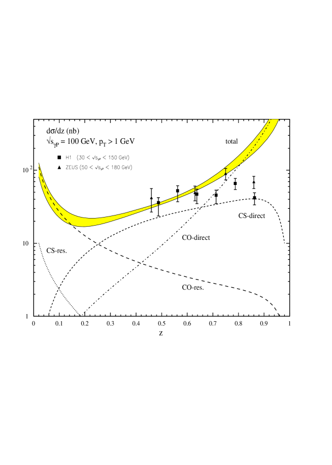
Figure 1: Colour-singlet (CS) and colour-octet (CO) contributions due to direct and resolved photons to the $J/\psi$ energy distribution $d\sigma/dz$ at the photon–proton centre-of-mass energy $\sqrt{s_{\gamma p}}=100\,$GeV in comparison with HERA data [18, 38] averaged over the specified range of $\sqrt{s_{\gamma p}}$. The shaded area bounded by the solid lines represents the sum of all contributions according to scenarios I and II for the colour-octet matrix elements. The lines corresponding to separate colour-octet contributions are plotted for $\langle{\cal O}_{8}^{J/\psi}(^{1}\!S_{0})\rangle=\langle{\cal O}_{8}^{J/\psi}(^{3}\!P_{0})\rangle/m_{c}^{2}=0.008\,\mbox{GeV}^{3}$. The colour-singlet cross section is evaluated in leading order in $\alpha_{s}$. Other parameters: $m_{c}=1.5\,$GeV, renormalisation/factorisation scale $\mu=2m_{c}$, GRV LO proton and photon parton distributions [41], $\Lambda^{(4)}_{LO}=200\,$MeV.

The normalisation of the short-distance cross sections is strongly affected by the choice of the charm quark mass, the QCD coupling, the renormalisation/factorisation scale $\mu$, and the parton distribution functions. Varying the parameters in the range $1.35\,\mbox{GeV}\!<\!m_{c}\!<\!1.65\,\mbox{GeV}$, $m_{c}\!<\!\mu\!<\!4m_{c}$, and $150\,\mbox{MeV}\!<\!\Lambda^{(4)}\!<\!250\,\mbox{MeV}$, the normalisation of $d\hat{\sigma}(ij\to c\bar{c}[n])$ is altered by $\sim\pm 50\%$ around the central value at $m_{c}=1.5$ GeV, $\mu=2m_{c}$, and $\Lambda^{(4)}=200$ MeV. Adopting e.g. the MRS(R2) set of parton distributions [43] and the corresponding value of $\alpha_{s}$ decreases the short-distance cross sections by about a factor of 2 as compared to the leading-order GRV parametrisation. However, the values of the non-perturbative colour-octet matrix elements as extracted from fits to the Tevatron data [26] depend on the choice of $m_{c}$, $\alpha_{s}$, $\mu$ and the parton distribution in approximately the opposite way such as to compensate the change in the short-distance cross section. At leading-twist and leading order in $\alpha_{s}$, the overall normalisation uncertainty of the colour-octet contributions to $J/\psi$ photoproduction is thus in the range of only about $\pm 10\%$, if the short-distance cross sections are multiplied with non-perturbative matrix elements that have been extracted from hadroproduction data using the same set of input parameters. The long-distance factor of the colour-singlet cross section $\langle{\cal O}_{1}^{J/\psi}(^{3}\!S_{1})\rangle$ on the other hand can be determined from the leptonic decay width and is not very sensitive to the choice of parameters, up to unknown contributions from next-to-next-to-leading-order QCD corrections. Consequently, the normalisation uncertainty of the short-distance cross section $d\hat{\sigma}(ij\to c\bar{c}[^{3}\!S_{1}^{(1)}])$ is not compensated by a change in the long-distance factor and the colour-singlet contribution should be considered uncertain within a factor of two. Next-to-leading order QCD corrections [9] increase the colour-singlet cross section by $\sim 20\%\!-\!40\%$, depending in detail on the choice of parameters, but do not affect the shape of the $J/\psi$ energy distribution.

Given the large normalisation uncertainties in particular of the colour-singlet contribution, no conclusive statement about the size of the colour-octet matrix elements can be derived from the $J/\psi$ energy distribution in the region $z\;\hbox to0.0pt{\lower 3.5pt\hbox{$\mathchar 0\relax\sim$}\hss}\raise 1.0pt\hbox{$<$}\;0.8$. On the other hand, the dramatic increase of the colour-octet cross section at larger $z$ is not supported by the data. One should not interpret this discrepancy as a failure of the NRQCD theory itself, but rather as an artefact of our leading-order approximation in $\alpha_{s}$ and $v^{2}$ for the colour-octet contributions. Close to the boundary of phase space, for $z\;\hbox to0.0pt{\lower 3.5pt\hbox{$\mathchar 0\relax\sim$}\hss}\raise 1.0pt\hbox{$>$}\;0.75$, the shape of the $z$-distribution cannot be predicted without resumming singular higher-order terms in the velocity expansion [15]. This difficulty is exactly analogous to the well-known problem of extracting the CKM matrix element $|V_{ub}|$ from the endpoint region of the lepton energy distribution in semileptonic $B$ decay. To constrain the colour-octet contributions from the $J/\psi$ $z$-distribution, the distribution would have to be averaged close to the endpoint over a region much larger than $v^{2}\sim 0.25$.

The low-$z$ region is not expected to be sensitive to higher-order terms in the velocity expansion. Therefore, if the data could be extended to the low-$z$ region, an important resolved photon contribution should be visible, if the colour-octet matrix elements are not significantly smaller than assumed in Table 1.

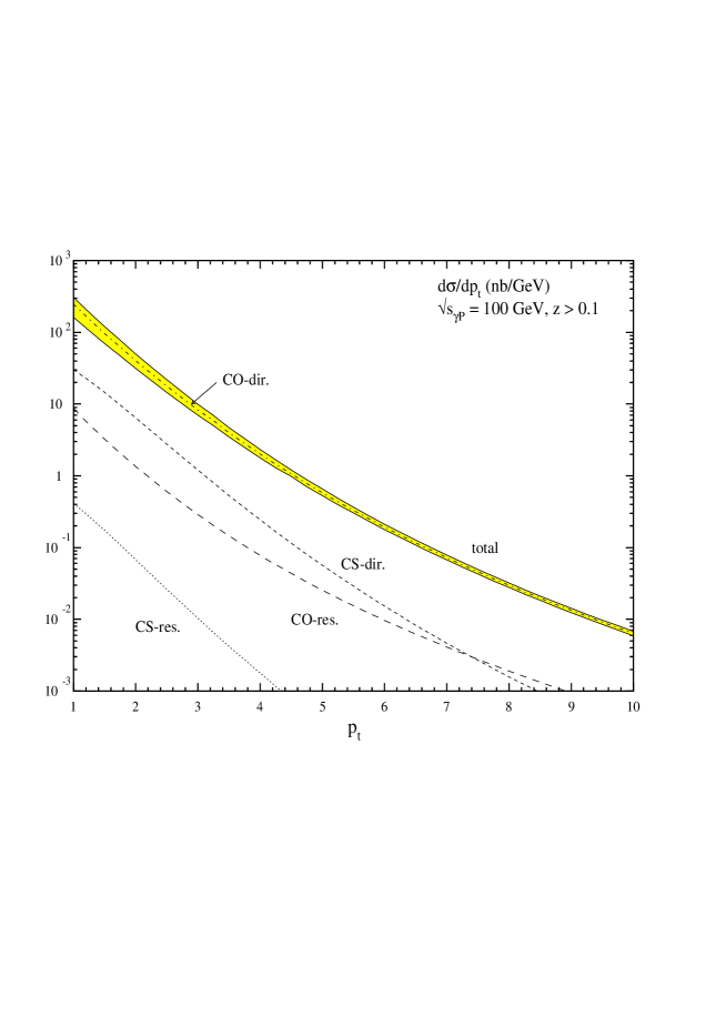
Figure 2: Colour-singlet (CS) and colour-octet (CO) contributions due to direct and resolved photons to the $J/\psi$ transverse momentum distribution $d\sigma/dp_{t}$ at the photon–proton centre-of-mass energy $\sqrt{s_{\gamma p}}=100\,$GeV; $z$ is integrated to its upper kinematic limit. Other specifications are as in Figure 1.

The $p_{t}$-distribution for inelastically produced $J/\psi$ is shown in Figure 2 with a lower $z$-cut: $z>0.1$. As discussed in Section 3 no upper cut in $z$ is necessary or advisable to suppress the diffractive contribution, if the transverse momentum is above about $1\,$GeV. With this definition the differential cross section is dominated by colour-octet contributions, which exceed the colour-singlet contribution by almost an order of magnitude, similar to their significance in hadron–hadron collisions at fixed-target energies [23]. Experimental data from HERA exist only for $p_{t}<3\,$ GeV [18, 38]. The data are presented with a cut at $z<0.9$, in which case the differential cross section at $p_{t}=1\,$GeV ($3\,$GeV) is found to be about a factor of 10 (2) smaller than in Figure 2. The transverse momentum distribution at $z<0.9$ is adequately accounted for by the colour-singlet channel, including next-to-leading-order corrections in $\alpha_{s}$ [9]. Diagrams with $t$-channel gluon exchange lead to large $K$-factors that increase with increasing transverse momentum and harden the $p_{t}$-spectrum of the colour-singlet channel at NLO considerably. We do not expect a similar strong impact of next-to-leading order QCD corrections on the transverse momentum distribution of the colour-octet cross sections. It would be interesting to learn whether including all $z$ can lead to stringent constraints on the size of the colour-octet matrix elements. However, in order to obtain an accurate theoretical prediction in the lower-$p_{t}$ region, $p_{t}\;\hbox to0.0pt{\lower 3.5pt\hbox{$\mathchar 0\relax\sim$}\hss}\raise 1.0pt\hbox{$<$}\;2$–$3\,$GeV, perturbative soft-gluon resummation would have to be taken into account. We expect that soft-gluon resummation will be more important for the colour-octet processes, because there is no Sudakov form factor for radiation off the $c\bar{c}$ pair in the colour-singlet ${}^{3}\!S_{1}$ channel, for which there exists a colour dipole moment only.

4.2 Decay angular distributions

We now turn to the decay angular distributions, which constitute the main result of this work. Below we present the $z$- and $p_{t}$-dependence of the polar and azimuthal decay angular distribution parameters $\lambda,\mu,\nu$ defined in (16), at a typical HERA centre-of-mass energy of $\sqrt{s}=100$ GeV. The quasi-real photons at HERA are actually not mono-energetic, but have a distribution in energy given approximately by the Weizsäcker–Williams approximation. However, in general we have found little energy dependence in the energy range relevant to HERA (the only exception being the predictions in the recoil frame at $z\;\hbox to0.0pt{\lower 3.5pt\hbox{$\mathchar 0\relax\sim$}\hss}\raise 1.0pt\hbox{$<$}\;0.3$) and thus considered a single energy.

Since the decay angular distribution parameters are normalised, the dependence on parameters that affect the absolute normalisation of cross sections, such as the charm quark mass, strong coupling, the renormalisation/factorisation scale and parton distribution, cancels to a large extent and does not constitute a significant uncertainty.

The parameters $\lambda,\mu,\nu$ as function of $z$ are shown in Figures 3-5, which include direct and resolved photon contributions. We computed the decay angular distribution parameters in four commonly used frames (recoil or $s$-channel helicity frame, Gottfried–Jackson frame, target frame and Collins–Soper frame) defined in Appendix A. Each plot exhibits the result from the colour-singlet channel alone (dashed line) and the result after including the colour-octet contributions. The two solid lines correspond to the two scenarios for the colour-octet matrix elements discussed in Section 3. Recall that the $J/\psi$ is unpolarised, if it originates from a $c\bar{c}$ pair in a ${}^{1}\!S_{0}$ state. Thus, in scenario I the angular parameters $\lambda,\mu,\nu$ tend to zero in regions where the colour-octet processes dominate.

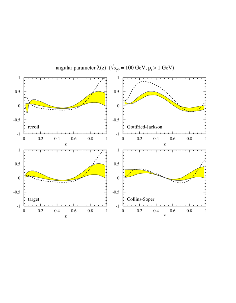
Figure 3: Angular parameter $\lambda$ of the decay angular distribution as a function of $z$. Direct and resolved photons are included. The dashed line is the colour-singlet model prediction. The shaded area shows the NRQCD prediction bounded by the choice of parameters according to scenarios I and II. Other parameters are as in Figure 1.

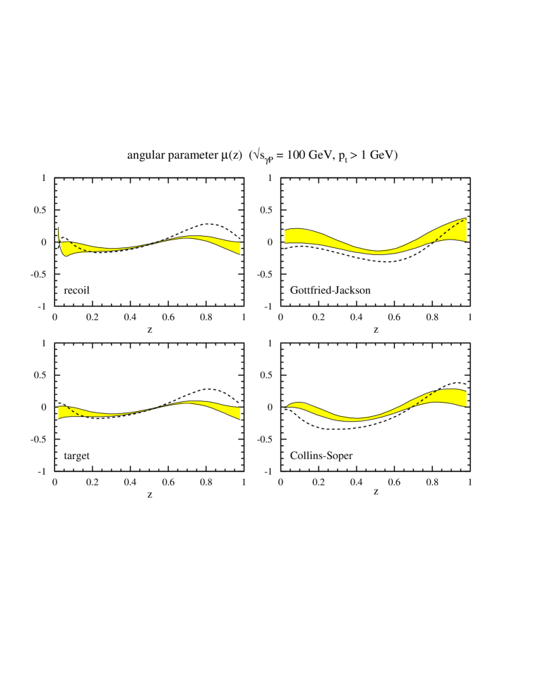
Figure 4: Angular parameter $\mu$ of the decay angular distribution as a function of $z$. Direct and resolved photons are included. The dashed line is the colour-singlet model prediction. The shaded area shows the NRQCD prediction bounded by the choice of parameters according to scenarios I and II. Other parameters are as in Figure 1.

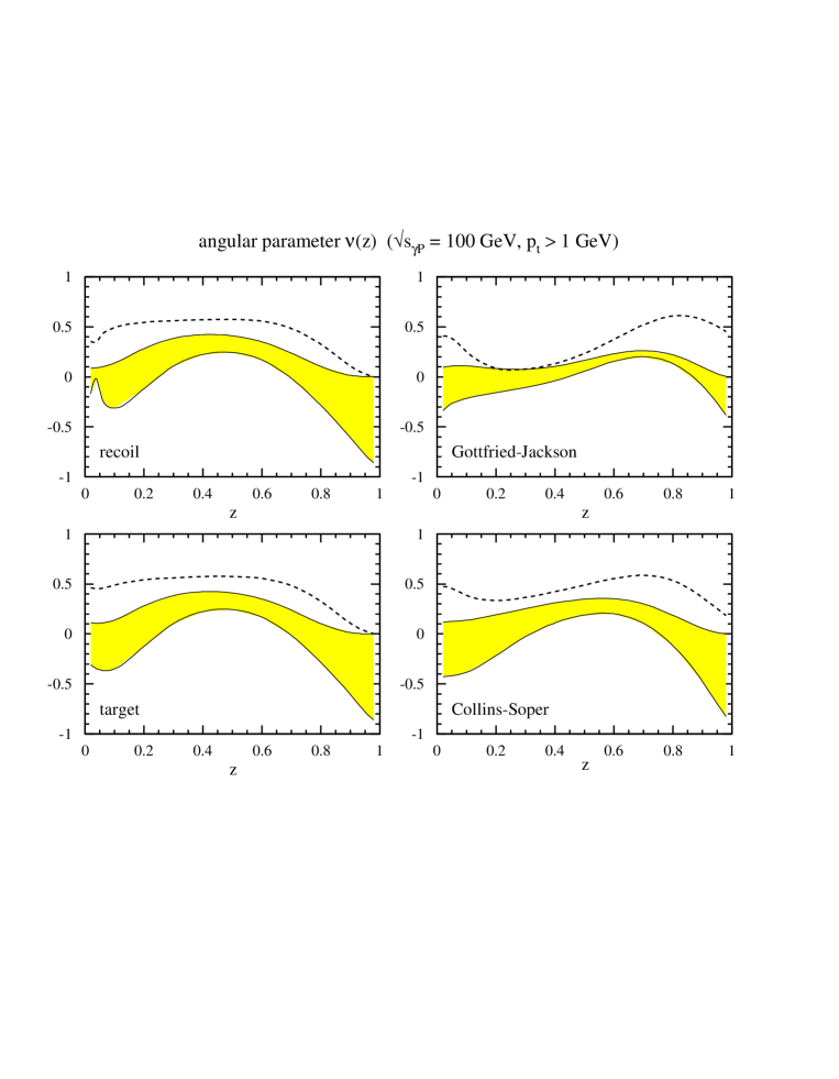
Figure 5: Angular parameter $\nu$ of the decay angular distribution as a function of $z$. Direct and resolved photons are included. The dashed line is the colour-singlet model prediction. The shaded area shows the NRQCD prediction bounded by the choice of parameters according to scenarios I and II. Other parameters are as in Figure 1.

Inspecting Figure 3, we note that in the recoil, target and Collins–Soper frames $\lambda$ differs from the colour-singlet prediction only in the endpoint region. The comparison looks different in the Gottfried–Jackson frame: for $z\;\hbox to0.0pt{\lower 3.5pt\hbox{$\mathchar 0\relax\sim$}\hss}\raise 1.0pt\hbox{$<$}\;0.5$ the colour-singlet channel yields large and positive values of $\lambda$, while the colour-octet contributions yield almost unpolarised $J/\psi$. The azimuthal parameter $\mu$ (Figure 4) turns out to be least interesting. We find that in all frames $\mu$ is relatively flat and close to zero, for both the colour-singlet and colour-octet contributions. The parameter $\nu$, on the other hand, is very different in the colour-singlet channel and after inclusion of colour-octet contributions, even in the intermediate region of $z$, where the colour-singlet channel dominates. As can be seen from Figure 5, this difference is present in all frames and seems to make $\nu$ the most useful parameter to find out about the relative magnitude of colour-singlet and colour-octet contributions experimentally. To determine $\nu$ one could measure the decay angular distribution integrated over the polar angle (cf. (16)),

$$\frac{d\sigma}{d\phi dy}\propto 1+\frac{\lambda(y)}{3}+\frac{\nu(y)}{3}\cos 2\phi,$$ (18)

or project on $\nu$ as follows:

$$\nu(y)=\frac{8}{3}\cdot\frac{\int d\Omega\cos(2\phi)\frac{d\sigma}{d\Omega dy}}{\int d\Omega\left(1-\frac{5}{3}\cos^{2}\theta\right)\frac{d\sigma}{d\Omega dy}}.$$ (19)

A distinctive signature of colour-octet contributions in the large-$z$ region could be of interest in connection with the difficulties in predicting the total cross section in the endpoint region. However, the endpoint region in Figures 3-5 is not without problems either. The higher-order terms in the velocity expansion that need to be resummed close to the endpoint lead to a convolution of the $z$-distribution with certain non-perturbative shape functions. These shape functions depend on the production channel (${}^{3}\!S_{1}^{(1)}$, ${}^{1}\!S_{0}^{(8)}$ and ${}^{3}\!P_{J}^{(8)}$) but they are the same for all density matrix elements in every given production channel.

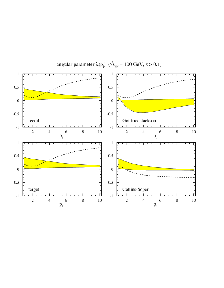
Figure 6: Angular parameter $\lambda$ of the decay angular distribution as a function of $p_{t}$. Direct and resolved photons are included. The dashed line is the colour-singlet model prediction. The shaded area shows the NRQCD prediction bounded by the choice of parameters according to scenarios I and II. Other parameters are as in Figure 1.

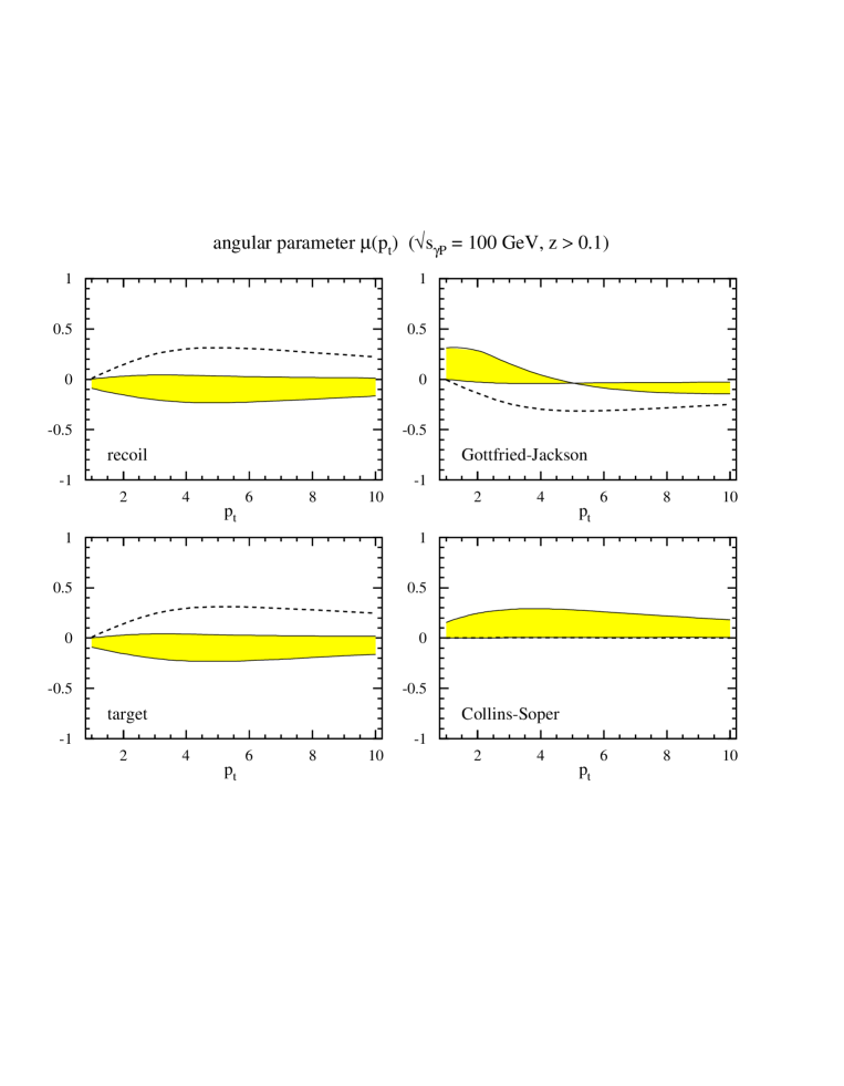
Figure 7: Angular parameter $\mu$ of the decay angular distribution as a function of $p_{t}$. Direct and resolved photons are included. The dashed line is the colour-singlet model prediction. The shaded area shows the NRQCD prediction bounded by the choice of parameters according to scenarios I and II. Other parameters are as in Figure 1.

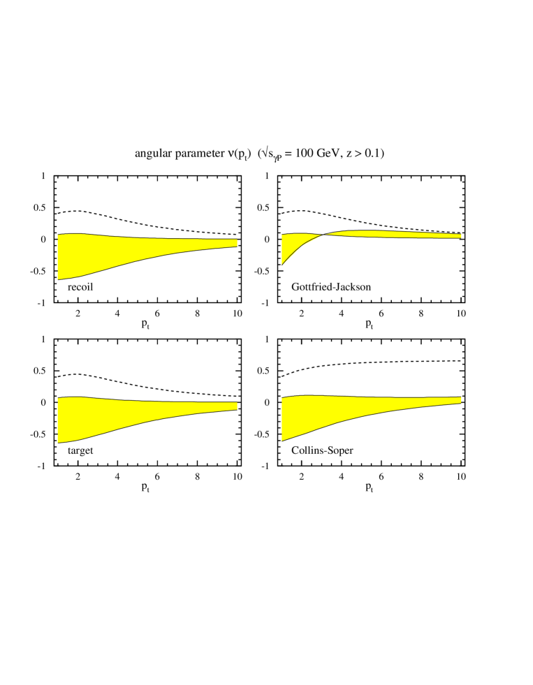
Figure 8: Angular parameter $\nu$ of the decay angular distribution as a function of $p_{t}$. Direct and resolved photons are included. The dashed line is the colour-singlet model prediction. The shaded area shows the NRQCD prediction bounded by the choice of parameters according to scenarios I and II. Other parameters are as in Figure 1.

As a consequence, while the energy distribution itself depends on these shape functions, the moments in $z$ of the normalised angular parameters depend only on the difference of the shape functions in the various production channels. Since we do expect such differences, especially between the colour-singlet and the colour-octet channels (due to the different properties with respect to soft gluon radiation), and since we are interested in the $z$-distribution rather than its moments, the predictions for the angular parameters in the endpoint region still depend on these shape functions. However, this dependence is strong only if the angular parameter varies strongly in the endpoint region and disappears entirely if its distribution is flat.

In Figures 6-8 we present the same analysis for the $p_{t}$-distribution. We note that $z$ is integrated up to its kinematic maximum. As a consequence the cross section is colour-octet dominated and the colour-singlet contribution plays no role for the solid curves. Since the colour-octet cross section is dominated by the large-$z$ region, the solid curves are entirely determined by the polarisation yield of octet mechanisms at large $z$. Contrary to the situation of hadroproduction at the Tevatron, where one expects large transverse polarisation due to gluon fragmentation into colour-octet $c\bar{c}$ pairs [24], the photoproduction cross section tends to be unpolarised in the $p_{t}$ region considered here. Therefore, the $p_{t}$-distributions do not discriminate between the theoretical prediction based on NRQCD and that of the colour evaporation model, which always predicts unpolarised $J/\psi$.

On the other hand, the transverse momentum distribution seems to prove very useful to determine the relative magnitude of colour-singlet and colour-octet contributions: If the cross section is dominated by the colour-singlet channel, large and positive values of the polar angular parameter $\lambda$ (Figure 6) are expected for $p_{t}\;\hbox to0.0pt{\lower 3.5pt\hbox{$\mathchar 0\relax\sim$}\hss}\raise 1.0pt\hbox{$>$}\;5$ GeV in the recoil, Gottfried–Jackson and target frames. A similar distinctive difference between colour-singlet and colour-octet channels is visible in the azimuthal parameter $\nu$ as defined in the Collins–Soper frame, see Figure 8.

The unique transverse polarisation signature of gluon fragmentation could possibly be made visible in the resolved photon contribution. If the direct photon contribution is reduced by a cut on the high-$z$ region, the resolved cross section is dominated by $g\to c\bar{c}[^{3}\!S_{1}^{(8)}]$ at large transverse momentum [16]. As for hadroproduction [29, 26], we expect that $p_{t}\;\hbox to0.0pt{\lower 3.5pt\hbox{$\mathchar 0\relax\sim$}\hss}\raise 1.0pt\hbox{$>$}\;(5$–$10)\,$GeV is necessary to suppress sufficiently the other colour-octet channels.

5 Conclusion

We presented an analysis of the full polar and azimuthal decay angular distributions of inelastically photo-produced $J/\psi$ based on the NRQCD factorisation approach to quarkonium production. The primary motivation of this study is to find observables in addition to angular-integrated differential cross sections, which are sensitive to different theories and models of quarkonium production. A particular emphasis is on clarifying the role of colour-octet contributions suggested by NRQCD and other quarkonium production processes in comparison with the colour-singlet model, which can be considered as a successful description of photoproduction as far as present, limited, data on energy and transverse momentum distributions is concerned.

Assuming NRQCD long-distance parameters as constrained by other $J/\psi$ production processes such as in hadroproduction and $B$ decay, we have found that the azimuthal decay angle distribution as a function of $z$ or $p_{t}$ would be extremely useful for discriminating between the colour-singlet model and NRQCD and, to a lesser extent, the colour evaporation model. We also noted that transverse-momentum distributions integrated over all energy fraction $z$ are colour-octet dominated and could give meaningful constraints on colour-octet matrix elements from the angular integrated rate as well as the decay angle dependence.

While this paper was being written, Fleming and Mehen [44] presented a study of leptoproduction of $J/\psi$ in NRQCD, which is complementary to our photoproduction analysis. Contrary to photoproduction, the leading-twist partonic diagrams at $O(\alpha\alpha_{s})$ can be sensibly compared with a total leptoproduction cross section for large enough photon virtuality $Q^{2}$. Fleming and Mehen computed the polar angle distribution due to these leading-order mechanisms and also find interesting tests of NRQCD.

Acknowledgements. We would like to thank J.G. Körner for useful discussions. M.B. wishes to thank John Collins for supplying a FORTRAN integration routine.

Appendix A Polarisation frames

We collect here the covariant expressions for polarisation vectors in the four commonly used frames, following [45]. (Note that the metric $g_{\mu\nu}=\mbox{diag}(-1,1,1,1)$ is used there.)

Let $p_{\gamma}$ be the photon momentum, $p_{p}$ the proton momentum, $P$ the momentum of quarkonium $\psi$ and $s=(p_{\gamma}+p_{p})^{2}$. We define the auxiliary vectors

$$A=p_{\gamma}+p_{p}\qquad\tilde{A}^{\mu}=A^{\mu}-\frac{A\cdot PP^{\mu}}{M^{2}},$$ (20)

$$B=p_{\gamma}-p_{p}\qquad\tilde{B}^{\mu}=B^{\mu}-\frac{B\cdot PP^{\mu}}{M^{2}},$$ (21)

where $M$ is the $\psi$ mass. (We take $M=2m_{c}$ in the analysis. The proton mass will be neglected in the following.) Note that $\tilde{A}$, $\tilde{B}$ are three-vectors in the $\psi$-rest frame. We then define a coordinate system as follows:

1. Choose $Z^{\mu}=\alpha_{z}\tilde{A}^{\mu}+\beta_{z}\tilde{B}^{\mu}$, with $Z^{2}=-1$.

2. Define $X^{\mu}=\alpha_{x}\tilde{A}^{\mu}+\beta_{x}\tilde{B}^{\mu}$ in the plane spanned by $\tilde{A}$, $\tilde{B}$, orthogonal to $Z$ and normalised: $X\cdot Z=0$, $X^{2}=-1$.

3. Take $Y$ to complete a right-handed coordinate system in the $\psi$-rest frame,

   $$Y^{\mu}=\frac{1}{M}\epsilon^{\mu\alpha\beta\gamma}P_{\alpha}X_{\beta}Z_{\gamma}$$ (22)

   ($\epsilon^{0123}=1$). The sign ambiguity in $\alpha_{x}$, $\beta_{x}$ left in the second step is fixed by requiring $\vec{Y}$ to point in the direction of $\vec{p_{\gamma}}\times(-\vec{p}_{p})$ in the $\psi$-rest frame, which requires $\alpha_{z}\beta_{x}-\alpha_{x}\beta_{z}>0$.

The four commonly used polarisation frames are then specified by the choice of $Z$. In the recoil (or $s$-channel helicity) frame, the $Z$-axis is defined as the direction of the $\psi$ three-momentum in the hadronic centre-of-mass frame, that is $\vec{Z}=-\vec{A}/|\vec{A}|$ in the $\psi$-rest frame. In the Gottfried–Jackson frame $\vec{Z}=\vec{p}_{\gamma}/|\vec{p}_{\gamma}|$ and in the target frame $\vec{Z}=-\vec{p}_{p}/|\vec{p}_{p}|$. In the Collins–Soper frame the $Z$-axis bisects the angle between $\vec{p}_{\gamma}$ and $(-\vec{p}_{p})$, i.e. $\vec{Z}\propto\vec{p}_{\gamma}/|\vec{p}_{\gamma}|+(-\vec{p}_{p})/|\vec{p}_{p}|$. (All three-vectors refer to the $\psi$-rest frame.) We then find the covariant expressions for the coordinate axes from the following expressions for $\alpha_{z,x}$, $\beta_{z,x}$:

Recoil frame:

$$\alpha_{z}=-\frac{M}{\sqrt{(A\cdot P)^{2}-M^{2}s}}\qquad\beta_{z}=0$$ (23)

$$\alpha_{x} = \frac{A\cdot PB\cdot P}{\sqrt{s\,((A\cdot P)^{2}-M^{2}s)((A\cdot P)^{2}-(B\cdot P)^{2}-M^{2}s)}}$$ (24)

$$\beta_{x} = -\frac{\sqrt{(A\cdot P)^{2}-M^{2}s}}{\sqrt{s\,((A\cdot P)^{2}-(B\cdot P)^{2}-M^{2}s)}}$$ (25)

Gottfried–Jackson frame:

$$\alpha_{z}=\beta_{z}=\frac{M}{A\cdot P+B\cdot P}$$ (26)

$$\alpha_{x} = -\frac{(B\cdot P)^{2}+A\cdot PB\cdot P+M^{2}s}{(A\cdot P+B\cdot P)\sqrt{s\,((A\cdot P)^{2}-(B\cdot P)^{2}-M^{2}s)}}$$ (27)

$$\beta_{x} = \frac{(A\cdot P)^{2}+A\cdot PB\cdot P-M^{2}s}{(A\cdot P+B\cdot P)\sqrt{s\,((A\cdot P)^{2}-(B\cdot P)^{2}-M^{2}s)}}$$ (28)

Target frame:

$$\alpha_{z}=-\beta_{z}=-\frac{M}{A\cdot P-B\cdot P}$$ (29)

$$\alpha_{x} = -\frac{(B\cdot P)^{2}-A\cdot PB\cdot P+M^{2}s}{(A\cdot P-B\cdot P)\sqrt{s\,((A\cdot P)^{2}-(B\cdot P)^{2}-M^{2}s)}}$$ (30)

$$\beta_{x} = -\frac{(A\cdot P)^{2}-A\cdot PB\cdot P-M^{2}s}{(A\cdot P-B\cdot P)\sqrt{s\,((A\cdot P)^{2}-(B\cdot P)^{2}-M^{2}s)}}$$ (31)

Collins–Soper frame:

$$\alpha_{z}=-\frac{B\cdot P}{\sqrt{s\,((A\cdot P)^{2}-(B\cdot P)^{2})}}\qquad\beta_{z}=\frac{A\cdot P}{\sqrt{s\,((A\cdot P)^{2}-(B\cdot P)^{2})}}$$ (32)

$$\alpha_{x} = -\frac{M\,A\cdot P}{\sqrt{((A\cdot P)^{2}-(B\cdot P)^{2})\,((A\cdot P)^{2}-(B\cdot P)^{2}-M^{2}s)}}$$ (33)

$$\beta_{x} = \frac{M\,B\cdot P}{\sqrt{((A\cdot P)^{2}-(B\cdot P)^{2})\,((A\cdot P)^{2}-(B\cdot P)^{2}-M^{2}s)}}$$ (34)

We note that $A\cdot P+B\cdot P=(P_{t}^{2}+M^{2})/z$ and $A\cdot P-B\cdot P=sz$. Finally, the polarisation vectors are given by

$$\epsilon^{\mu}(\lambda=0)=Z^{\mu}\qquad\epsilon^{\mu}(\lambda=\pm 1)=\frac{1}{\sqrt{2}}(\mp X^{\mu}-iY^{\mu}).$$ (35)

Appendix B Density matrices

The density matrices for all processes considered in the paper are given in this Appendix. The results given for the resolved photon process apply equally to $J/\psi$ production in hadron-hadron collisions and have been used in [26]. The functions $F,a,b,c,d$ below are related to $A,B,C,D$ of (15) as $A=Fa$ etc., and we suppressed all sub- and superscripts. For the partonic process $1+2\to 3+4$, the Mandelstam invariants are $\hat{s}=(p_{1}+p_{2})^{2}$, $\hat{t}=(p_{3}-p_{1})^{2}$, $\hat{u}=(p_{3}-p_{2})^{2}$.

B.1 Direct-photon processes

$\gamma+g\rightarrow c\bar{c}\left[{}^{3}\!S_{1}^{(1)}\right]+g$:

$$F = \frac{16M(4\pi)^{3}\alpha\alpha_{s}^{2}e_{c}^{2}\langle{\cal O}_{1}^{J/\psi}(^{3}\!S_{1})\rangle}{27[(\hat{s}-M^{2})(\hat{t}-M^{2})(\hat{u}-M^{2})]^{2}}$$ (36)

$$a = -(\hat{s}^{2}+\hat{s}\hat{t}+\hat{t}^{2})^{2}+M^{2}(2\hat{s}^{2}+\hat{s}\hat{t}+2\hat{t}^{2})(\hat{s}+\hat{t})-M^{4}(\hat{s}^{2}+\hat{s}\hat{t}+\hat{t}^{2})$$ (37)

$$b = -2(\hat{s}^{2}+\hat{t}^{2})$$ (38)

$$c = -2(\hat{s}^{2}+\hat{u}^{2})$$ (39)

$$d = -2\hat{s}^{2}$$ (40)

$\gamma+g\rightarrow c\bar{c}\left[{}^{3}\!S_{1}^{(8)}\right]+g$: $a,b,c,d$ are the same as (37)–(40), $F$ is multiplied by

$$\frac{15}{8}\cdot\frac{\langle{\cal O}_{8}^{J/\psi}(^{3}\!S_{1})\rangle}{\langle{\cal O}_{1}^{J/\psi}(^{3}\!S_{1})\rangle}$$ (41)

$\gamma+g\rightarrow c\bar{c}\left[{}^{1}\!S_{0}^{(8)}\right]+g$:

$$Fa = -\frac{2(4\pi)^{3}\alpha\alpha_{s}^{2}e_{c}^{2}\langle{\cal O}_{8}^{J/\psi}(^{1}\!S_{0})\rangle}{M\hat{t}[(\hat{s}-M^{2})(\hat{t}-M^{2})(\hat{u}-M^{2})]^{2}}$$ (42)

$$\times\hat{s}\hat{u}\left\{[\hat{u}^{2}-M^{2}(\hat{u}-M^{2})]^{2}-2\hat{s}\hat{t}(\hat{u}-M^{2})^{2}+\hat{s}^{2}\hat{t}^{2}\right\}$$

$$b = c=d=0$$ (43)

$\gamma+g\rightarrow c\bar{c}\left[{}^{3}\!P_{J}^{(8)}\right]+g$:

$$F = -\frac{24(4\pi)^{3}\alpha\alpha_{s}^{2}e_{c}^{2}\langle{\cal O}_{8}^{J/\psi}(^{3}\!P_{0})\rangle}{\hat{t}^{2}[M(\hat{s}-M^{2})(\hat{t}-M^{2})(\hat{u}-M^{2})]^{3}}$$ (44)

$$a = \hat{s}^{2}\hat{t}^{2}(\hat{s}+\hat{t})^{2}(\hat{s}^{2}+\hat{s}\hat{t}+\hat{t}^{2})^{2}$$ (45)

$$\mbox{}-M^{2}\hat{s}\hat{t}(\hat{s}^{7}+8\hat{s}^{6}\hat{t}+16\hat{s}^{5}\hat{t}^{2}+16\hat{s}^{4}\hat{t}^{3}+8\hat{s}^{3}\hat{t}^{4}-3\hat{s}\hat{t}^{6}-2\hat{t}^{7})$$

$$\mbox{}+M^{4}\hat{t}(4\hat{s}^{7}+28\hat{s}^{6}\hat{t}+48\hat{s}^{5}\hat{t}^{2}+41\hat{s}^{4}\hat{t}^{3}+18\hat{s}^{3}\hat{t}^{4}-4\hat{s}\hat{t}^{6}+\hat{t}^{7})$$

$$\mbox{}-M^{6}\hat{t}(12\hat{s}^{6}+64\hat{s}^{5}\hat{t}+99\hat{s}^{4}\hat{t}^{2}+80\hat{s}^{3}\hat{t}^{3}+33\hat{s}^{2}\hat{t}^{4}+3\hat{s}\hat{t}^{5}+3\hat{t}^{6})$$

$$\mbox{}+M^{8}\hat{t}(22\hat{s}^{5}+88\hat{s}^{4}\hat{t}+114\hat{s}^{3}\hat{t}^{2}+67\hat{s}^{2}\hat{t}^{3}+14\hat{s}\hat{t}^{4}+3\hat{t}^{5})$$

$$\mbox{}-M^{10}\hat{t}(22\hat{s}^{4}+68\hat{s}^{3}\hat{t}+61\hat{s}^{2}\hat{t}^{2}+16\hat{s}\hat{t}^{3}+\hat{t}^{4})$$

$$\mbox{}+2M^{12}\hat{s}\hat{t}(6\hat{s}^{2}+13\hat{s}\hat{t}+5\hat{t}^{2})-3M^{14}\hat{s}\hat{t}(\hat{s}+\hat{t})$$

$$b = -2(\hat{s}+\hat{t})^{4}(2\hat{s}^{4}+\hat{s}^{2}\hat{t}^{2}+2\hat{t}^{4})$$ (46)

$$\mbox{}+2M^{2}(6\hat{s}^{7}+19\hat{s}^{6}\hat{t}+21\hat{s}^{5}\hat{t}^{2}+17\hat{s}^{4}\hat{t}^{3}+21\hat{s}^{3}\hat{t}^{4}+28\hat{s}^{2}\hat{t}^{5}+22\hat{s}\hat{t}^{6}+6\hat{t}^{7})$$

$$\mbox{}-2M^{4}(6\hat{s}^{6}+9\hat{s}^{5}\hat{t}-15\hat{s}^{4}\hat{t}^{2}-24\hat{s}^{3}\hat{t}^{3}-4\hat{s}^{2}\hat{t}^{4}+15\hat{s}\hat{t}^{5}+5\hat{t}^{6})$$

$$\mbox{}+2M^{6}(2\hat{s}^{5}-10\hat{s}^{4}\hat{t}-45\hat{s}^{3}\hat{t}^{2}-37\hat{s}^{2}\hat{t}^{3}-3\hat{s}\hat{t}^{4}+\hat{t}^{5})$$

$$\mbox{}+8M^{8}\hat{s}\hat{t}(3\hat{s}^{2}+7\hat{s}\hat{t}+2\hat{t}^{2})-8M^{10}\hat{s}\hat{t}(\hat{s}+\hat{t})$$

$$c = 2\hat{t}^{2}(2\hat{s}^{6}+6\hat{s}^{5}\hat{t}+5\hat{s}^{4}\hat{t}^{2}-7\hat{s}^{2}\hat{t}^{4}-6\hat{s}\hat{t}^{5}-2\hat{t}^{6})$$ (47)

$$\mbox{}+2M^{2}\hat{t}^{2}(-6\hat{s}^{5}-9\hat{s}^{4}\hat{t}+2\hat{s}^{3}\hat{t}^{2}+21\hat{s}^{2}\hat{t}^{3}+22\hat{s}\hat{t}^{4}+8\hat{t}^{5})$$

$$\mbox{}-2M^{4}(2\hat{s}^{6}+6\hat{s}^{5}\hat{t}-11\hat{s}^{4}\hat{t}^{2}-20\hat{s}^{3}\hat{t}^{3}+7\hat{s}^{2}\hat{t}^{4}+27\hat{s}\hat{t}^{5}+11\hat{t}^{6})$$

$$\mbox{}+2M^{6}(6\hat{s}^{5}+15\hat{s}^{4}\hat{t}-12\hat{s}^{3}\hat{t}^{2}-19\hat{s}^{2}\hat{t}^{3}+8\hat{s}\hat{t}^{4}+4\hat{t}^{5})$$

$$\mbox{}-4M^{8}(3\hat{s}^{4}+6\hat{s}^{3}\hat{t}-4\hat{s}^{2}\hat{t}^{2}-3\hat{s}\hat{t}^{3}-2\hat{t}^{4})$$

$$\mbox{}+4M^{10}(\hat{s}^{3}+2\hat{s}^{2}\hat{t}-\hat{s}\hat{t}^{2}-2\hat{t}^{3})-2M^{12}\hat{t}(\hat{s}-\hat{t})$$

$$d = 2\hat{t}^{2}(\hat{s}^{6}+2\hat{s}^{5}\hat{t}-6\hat{s}^{3}\hat{t}^{3}-10\hat{s}^{2}\hat{t}^{4}-7\hat{s}\hat{t}^{5}-2\hat{t}^{6})$$ (48)

$$\mbox{}-M^{2}(4\hat{s}^{7}+14\hat{s}^{6}\hat{t}+30\hat{s}^{5}\hat{t}^{2}+29\hat{s}^{4}\hat{t}^{3}+4\hat{s}^{3}\hat{t}^{4}-33\hat{s}^{2}\hat{t}^{5}-38\hat{s}\hat{t}^{6}-14\hat{t}^{7})$$

$$\mbox{}+2M^{4}(6\hat{s}^{6}+21\hat{s}^{5}\hat{t}+43\hat{s}^{4}\hat{t}^{2}+43\hat{s}^{3}\hat{t}^{3}+13\hat{s}^{2}\hat{t}^{4}-15\hat{s}\hat{t}^{5}-9\hat{t}^{6})$$

$$\mbox{}-M^{6}(12\hat{s}^{5}+45\hat{s}^{4}\hat{t}+92\hat{s}^{3}\hat{t}^{2}+78\hat{s}^{2}\hat{t}^{3}+6\hat{s}\hat{t}^{4}-9\hat{t}^{5})$$

$$\mbox{}+2M^{8}\hat{s}(2\hat{s}^{3}+11\hat{s}^{2}\hat{t}+22\hat{s}\hat{t}^{2}+9\hat{t}^{3})-M^{10}\hat{t}(5\hat{s}^{2}+6\hat{s}\hat{t}+\hat{t}^{2})$$

$\gamma+q\rightarrow c\bar{c}\left[{}^{3}\!S_{1}^{(8)}\right]+q$:

$$F = \frac{(4\pi)^{3}\alpha\alpha_{s}^{2}e_{q}^{2}\langle{\cal O}_{8}^{J/\psi}(^{3}\!S_{1})\rangle}{9M^{3}\hat{s}\hat{u}}$$ (49)

$$a = \hat{s}^{2}+\hat{u}^{2}+2M^{2}\hat{t}$$ (50)

$$b = 4$$ (51)

$$c = 8$$ (52)

$$d = 4,$$ (53)

where $e_{q}$ is the electric charge of the light quark $q$.

$\gamma+q\rightarrow c\bar{c}\left[{}^{1}\!S_{0}^{(8)}\right]+q$:

$$Fa = \frac{4(4\pi)^{3}\alpha\alpha_{s}^{2}e_{c}^{2}\langle{\cal O}_{8}^{J/\psi}(^{1}\!S_{0})\rangle}{9M\hat{t}(\hat{t}-M^{2})^{2}}\,\left\{\hat{s}^{2}+\hat{u}^{2}\right\}$$ (54)

$$b = c=d=0$$ (55)

$\gamma+q\rightarrow c\bar{c}\left[{}^{3}\!P_{J}^{(8)}\right]+q$:

$$F = \frac{16(4\pi)^{3}\alpha\alpha_{s}^{2}e_{c}^{2}\langle{\cal O}_{8}^{J/\psi}(^{3}\!P_{0})\rangle}{3M^{3}\hat{t}^{2}(\hat{t}-M^{2})^{3}}$$ (56)

$$a = \hat{t}(\hat{t}-M^{2})(\hat{s}^{2}+\hat{u}^{2}+2M^{2}\hat{t}+2M^{4})$$ (57)

$$b = -8(\hat{s}^{2}+\hat{s}\hat{t}+M^{2}\hat{t})$$ (58)

$$c = 8(\hat{t}^{2}-M^{4})$$ (59)

$$d = 4(\hat{t}^{2}-2M^{2}\hat{s}-M^{2}\hat{t})$$ (60)

B.2 Resolved-photon processes

$g+g\rightarrow c\bar{c}\left[{}^{3}S_{1}^{(1)}\right]+g$: $a,b,c,d$ are the same as (37)–(40), $F$ is multiplied by

$$\frac{5}{96}\cdot\frac{\alpha_{s}}{\alpha e_{c}^{2}}$$ (61)

$g+g\rightarrow c\bar{c}\left[{}^{3}S_{1}^{(8)}\right]+g$:

$$F = \frac{(4\pi\alpha_{s})^{3}\langle{\cal O}_{8}^{J/\psi}(^{3}\!S_{1})\rangle}{144M^{3}[(\hat{s}-M^{2})(\hat{t}-M^{2})(\hat{u}-M^{2})]^{2}}\,\left\{27(\hat{s}\hat{t}+\hat{s}\hat{u}+\hat{t}\hat{u})-19M^{4}\right\}$$ (62)

$$a = (\hat{s}^{2}+\hat{s}\hat{t}+\hat{t}^{2})^{2}-M^{2}(2\hat{s}^{2}+\hat{s}\hat{t}+2\hat{t}^{2})(\hat{s}+\hat{t})+M^{4}(\hat{s}^{2}+\hat{s}\hat{t}+\hat{t}^{2})$$ (63)

$$b = 2(\hat{s}^{2}+\hat{t}^{2})$$ (64)

$$c = 2(\hat{s}^{2}+\hat{u}^{2})$$ (65)

$$d = 2\hat{s}^{2}$$ (66)

$g+g\rightarrow c\bar{c}\left[{}^{1}S_{0}^{(8)}\right]+g$:

$$Fa = -\frac{5(4\pi\alpha_{s})^{3}\langle{\cal O}_{8}^{J/\psi}(^{1}S_{0})\rangle}{48M\hat{s}\hat{t}\hat{u}[(\hat{s}-M^{2})(\hat{t}-M^{2})(\hat{u}-M^{2})]^{2}}$$ (67)

$$\times\left\{\hat{s}^{2}(\hat{s}-M^{2})^{2}+\hat{s}\hat{t}\hat{u}(M^{2}-2\hat{s})+\hat{t}^{2}\hat{u}^{2}\right\}$$

$$\times\left\{(\hat{s}^{2}-M^{2}\hat{s}+M^{4})^{2}-\hat{t}\hat{u}(2\hat{t}^{2}+3\hat{t}\hat{u}+2\hat{u}^{2})\right\}$$

$$b = c=d=0$$ (68)

$g+g\rightarrow c\bar{c}\left[{}^{3}P_{J}^{(8)}\right]+g$:

$$F = \frac{5(4\pi\alpha_{s})^{3}\langle{\cal O}_{8}^{J/\psi}(^{3}\!P_{0})\rangle}{4\hat{s}^{2}\hat{t}^{2}\hat{u}^{2}[M(\hat{s}-M^{2})(\hat{t}-M^{2})(\hat{u}-M^{2})]^{3}}$$ (69)

$$a = \hat{s}\hat{t}\hat{u}\,\Big{\{}\hat{s}^{10}\hat{t}+5\hat{s}^{9}\hat{t}^{2}+14\hat{s}^{8}\hat{t}^{3}+26\hat{s}^{7}\hat{t}^{4}+35\hat{s}^{6}\hat{t}^{5}+35\hat{s}^{5}\hat{t}^{6}+26\hat{s}^{4}\hat{t}^{7}+14\hat{s}^{3}\hat{t}^{8}$$ (70)

$$\mbox{}+5\hat{s}^{2}\hat{t}^{9}+\hat{s}\hat{t}^{10}$$

$$\mbox{}-M^{2}(\hat{s}^{10}+10\hat{s}^{9}\hat{t}+26\hat{s}^{8}\hat{t}^{2}+40\hat{s}^{7}\hat{t}^{3}+45\hat{s}^{6}\hat{t}^{4}+44\hat{s}^{5}\hat{t}^{5}+45\hat{s}^{4}\hat{t}^{6}$$

$$\mbox{}+40\hat{s}^{3}\hat{t}^{7}+26\hat{s}^{2}\hat{t}^{8}+10\hat{s}\hat{t}^{9}+\hat{t}^{10})$$

$$\mbox{}+M^{4}(5\hat{s}^{9}+40\hat{s}^{8}\hat{t}+84\hat{s}^{7}\hat{t}^{2}+106\hat{s}^{6}\hat{t}^{3}+103\hat{s}^{5}\hat{t}^{4}+103\hat{s}^{4}\hat{t}^{5}+106\hat{s}^{3}\hat{t}^{6}$$

$$\mbox{}+84\hat{s}^{2}\hat{t}^{7}+40\hat{s}\hat{t}^{8}+5\hat{t}^{9})$$

$$\mbox{}-M^{6}(16\hat{s}^{8}+104\hat{s}^{7}\hat{t}+215\hat{s}^{6}\hat{t}^{2}+291\hat{s}^{5}\hat{t}^{3}+316\hat{s}^{4}\hat{t}^{4}+291\hat{s}^{3}\hat{t}^{5}+215\hat{s}^{2}\hat{t}^{6}$$

$$\mbox{}+104\hat{s}\hat{t}^{7}+16\hat{t}^{8})$$

$$\mbox{}+M^{8}(34\hat{s}^{7}+179\hat{s}^{6}\hat{t}+356\hat{s}^{5}\hat{t}^{2}+473\hat{s}^{4}\hat{t}^{3}+473\hat{s}^{3}\hat{t}^{4}+356\hat{s}^{2}\hat{t}^{5}+179\hat{s}\hat{t}^{6}+34\hat{t}^{7})$$

$$\mbox{}-M^{10}(44\hat{s}^{6}+193\hat{s}^{5}\hat{t}+346\hat{s}^{4}\hat{t}^{2}+410\hat{s}^{3}\hat{t}^{3}+346\hat{s}^{2}\hat{t}^{4}+193\hat{s}\hat{t}^{5}+44\hat{t}^{6})$$

$$\mbox{}+M^{12}(34\hat{s}^{5}+124\hat{s}^{4}\hat{t}+188\hat{s}^{3}\hat{t}^{2}+188\hat{s}^{2}\hat{t}^{3}+124\hat{s}\hat{t}^{4}+34\hat{t}^{5})$$

$$\mbox{}-M^{14}(15\hat{s}^{4}+43\hat{s}^{3}\hat{t}+52\hat{s}^{2}\hat{t}^{2}+43\hat{s}\hat{t}^{3}+15\hat{t}^{4})$$

$$\mbox{}+M^{16}(3\hat{s}^{3}+6\hat{s}^{2}\hat{t}+6\hat{s}\hat{t}^{2}+3\hat{t}^{3})\Big{\}}$$

$$b = 4\hat{s}^{12}+24\hat{s}^{11}\hat{t}+68\hat{s}^{10}\hat{t}^{2}+124\hat{s}^{9}\hat{t}^{3}+164\hat{s}^{8}\hat{t}^{4}+176\hat{s}^{7}\hat{t}^{5}+176\hat{s}^{6}\hat{t}^{6}$$ (71)

$$\mbox{}+176\hat{s}^{5}\hat{t}^{7}+164\hat{s}^{4}\hat{t}^{8}+124\hat{s}^{3}\hat{t}^{9}+68\hat{s}^{2}\hat{t}^{10}+24\hat{s}\hat{t}^{11}+4\hat{t}^{12}$$

$$\mbox{}-M^{2}(20\hat{s}^{11}+104\hat{s}^{10}\hat{t}+250\hat{s}^{9}\hat{t}^{2}+397\hat{s}^{8}\hat{t}^{3}+481\hat{s}^{7}\hat{t}^{4}+500\hat{s}^{6}\hat{t}^{5}$$

$$\mbox{}+500\hat{s}^{5}\hat{t}^{6}+481\hat{s}^{4}\hat{t}^{7}+397\hat{s}^{3}\hat{t}^{8}+250\hat{s}^{2}\hat{t}^{9}+104\hat{s}\hat{t}^{10}+20\hat{t}^{11})$$

$$\mbox{}+M^{4}(40\hat{s}^{10}+166\hat{s}^{9}\hat{t}+278\hat{s}^{8}\hat{t}^{2}+285\hat{s}^{7}\hat{t}^{3}+206\hat{s}^{6}\hat{t}^{4}+146\hat{s}^{5}\hat{t}^{5}+206\hat{s}^{4}\hat{t}^{6}$$

$$\mbox{}+285\hat{s}^{3}\hat{t}^{7}+278\hat{s}^{2}\hat{t}^{8}+166\hat{s}\hat{t}^{9}+40\hat{t}^{10})$$

$$\mbox{}+M^{6}(-40\hat{s}^{9}-97\hat{s}^{8}\hat{t}+53\hat{s}^{7}\hat{t}^{2}+373\hat{s}^{6}\hat{t}^{3}+647\hat{s}^{5}\hat{t}^{4}+647\hat{s}^{4}\hat{t}^{5}+373\hat{s}^{3}\hat{t}^{6}+53\hat{s}^{2}\hat{t}^{7}$$

$$\mbox{}-97\hat{s}\hat{t}^{8}-40\hat{t}^{9})$$

$$\mbox{}+M^{8}(20\hat{s}^{8}-33\hat{s}^{7}\hat{t}-368\hat{s}^{6}\hat{t}^{2}-751\hat{s}^{5}\hat{t}^{3}-920\hat{s}^{4}\hat{t}^{4}-751\hat{s}^{3}\hat{t}^{5}-368\hat{s}^{2}\hat{t}^{6}$$

$$\mbox{}-33\hat{s}\hat{t}^{7}+20\hat{t}^{8})$$

$$\mbox{}+M^{10}(-4\hat{s}^{7}+77\hat{s}^{6}\hat{t}+323\hat{s}^{5}\hat{t}^{2}+492\hat{s}^{4}\hat{t}^{3}+492\hat{s}^{3}\hat{t}^{4}+323\hat{s}^{2}\hat{t}^{5}+77\hat{s}\hat{t}^{6}-4\hat{t}^{7})$$

$$\mbox{}-M^{12}(41\hat{s}^{5}\hat{t}+120\hat{s}^{4}\hat{t}^{2}+142\hat{s}^{3}\hat{t}^{3}+120\hat{s}^{2}\hat{t}^{4}+41\hat{s}\hat{t}^{5})$$

$$\mbox{}+M^{14}(8\hat{s}^{4}\hat{t}+16\hat{s}^{3}\hat{t}^{2}+16\hat{s}^{2}\hat{t}^{3}+8\hat{s}\hat{t}^{4})$$

$$c = -4\hat{s}^{10}\hat{t}^{2}-20\hat{s}^{9}\hat{t}^{3}-40\hat{s}^{8}\hat{t}^{4}-40\hat{s}^{7}\hat{t}^{5}+8\hat{s}^{6}\hat{t}^{6}+80\hat{s}^{5}\hat{t}^{7}+128\hat{s}^{4}\hat{t}^{8}+116\hat{s}^{3}\hat{t}^{9}$$ (72)

$$\mbox{}+68\hat{s}^{2}\hat{t}^{10}+24\hat{s}\hat{t}^{11}+4\hat{t}^{12}$$

$$\mbox{}+M^{2}(20\hat{s}^{9}\hat{t}^{2}+56\hat{s}^{8}\hat{t}^{3}+24\hat{s}^{7}\hat{t}^{4}-147\hat{s}^{6}\hat{t}^{5}-409\hat{s}^{5}\hat{t}^{6}-599\hat{s}^{4}\hat{t}^{7}-571\hat{s}^{3}\hat{t}^{8}$$

$$\mbox{}-370\hat{s}^{2}\hat{t}^{9}-148\hat{s}\hat{t}^{10}-28\hat{t}^{11})$$

$$\mbox{}+M^{4}(4\hat{s}^{10}+20\hat{s}^{9}\hat{t}-16\hat{s}^{8}\hat{t}^{2}-48\hat{s}^{7}\hat{t}^{3}+150\hat{s}^{6}\hat{t}^{4}+611\hat{s}^{5}\hat{t}^{5}+1060\hat{s}^{4}\hat{t}^{6}$$

$$\mbox{}+1155\hat{s}^{3}\hat{t}^{7}+854\hat{s}^{2}\hat{t}^{8}+394\hat{s}\hat{t}^{9}+84\hat{t}^{10})$$

$$\mbox{}-M^{6}(20\hat{s}^{9}+88\hat{s}^{8}\hat{t}+48\hat{s}^{7}\hat{t}^{2}+12\hat{s}^{6}\hat{t}^{3}+318\hat{s}^{5}\hat{t}^{4}+863\hat{s}^{4}\hat{t}^{5}+1195\hat{s}^{3}\hat{t}^{6}$$

$$\mbox{}+1061\hat{s}^{2}\hat{t}^{7}+583\hat{s}\hat{t}^{8}+140\hat{t}^{9})$$

$$\mbox{}+M^{8}(40\hat{s}^{8}+152\hat{s}^{7}\hat{t}+94\hat{s}^{6}\hat{t}^{2}+38\hat{s}^{5}\hat{t}^{3}+290\hat{s}^{4}\hat{t}^{4}+631\hat{s}^{3}\hat{t}^{5}$$

$$\mbox{}+738\hat{s}^{2}\hat{t}^{6}+513\hat{s}\hat{t}^{7}+140\hat{t}^{8})$$

$$\mbox{}-M^{10}(40\hat{s}^{7}+129\hat{s}^{6}\hat{t}+53\hat{s}^{5}\hat{t}^{2}+7\hat{s}^{4}\hat{t}^{3}+129\hat{s}^{3}\hat{t}^{4}+264\hat{s}^{2}\hat{t}^{5}+266\hat{s}\hat{t}^{6}+84\hat{t}^{7})$$

$$\mbox{}+M^{12}(20\hat{s}^{6}+55\hat{s}^{5}\hat{t}+2\hat{s}^{4}\hat{t}^{2}-15\hat{s}^{3}\hat{t}^{3}+30\hat{s}^{2}\hat{t}^{4}+76\hat{s}\hat{t}^{5}+28\hat{t}^{6})$$

$$\mbox{}+M^{14}(-4\hat{s}^{5}-11\hat{s}^{4}\hat{t}+7\hat{s}^{3}\hat{t}^{2}+7\hat{s}^{2}\hat{t}^{3}-11\hat{s}\hat{t}^{4}-4\hat{t}^{5})$$

$$\mbox{}+M^{16}(\hat{s}^{3}\hat{t}-2\hat{s}^{2}\hat{t}^{2}+\hat{s}\hat{t}^{3})$$

$$d = -2\hat{s}^{10}\hat{t}^{2}-6\hat{s}^{9}\hat{t}^{3}-2\hat{s}^{8}\hat{t}^{4}+28\hat{s}^{7}\hat{t}^{5}+88\hat{s}^{6}\hat{t}^{6}+148\hat{s}^{5}\hat{t}^{7}+166\hat{s}^{4}\hat{t}^{8}+130\hat{s}^{3}\hat{t}^{9}$$ (73)

$$\mbox{}+70\hat{s}^{2}\hat{t}^{10}+24\hat{s}\hat{t}^{11}+4\hat{t}^{12}$$

$$\mbox{}+M^{2}(4\hat{s}^{11}+22\hat{s}^{10}\hat{t}+70\hat{s}^{9}\hat{t}^{2}+115\hat{s}^{8}\hat{t}^{3}+71\hat{s}^{7}\hat{t}^{4}-119\hat{s}^{6}\hat{t}^{5}-381\hat{s}^{5}\hat{t}^{6}$$

$$\mbox{}-552\hat{s}^{4}\hat{t}^{7}-512\hat{s}^{3}\hat{t}^{8}-320\hat{s}^{2}\hat{t}^{9}-126\hat{s}\hat{t}^{10}-24\hat{t}^{11})$$

$$\mbox{}+M^{4}(-20\hat{s}^{10}-104\hat{s}^{9}\hat{t}-296\hat{s}^{8}\hat{t}^{2}-459\hat{s}^{7}\hat{t}^{3}-352\hat{s}^{6}\hat{t}^{4}+73\hat{s}^{5}\hat{t}^{5}+558\hat{s}^{4}\hat{t}^{6}$$

$$\mbox{}+744\hat{s}^{3}\hat{t}^{7}+574\hat{s}^{2}\hat{t}^{8}+270\hat{s}\hat{t}^{9}+60\hat{t}^{10})$$

$$\mbox{}+M^{6}(40\hat{s}^{9}+199\hat{s}^{8}\hat{t}+533\hat{s}^{7}\hat{t}^{2}+778\hat{s}^{6}\hat{t}^{3}+596\hat{s}^{5}\hat{t}^{4}+51\hat{s}^{4}\hat{t}^{5}-405\hat{s}^{3}\hat{t}^{6}$$

$$\mbox{}-480\hat{s}^{2}\hat{t}^{7}-296\hat{s}\hat{t}^{8}-80\hat{t}^{9})$$

$$\mbox{}+M^{8}(-40\hat{s}^{8}-197\hat{s}^{7}\hat{t}-506\hat{s}^{6}\hat{t}^{2}-672\hat{s}^{5}\hat{t}^{3}-460\hat{s}^{4}\hat{t}^{4}-79\hat{s}^{3}\hat{t}^{5}+138\hat{s}^{2}\hat{t}^{6}$$

$$\mbox{}+164\hat{s}\hat{t}^{7}+60\hat{t}^{8})$$

$$\mbox{}+M^{10}(20\hat{s}^{7}+107\hat{s}^{6}\hat{t}+267\hat{s}^{5}\hat{t}^{2}+307\hat{s}^{4}\hat{t}^{3}+185\hat{s}^{3}\hat{t}^{4}+56\hat{s}^{2}\hat{t}^{5}-30\hat{s}\hat{t}^{6}-24\hat{t}^{7})$$

$$\mbox{}+M^{12}(-4\hat{s}^{6}-31\hat{s}^{5}\hat{t}-74\hat{s}^{4}\hat{t}^{2}-71\hat{s}^{3}\hat{t}^{3}-46\hat{s}^{2}\hat{t}^{4}-10\hat{s}\hat{t}^{5}+4\hat{t}^{6})$$

$$\mbox{}+M^{14}(4\hat{s}^{4}\hat{t}+8\hat{s}^{3}\hat{t}^{2}+8\hat{s}^{2}\hat{t}^{3}+4\hat{s}\hat{t}^{4})$$

$g+q\rightarrow c\bar{c}\left[{}^{3}S_{1}^{(8)}\right]+q$:

$$F = \frac{(4\pi\alpha_{s})^{3}\langle{\cal O}_{8}^{J/\psi}(^{3}\!S_{1})\rangle}{216M^{3}\hat{s}\hat{u}(\hat{t}-M^{2})^{2}}\left\{4(\hat{t}-M^{2})^{2}-9\hat{s}\hat{u}\right\}$$ (74)

$$a = \hat{s}^{2}+\hat{u}^{2}+2M^{2}\hat{t}$$ (75)

$$b = 4$$ (76)

$$c = 8$$ (77)

$$d = 4$$ (78)

$g+q\rightarrow c\bar{c}\left[{}^{1}S_{0}^{(8)}\right]+q$:

$$Fa = \frac{5(4\pi\alpha_{s})^{3}\langle{\cal O}_{8}^{J/\psi}(^{1}S_{0})\rangle}{216M\hat{t}(\hat{t}-M^{2})^{2}}\left\{\hat{s}^{2}+\hat{u}^{2}\right\}$$ (79)

$$b = c=d=0$$ (80)

$g+q\rightarrow c\bar{c}\left[{}^{3}P_{J}^{(8)}\right]+q$:

$$F = \frac{5(4\pi\alpha_{s})^{3}\langle{\cal O}_{8}^{J/\psi}(^{3}\!P_{0})\rangle}{18M^{3}\hat{t}^{2}(\hat{t}-M^{2})^{3}}$$ (81)

$$a = \hat{t}(\hat{t}-M^{2})(\hat{s}^{2}+\hat{u}^{2}+2M^{2}\hat{t}+2M^{4})$$ (82)

$$b = -8(\hat{s}^{2}+\hat{s}\hat{t}+M^{2}\hat{t})$$ (83)

$$c = 8(\hat{t}^{2}-M^{4})$$ (84)

$$d = 4(\hat{t}^{2}-2M^{2}\hat{s}-M^{2}\hat{t})$$ (85)

$q+\bar{q}\rightarrow c\bar{c}\left[{}^{3}S_{1}^{(8)}\right]+g$:

$$F = -\frac{(4\pi\alpha_{s})^{3}\langle{\cal O}_{8}^{J/\psi}(^{3}\!S_{1})\rangle}{81M^{3}\hat{t}\hat{u}(\hat{s}-M^{2})^{2}}\,\left\{4(\hat{s}-M^{2})^{2}-9\hat{t}\hat{u}\right\}$$ (86)

$$a = \hat{t}^{2}+\hat{u}^{2}+2M^{2}\hat{s}$$ (87)

$$b = 4$$ (88)

$$c = 4$$ (89)

$$d = 0$$ (90)

$q+\bar{q}\rightarrow c\bar{c}\left[{}^{1}S_{0}^{(8)}\right]+g$:

$$Fa = -\frac{5(4\pi\alpha_{s})^{3}\langle{\cal O}_{8}^{J/\psi}(^{1}S_{0})\rangle}{81M\hat{s}(\hat{s}-M^{2})^{2}}\left\{\hat{t}^{2}+\hat{u}^{2}\right\}$$ (91)

$$b = c=d=0$$ (92)

$q+\bar{q}\rightarrow c\bar{c}\left[{}^{3}P_{J}^{(8)}\right]+g$:

$$F = \frac{20(4\pi\alpha_{s})^{3}\langle{\cal O}_{8}^{J/\psi}(^{3}\!P_{0})\rangle}{27M^{3}\hat{s}^{2}(\hat{s}-M^{2})^{3}}$$ (93)

$$a = -\hat{s}(\hat{s}-M^{2})(\hat{t}^{2}+\hat{u}^{2}+2M^{2}\hat{s}+2M^{4})$$ (94)

$$b = 8(\hat{t}^{2}+\hat{s}\hat{t}+M^{2}\hat{s})$$ (95)

$$c = 8(\hat{t}^{2}+\hat{s}\hat{t}-2M^{2}\hat{t}+M^{4})$$ (96)

$$d = 4(\hat{s}^{2}+2\hat{s}\hat{t}+2\hat{t}^{2}+M^{2}\hat{s}-2M^{2}\hat{t})$$ (97)

References

• [1] E. Braaten, S. Fleming and T.C. Yuan, Annu. Rev. Nucl. Part. Sci. 46, 197 (1996)
• [2] M. Beneke, Lecture at the XXIVth SLAC Summer Institute on Particle Physics, August 1996, CERN-TH-97-55 [hep-ph/9703429]
• [3] G.T. Bodwin, E. Braaten and G.P. Lepage, Phys. Rev. D51, 1125 (1995) [Erratum: ibid. D55, 5853 (1997)]
• [4] H. Fritzsch, Phys. Lett. B67, 217 (1977); F. Halzen, Phys. Lett. B69, 105 (1977); F. Halzen and S. Matsuda, Phys. Rev. D17, 1344 (1978); M. Glück, J. Owens and E. Reya, Phys. Rev. D17, 2324 (1978)
• [5] R. Gavai et al., Int. J. Mod. Phys. A10, 3043 (1995); J.F. Amundson, O.J.P. Éboli, E.M. Gregores and F. Halzen, Phys. Lett. B372, 127 (1996); Phys. Lett. B390, 323 (1997); G.A. Schuler and R. Vogt, Phys. Lett. B387, 181 (1996)
• [6] E.L. Berger and D. Jones, Phys. Rev. D23, 1521 (1981)
• [7] R. Baier and R. Rückl, Nucl. Phys. B201, 1 (1982)
• [8] J.G. Körner, J. Cleymans, M. Kuroda and G.J. Gounaris, Nucl. Phys. B204, 6 (1982) [Erratum ibid., B213, 546 (1983)]; Phys. Lett. B114, 195 (1982)
• [9] M. Krämer, J. Zunft, J. Steegborn and P.M. Zerwas, Phys. Lett. B348, 657 (1995); M. Krämer, Nucl. Phys. B459, 3 (1996)
• [10] M. Cacciari and M. Krämer, Phys. Rev. Lett. 76, 4128 (1996)
• [11] P. Ko, J. Lee and H.S. Song, Phys. Rev. D54, 4312 (1996)
• [12] M. Cacciari and M. Krämer, in Proceedings of the Workshop on Future Physics at HERA [hep-ph/9609500]
• [13] F. Maltoni, M.L. Mangano and A. Petrelli, CERN-TH/97-202 [hep-ph/9708349]
• [14] W.Y. Keung and I.J. Muzinich, Phys. Rev. D27, 1518 (1983); H. Jung, D. Krücker, C. Greub and D. Wyler, Z. Phys. C60, 721 (1993); G. Schuler, Habilitationsschrift, CERN-TH.7170/94 [hep-ph/9403387]; H. Khan and P. Hoodbhoy, Phys. Lett. B382, 189 (1996)
• [15] M. Beneke, I.Z. Rothstein and M.B. Wise, CERN-TH/97-86 [hep-ph/9705286]
• [16] B.A. Kniehl and G. Kramer, DESY 97-036 [hep-ph/9703280]; DESY 97-110 [hep-ph/9706369]
• [17] G.P. Lepage, L. Magnea, C. Nakhleh, U. Magnea and K. Hornbostel, Phys. Rev. D46, 4052 (1992)
• [18] H1 Collaboration, S. Aid et al., Nucl. Phys. B472, 3 (1996) and the update Paper pa02-085, submitted to the 28th International Conference on High Energy Physics, ICHEP’96, Warsaw, Poland, July 1996
• [19] ZEUS Collaboration, J. Breitweg et al., Z. Phys. C75, 215 (1997)
• [20] C. Biino et al., Phys. Rev. Lett. 58, 2523 (1987); C. Akerlof et al., Phys. Rev. D48, 5067 (1993); J.G. Heinrich et al., Phys. Rev. D44, 1909 (1991)
• [21] M. Vänttinen, P. Hoyer, S.J. Brodsky and W.-K. Tang, Phys. Rev. D51, 3332 (1995)
• [22] W.-K. Tang and M. Vänttinen, Phys. Rev. D53, 4851 (1996); Phys. Rev. D54, 4349 (1996)
• [23] M. Beneke and I.Z. Rothstein, Phys. Rev. D54, 2005 (1996) [Erratum: ibid. D54, 7082 (1996)]
• [24] P. Cho and M.B. Wise, Phys. Lett. B346, 129 (1995)
• [25] M. Beneke and I.Z. Rothstein, Phys. Lett. B372, 157 (1996) [Erratum: ibid. B389, 789 (1996)]
• [26] M. Beneke and M. Krämer, Phys. Rev. D55, 5269 (1997)
• [27] A.K. Leibovich, Phys. Rev. D56, 4412 (1997)
• [28] E. Braaten and S. Fleming, Phys. Rev. Lett. 74, 3327 (1995)
• [29] P. Cho and A.K. Leibovich, Phys. Rev. D53, 150 (1996); 53, 6203 (1996)
• [30] R. Godbole, D.P. Roy and K. Sridhar, Phys. Lett. B373, 328 (1996)
• [31] J.P. Ma, Nucl. Phys. B498, 267 (1997)
• [32] E. Braaten and Y.Q. Chen, Phys. Rev. D54, 3216 (1996)
• [33] J. Amundson, S. Fleming and I. Maksymyk, UTTG-10-95 [hep-ph/9601298]
• [34] M.G. Ryskin, Z. Phys. C57, 89 (1993); J.R. Forshaw and M.G. Ryskin, Z. Phys. C68, 137 (1995); M.G. Ryskin, R.G. Roberts, A.D. Martin and E.M. Levin, DTP-95-96 [hep-ph/9511228]
• [35] S.J. Brodsky, L. Frankfurt, J.F. Gunion, A.H. Mueller and M. Strikman, Phys. Rev. D50, 3134 (1994)
• [36] A. Donnachie and P.V. Landshoff, Phys. Lett. B185, 403 (1987); Phys. Lett. B348, 213 (1995); J.R. Cudell, Nucl. Phys. B336, 1 (1990)
• [37] M. Binkley et al., Phys. Rev. Lett. 48, 73 (1982)
• [38] ZEUS Collaboration, J. Breitweg et al., DESY-97-147 [hep-ex/9708010]
• [39] S. Fleming, O.F. Hernandez, I. Maksymyk and H. Nadeau, Phys. Rev. D55, 4098 (1997)
• [40] L. Bergström and P. Ernström, Phys. Lett. B328, 153 (1994)
• [41] M. Glück, E. Reya and A. Vogt, Phys. Rev. D46, 1973 (1992); Z. Phys. C67, 433 (1995)
• [42] A. Vogt, Phys. Lett. B354, 145 (1995)
• [43] A.D. Martin, R.G. Roberts and W.J. Stirling, Phys. Lett. B387, 419 (1996)
• [44] S. Fleming and T. Mehen, JHU-TIPAC-96022 [hep-ph/9707365]
• [45] C.S. Lam and W.-K. Tung, Phys. Rev. D18, 2447 (1978)