Sparticle Production in Electron-Photon Collisions

Abstract

We explore the potential of electron-photon colliders to measure fundamental supersymmetry parameters via the processes $e\gamma\to\tilde{e}\tilde{\chi}^{0}$ (selectron-neutralino) and $e\gamma\to\tilde{\nu}\tilde{\chi}^{-}$ (sneutrino-chargino). Given the $\tilde{\chi}^{0}$ and $\tilde{\chi}^{-}$ masses from $e^{+}e^{-}$ and hadron collider studies, cross section ratios $\sigma(\gamma_{-})/\sigma(\gamma_{+})$ for opposite photon helicities determine the $\tilde{\nu}_{L}$, $\tilde{e}_{L}$ and $\tilde{e}_{R}$ masses, independent of the sparticle branching fractions. The difference $m_{\tilde{\nu}_{L}}^{2}-m_{\tilde{e}_{L}}^{2}$ measures $M_{W}^{2}\cos 2\beta$ in a model-independent way. The $\tilde{e}_{L}$ and $\tilde{e}_{R}$ masses test the universality of soft supersymmetry breaking scalar masses. The cross section normalizations provide information about the gaugino mixing parameters.

A linear $e^{+}e^{-}$ collider with 0.5 TeV c.m. energy (expandable to 1.5 TeV) and luminosity 50 fb^-1 per year (200 fb^-1 per year at 1.5 TeV) is of special interest for the study of the properties of supersymmetric particles [1, 2, 3]. In many unified models the lighter chargino ($\tilde{\chi}_{1}^{\pm}$) and neutralinos ($\tilde{\chi}^{0}_{1,2}$) are expected to be sufficiently light that they can be pair produced at the Next Linear Collider (NLC). From the cross sections for $e^{+}e^{-}\to\tilde{\chi}_{1}^{+}\tilde{\chi}_{1}^{-}$ and $\tilde{\chi}_{1}^{0}\tilde{\chi}_{2}^{0}$ and the kinematics of the decays $\tilde{\chi}_{1}^{\pm},\tilde{\chi}_{2}^{0}\to\tilde{\chi}_{1}^{0}f\bar{f}^{\prime}$ to the lightest neutralino, the masses of the $\tilde{\chi}_{1}^{+},\,\tilde{\chi}_{1}^{0}$ and $\tilde{\chi}_{2}^{0}$ would be determined, along with valuable information regarding their couplings. Additionally, since one of two contributing Feynman graphs involves slepton exchange, a determination or upper bound on the slepton mass may be inferred[2, 3]. Experiments at the LHC may also measure the $\tilde{\chi}_{1}^{+},\,\tilde{\chi}_{1}^{0}$ masses and deduce coupling information [4].

In the minimal Supersymmetric Standard Model (MSSM), the two gaugino mass parameters $M_{1}$ and $M_{2}$, the Higgs mixing $\mu$, and the ratio of vacuum expectation values, $\tan\beta=v_{u}/v_{d}$ fully specify the gaugino masses and mixings. The sfermion masses (such as $m_{\tilde{e}_{L}},m_{\tilde{e}_{R}}\ \it etc.$) involve additional soft SUSY breaking parameters. In the minimal supergravity model (mSUGRA)[5] with the assumption of universal soft parameters at the GUT scale, the scalar mass $m_{0}$, gaugino mass $m_{1/2}$, the trilinear coupling $A$ along with $\tan\beta$ and the sign of $\mu$ are sufficient to determine all the physical quantities at the electroweak scale. In the minimal gauge-mediated SUSY breaking (GMSB) model[6], the parameter set is $\mu$, $\tan\beta$, the SUSY breaking vacuum expectation value $F_{X}$ and the messenger mass scale $M_{X}$; the effective SUSY breaking scale is $\Lambda=F_{X}/M_{X}$. Measuring the $\tilde{\chi}_{1}^{+},\,\tilde{\chi}_{1}^{0}$ and $\tilde{\chi}_{2}^{0}$ masses may be the first step toward deciphering the nature of the SUSY model and especially for testing the MSSM predictions for $M_{1}$ and $M_{2}$. However, sfermion mass measurements will be essential to fully understand the SUSY breaking mechanism.

In this Letter we consider the two processes

$$e\gamma\to\tilde{\nu}\tilde{\chi}^{-}\qquad{\rm and}\qquad e\gamma\to\tilde{e}\tilde{\chi}^{0}\$$ (1)

for use in measuring the sneutrino ($\tilde{\nu}$) and selectron ($\tilde{e}$) masses and their couplings. We assume that the masses of the $\tilde{\chi}_{1}^{\pm},\,\tilde{\chi}_{1}^{0}$ and $\tilde{\chi}_{2}^{0}$ are known from experiments at the LHC or NLC. At the LHC the mass reach for sleptons is only about 250 GeV [7], due to the rather small electroweak signal cross sections and large SM backgrounds. In most SUSY models, the sfermions are heavier than the lightest chargino and pair production of the scalar particles $e^{+}e^{-}\to\tilde{e}^{+}\tilde{e}^{-}$ and $\tilde{\nu}\tilde{\nu}$ could be inaccessible at an $e^{+}e^{-}$ collider; the kinematic thresholds for Eq. (1) will then be lower than those for sfermion pair production. Even when scalar pair production is kinematically allowed there is a $\beta^{3}$ suppression of the cross section near threshold, and the event rates are correspondingly limited. On the other hand, the cross sections for Eq. (1) are proportional to $\beta$ near threshold, so high production rates are achievable. Thus the addition of low energy laser beams to backscatter from the $e^{\pm}$ beams, allowing high energy $e\gamma$ collisions [8], becomes very interesting for studying sleptons. The luminosity of the backscattered photons is peaked not far below the $e^{\pm}$ beam energy, $\langle E_{\gamma}\rangle\sim 0.83\langle E_{e^{\pm}}\rangle$ for optimized laser energy, so the c.m. energies (and luminosity) available in $e\gamma$ collisions are comparable to those of an $e^{+}e^{-}$ collider, $\langle\sqrt{s_{e\gamma}}\rangle\sim 0.9\langle\sqrt{s_{ee}}\rangle$ [8]. We find that high degrees of polarization for $e^{-}$ and $\gamma$ beams are advantageous in the studies of the reactions in (1).

Due to approximate decoupling of Higgsinos from the electron, the cross sections for the processes in (1) are only large when the charginos and neutralinos are mainly gaugino-like, namely $\tilde{\chi}^{\pm}\sim\tilde{W}^{\pm}$ and $\tilde{\chi}^{0}_{1}\sim\tilde{B}^{0},\ \tilde{\chi}^{0}_{2}\sim\tilde{W}^{0}$. This situation corresponds to $|\mu|\gg M_{1},M_{2}$ in the MSSM. Fortunately gaugino-like $\tilde{\chi}_{1}^{\pm}$, $\tilde{\chi}^{0}_{1}$ and $\tilde{\chi}^{0}_{2}$ are highly favored theoretically for two reasons: (i) the radiative electroweak symmetry breaking in SUSY GUTs theories yields a large $|\mu|$ value if $\tan\beta$ is bounded by the infrared fixed point solutions for the top quark Yukawa coupling [9, 10]; (ii) $\chi_{1}^{0}\sim\tilde{B}$ is strongly preferred for $\chi_{1}^{0}$ to be a viable cold dark matter candidate [9, 10, 11]. In the rest of our paper, we will thus concentrate on this scenario, although we comment later to what extent a $\tilde{\nu}\tilde{\chi}^{-}$ signal with a small $\tilde{W}^{-}$ component in $\tilde{\chi}^{-}$ can be detected.

Cross section formulae

The process $e^{-}\gamma\to\tilde{\nu}\tilde{\chi}^{-}$ proceeds via $s$-channel electron and $t$-channel chargino exchange; see Fig. 1(a). In the $\tilde{\chi}^{-}$ coupling to $\tilde{\nu}_{L}$, the contribution from the higgsino is proportional to $m_{e}$ and thus can be neglected. Consequently the scattering amplitude is proportional to the wino fractions $V_{j1}$ of the matrix $V_{ji}$ that diagonalizes the mass matrix (the first index $j$ labels the chargino mass eigenstate $\tilde{\chi}^{+}_{1}$, $\tilde{\chi}^{+}_{2}$ and the second index $i$ refers to the primordial gaugino and higgsino basis $\tilde{W}^{\pm}$, $\tilde{H}^{\pm}$). Further, the $\tilde{\nu}_{L}$ state fixes the incoming electron chirality to be left-handed “$-$”, leaving just four independent helicity amplitudes. The differential cross sections summed over the chargino helicity are

$$\frac{d\sigma}{d\cos\theta}(e^{-}_{-}\gamma_{-}\to\tilde{\nu}_{L}\tilde{\chi}_{j}^{-})={\pi\alpha^{2}\over\sin^{2}\theta_{W}}\ {V_{j1}^{2}\over s}\ \frac{r_{\tilde{\chi}}^{2}}{(1-\beta^{2})}\ \frac{\beta}{(1+\beta\cos\theta)^{2}}$$ (2)

$$\hskip 28.90755pt\times\sum_{\lambda=\pm 1}(1+\lambda\cos\theta)(1+\lambda\beta)\left(\frac{\sqrt{1-\beta^{2}}}{r_{\tilde{\chi}}}-(1+\lambda\beta)\right)^{2},$$ (3)

$$\frac{d\sigma}{d\cos\theta}(e^{-}_{-}\gamma_{+}\to\tilde{\nu}_{L}\tilde{\chi}_{j}^{-})={\pi\alpha^{2}\over\sin^{2}\theta_{W}}\ {V_{j1}^{2}\over s}\ \frac{r_{\tilde{\chi}}^{2}}{(1-\beta^{2})}\ {2\beta^{3}\sin^{2}\theta\ (1-\beta\cos\theta)\over(1+\beta\cos\theta)^{2}}.$$ (4)

The subscripts on $e$ and $\gamma$ refer to the electron and photon helicities. The angle $\theta$ specifies the chargino momentum relative to the incoming electron direction in the c.m. frame, $\beta=p/E$ is the chargino velocity in the c. m. frame, and $r_{\tilde{\chi}}=m_{\tilde{\chi}}/\sqrt{s}$. The $(\lambda_{e},\lambda_{\gamma})=(-,-)$ helicity amplitude is $S$-wave near threshold so the cross section of Eq. (3) is proportional to $\beta$; the $(-,+)$ helicity amplitude, which comes only from the $t$-channel diagram, is $P$-wave near threshold so the cross section of Eq. (4) goes like $\beta^{3}$. At high energies $\beta\to 1$, the helicity amplitudes develop a well-known zero at $\cos\theta=1$ [12], and the cross sections peak at $\cos\theta=-1$.

Selectron-neutralino associated production $e\gamma\to\tilde{e}\tilde{\chi}^{0}$ proceeds via $s$-channel electron and $t$-channel selectron exchanges [13, 14, 15, 16]; see Fig. 1(b). Again, the contributions from higgsino components ($\tilde{H}_{1}^{0},\,\tilde{H}_{2}^{0}$) of $\tilde{\chi}^{0}$ can be neglected and only the neutralino mixing elements $Z_{j1}$ and $Z_{j2}$ enter. There are eight independent helicity amplitudes to consider: four for $\tilde{e}_{L}$ and four for $\tilde{e}_{R}$. After summing over the neutralino helicities, there are just four independent helicity cross sections as the helicity of the $\tilde{e}_{R}$ ($\tilde{e}_{L}$) matches that of the $e_{R}$ ($e_{L}$):

$$\hskip 14.45377pt\frac{d\sigma}{d\cos\theta}(e^{-}_{+}\gamma_{+}\to\tilde{e}_{R}^{-}\tilde{\chi}^{0}_{i})=\frac{d\sigma}{d\cos\theta}(e^{-}_{-}\gamma_{-}\to\tilde{e}_{L}^{-}\tilde{\chi}^{0}_{i})=\pi\alpha^{2}\ {2F_{i(L,R)}^{2}\ \over s}\ \frac{r^{2}_{\tilde{e}}}{(1-\beta^{2})}$$ (5)

$$\hskip 28.90755pt\times\frac{\beta}{(1+\beta\cos\theta)^{2}}\ \sum_{\lambda=\pm 1}(1+\lambda\cos\theta)(1+\lambda\beta)^{2}\left(\frac{\sqrt{1-\beta^{2}}}{r_{\tilde{e}}}-(1+\lambda\beta)\right),$$ (6)

$$\hskip 14.45377pt\frac{d\sigma}{d\cos\theta}(e^{-}_{+}\gamma_{-}\to\tilde{e}_{R}^{-}\tilde{\chi}^{0}_{i})=\frac{d\sigma}{d\cos\theta}(e^{-}_{-}\gamma_{+}\to\tilde{e}_{L}^{-}\tilde{\chi}^{0}_{i})=$$ (7)

$$\hskip 46.97505pt\pi\alpha^{2}\ {2F_{i(L,R)}^{2}\over s}\ \frac{r^{2}_{\tilde{e}}}{(1-\beta^{2})}\ \frac{2\beta^{3}\sin^{2}\theta}{(1+\beta\cos\theta)^{2}}\left(\frac{\sqrt{1-\beta^{2}}}{r_{\tilde{e}}}-(1-\beta\cos\theta)\right).$$ (8)

The $F_{iL}$ $(F_{iR})$ for $\tilde{e}_{L}$ $(\tilde{e}_{R})$ are effective couplings given by

$$F_{iL}=\frac{1}{2}\left[\frac{Z_{i1}}{\cos\theta_{W}}+\frac{Z_{i2}}{\sin\theta_{W}}\right],\quad F_{iR}=\frac{-Z_{i1}^{*}}{\cos\theta_{W}}.$$ (9)

Here the $Z_{ji}$ are the elements of matrices that diagonalize the neutralino mass matrix (the first index $j$ labels the neutralino mass eigenstate $\tilde{\chi}_{j}^{0}$, $j=1...4$, and the second index $i=1,2$ refers to the primordial gaugino and higgsino basis ($\tilde{B}^{0},\,\tilde{W}^{0},\,\tilde{H}_{1}^{0},\,\tilde{H}_{2}^{0}$)). The angle $\theta$ specifies the direction of the selectron with respect to the direction of the incoming electron in the c.m. frame, $\beta$ is the velocity of the selectron, and $r_{\tilde{e}}=m_{\tilde{e}}/\sqrt{s}$. Again, at high energies $\beta\to 1$, the cross sections develop a zero at $\cos\theta=1$, and peak at $\cos\theta=-1$.

Parameters

For our illustrations we choose the chargino/neutralino masses (in GeV)

$$m_{\tilde{\chi}_{1}^{0}}=65\qquad m_{\tilde{\chi}_{2}^{0}}=136\qquad m_{\tilde{\chi}_{1}^{\pm}}=136\qquad m_{\tilde{\chi}_{2}^{\pm}}=431,$$ (10)

and the mixing matrix elements

$$V_{11}=0.98\qquad V_{21}=-0.18$$ (11)

for the charginos and

$$Z_{11}=0.98\qquad Z_{12}=-0.15\qquad Z_{21}=-0.18\qquad Z_{22}=-0.96$$ (12)

for the neutralinos. These parameters correspond to the following MSSM parameters at the weak scale

$$M_{1}=62{\rm\ GeV},\quad M_{2}=127\ {\rm GeV},\quad\mu=427\rm\ GeV\ ,\quad\tan\beta=1.8\ ,$$ (13)

where $\tan\beta$ is at the infrared fixed point value[9] and the convention for sign$(\mu)$ follows Ref. [9]. For slepton masses, we choose (in GeV)

$$m_{\tilde{e}_{L}}=320\qquad m_{\tilde{e}_{R}}=307\qquad m_{\tilde{\nu}_{L}}=315,$$ (14)

where $m_{\tilde{e}_{L}}$ and $m_{\tilde{e}_{R}}$ are independent parameters in MSSM. Our choices for the gaugino and slepton masses are consistent with renormalization group evolution [10] to the electroweak scale, with the following universal mSUGRA parameters

$$m_{0}=300\rm\ GeV\,,\qquad m_{1/2}=150\rm\ GeV\,,\qquad A=0\,.$$ (15)

$e^{-}\gamma\to\tilde{\nu}_{L}\tilde{\chi}^{-}$ cross section

The total cross sections are shown in Fig. 2(a) for $\tilde{\nu}_{L}\tilde{\chi}_{1}^{-}$ production and in Fig. 2(b) for $\tilde{\nu}_{L}\tilde{\chi}_{2}^{-}$ versus $\sqrt{s}$. The peak cross section is about 1.5 picobarns for $\tilde{\nu}_{L}\tilde{\chi}_{1}^{-}$, and is smaller for $\tilde{\nu}_{L}\tilde{\chi}_{2}^{-}$ partially due to the smaller $V_{21}$ coupling and partially due to the energy-dependent factor. We have numerically checked that our calculations agree with Ref. [12] for his particular choice of $m_{\tilde{\chi}_{1}^{-}}=m_{\tilde{\nu}_{L}}$ and couplings.

For realistic predictions we convolute these subprocess cross sections with the appropriate backscattered photon spectrum [8]; these results are shown by the lower curves in Fig. 2. The effect of the convolution is to decrease the cross sections by about a factor of two. In our illustrations we choose a pre-scattering laser beam energy of $\omega_{0}=1.26$ eV. For $E_{e}>250$ GeV a lower $\omega_{0}$ would be needed to avoid electron pair production at the backscattering stage. We assume a polarization $P_{e(L,R)}=0.9$ of the non-scattered electron beam, a mean helicity $\lambda=\pm 0.4$ of the pre-scattered electron beam, and a fully polarized $P_{c}=\pm 1$ pre-scattered photon beam. We select $\lambda P_{c}$ to be negative to have a relatively monochromatic spectrum of $\sqrt{s_{e\gamma}}$, peaked close to $0.9\sqrt{s_{ee}}$. The individual signs of $\lambda$ and $P_{c}$ are chosen to illustrate the helicity cross sections.

$e^{-}\gamma\to\tilde{e}^{-}\tilde{\chi}^{0}$ cross section

The total cross sections for $\tilde{e}^{-}\tilde{\chi}^{0}$ production versus $e\gamma$ c.m. energy are illustrated in Fig. 3, where the four panels present results for $\tilde{e}_{L}$ and $\tilde{e}_{R}$ and for $\tilde{\chi}_{1}^{0}$ and $\tilde{\chi}_{2}^{0}$, in all combinations. Due to the stronger diagonal couplings $Z_{ii}$, the cross sections for $\tilde{e}_{L}\tilde{\chi}_{2}^{0}$ (mainly $\tilde{e}_{L}\tilde{W}^{0}$) and $\tilde{e}_{R}\tilde{\chi}_{1}^{0}$ (mainly $\tilde{e}_{R}\tilde{B}^{0}$) are significantly larger (see Eq. 9); the weaker neutral current couplings and the more massive scalar propagator in selectron production make the cross sections smaller than for sneutrino production. The lower curves in Fig. 3 show the effects of convolution with the backscattered laser photon spectrum for the machine parameters detailed previously. Again the effect is to decrease the cross sections by about a factor of two. We numerically compared our convolution results with Fig. 1 of Ref. [14] and found excellent agreement.

Signal Final States and Backgrounds

The decays of the sparticles in these reactions generally give clean signals: large missing energy ($\not{\hbox{\kern-4.0ptE}}$), energetic charged leptons or jets from light quarks. Table I gives predicted branching fractions [17] for the mSUGRA example discussed earlier. Based on the predicted cross sections in Figs. 2 and 3, we concentrate on the three leading channels

$$e^{-}\gamma\to\tilde{\nu}_{L}\tilde{\chi}_{1}^{-},\quad e^{-}\gamma\to\tilde{e}_{R}\tilde{\chi}_{1}^{0}\quad{\rm and}\quad e^{-}\gamma\to\tilde{e}_{L}\tilde{\chi}_{2}^{0}\ .$$ (16)

The cross section for $\tilde{\nu}_{L}\tilde{\chi}_{1}^{-}$ production is of $\cal O$(100-1000 fb), while the cross sections for $\tilde{e}_{R}\tilde{\chi}_{1}^{0}$ and $\tilde{e}_{L}\tilde{\chi}_{2}^{0}$ are typically of $\cal O$(10-100 fb).

TABLE I.: Sparticle decay modes and branching fractions for the representative parameter choice. Here $q$ generically denotes a quark and $\ell=e$ or $\mu$; fermion-antifermion pairs $f\bar{f}^{\prime}$ with net charge $-1$ ($0$) are denoted by $C^{-}$ ($N^{0}$).

Decay Modes	Branching Fraction (%)
$\tilde{\chi}_{1}^{-}\to\tilde{\chi}_{1}^{0}C^{-}(f\bar{f}^{\prime})$	62 ($\tilde{\chi}_{1}^{0}q\bar{q}^{\prime}$), 25 ($\tilde{\chi}_{1}^{0}\ell^{-}\nu$)
$\tilde{\chi}_{2}^{0}\to\tilde{\chi}_{1}^{0}N^{0}(f\bar{f})$	66 ($\tilde{\chi}_{1}^{0}q\bar{q}$), 20 ($\tilde{\chi}_{1}^{0}\nu\bar{\nu}$), 9 ($\tilde{\chi}_{1}^{0}\ell^{+}\ell^{-}$)
$\tilde{e}_{R}\to\tilde{\chi}_{1}^{0}e^{-}$	97
$\tilde{e}_{L}\to\tilde{\chi}_{1}^{-}\nu$, $\tilde{e}_{L}\to\tilde{\chi}_{2}^{0}e^{-}$, $\tilde{e}_{L}\to\tilde{\chi}_{1}^{0}e^{-}$	59, 36, 5
$\tilde{\nu}_{L}\to\tilde{\chi}_{1}^{+}e^{-}$, $\tilde{\nu}_{L}\to\tilde{\chi}_{2}^{0}\nu$, $\tilde{\nu}_{L}\to\tilde{\chi}_{1}^{0}\nu$	59, 23, 18

TABLE II.: Sparticle production and decay in $e^{-}\gamma$ collisions. Branching fractions based on Table I are given in the parentheses. Here $\not{\hbox{\kern-4.0ptE}}$ denotes missing energy resulting from $\tilde{\chi}_{1}^{0}$ and $\nu$ final state; $C^{-}$ ($N^{0}$) denotes a fermion-antifermion pair of charge $-1$ ($0$).

Process	Final State & Branching Fraction
$e^{-}\gamma\to\tilde{\nu}_{L}\tilde{\chi}_{1}^{-}\to$	$C^{-}\ \not{\hbox{\kern-4.0ptE}}$  (18%), $C^{-}\ N^{0}\ \not{\hbox{\kern-4.0ptE}}$  (23%), $C^{-}\ C^{+}e^{-}\ \not{\hbox{\kern-4.0ptE}}$ (59%)
$e^{-}\gamma\to\tilde{e}_{R}\tilde{\chi}_{1}^{0}\to$	$e^{-}\not{\hbox{\kern-4.0ptE}}$  (100%)
$e^{-}\gamma\to\tilde{e}_{L}\tilde{\chi}_{2}^{0}\to$	$N^{0}e^{-}\ \not{\hbox{\kern-4.0ptE}}$ (5%), $N^{0}\ N^{0}e^{-}\ \not{\hbox{\kern-4.0ptE}}$  (36%),  $C^{-}\ N^{0}\ \not{\hbox{\kern-4.0ptE}}$ (59%)

In Table II, we list observable final states for these three processes. We have calculated the SM backgrounds, which are presented in Table III. $W^{-}$ ($Z$) in the backgrounds will give the same final state as $C^{-}$ ($N^{0}$) in the signal table III, although the latter will often be non-resonant $f\bar{f}^{\prime}$ pairs. Generally speaking, the multiple $f\bar{f}^{\prime}$ signals for $\tilde{\nu}_{L}\tilde{\chi}_{1}^{-}$ and $\tilde{e}_{L}\tilde{\chi}_{2}^{0}$ have favorable signal/background ratios, especially at $\sqrt{s}_{e\gamma}\sim$ 0.5 TeV. Given the sizeable signal cross sections and the distinctive kinematical characteristics from the heavy sparticle decays, such final states do not have severe SM backgrounds. However, some care needs to be taken for the $\tilde{e}_{R}\tilde{\chi}_{1}^{0}$ signal, which decays exclusively to $e^{-}$ plus $\not{\hbox{\kern-4.0ptE}}$. The cross section for the SM background $e^{-}\gamma\to e^{-}\nu\bar{\nu}$ (mainly from $e^{-}\gamma\to W^{-}\nu$) is large, on the order of a few picobarns. Detailed analysis [15] shows that by making use of a polarized $e^{-}_{R}$ beam and kinematical cuts, the $\tilde{e}_{R}$ signal can be separated from the SM background. In our subsequent discussion we will simply assume a 30% efficiency associated with signal branching ratios and acceptance cuts for each channel in (16), and assume no significant backgrounds remain after the appropriate selection cuts have been implemented.

TABLE III.: Total cross sections (in fb) for missing energy plus vector bosons as Standard Model backgrounds to SUSY signals in $e^{-}\gamma$ collisions at c.m. energies $\sqrt{s}_{e\gamma}$ = 0.5, 1.0 and 1.5 TeV.

$e\gamma\to X$	$\sqrt{s}_{e\gamma}=0.5$	1.0	1.5
$X=W^{-}\nu_{e}$	$\sigma=4.2\times 10^{4}$ fb	4.8$\times 10^{4}$	4.9$\times 10^{4}$
$e^{-}\nu\bar{\nu}$	6.5$\times 10^{3}$	6.3$\times 10^{3}$	6.3$\times 10^{3}$
$W^{-}Z\nu_{e}$	210	720	1.1 $\times 10^{3}$
$Ze^{-}\nu\bar{\nu}$	23	79	120
$W^{-}W^{+}e^{-}\nu\bar{\nu}$	0.62	8.6	21
$ZZe^{-}\nu\bar{\nu}$	3 $\times 10^{-2}$	0.7	2

Before we proceed, a few comments are in order. First, given the negligibly small background to the signal $\tilde{\nu}_{L}\tilde{\chi}_{1}^{-}$ in $C^{-}C^{+}e^{-}\not{\hbox{\kern-4.0ptE}}$ at $\sqrt{s}_{e\gamma}\sim$ 0.5 TeV, it should be possible to measure even a small signal for this channel, allowing a probe of a small gaugino component in $V_{11}$. The maximum value of the cross section for $\tilde{\nu}_{L}\tilde{\chi}_{1}^{-}$ is about $600V_{11}^{2}$ fb, with a realistic photon spectrum. If a cross section of 20 fb is needed for a clear signal, a sensitivity down to $V_{11}\sim 0.2$ would be feasible. Second, although we have not discussed the channel $e^{-}\gamma\to\tilde{e}_{L}\tilde{\chi}_{1}^{0}$ because it has a smaller cross section for our parameter choices, there is a cross section complementarity between $\tilde{e}_{L}\tilde{\chi}_{1}^{0}$ and $\tilde{e}_{L}\tilde{\chi}_{2}^{0}$, depending on which $\tilde{\chi}_{j}^{0}$ has a larger $\tilde{W}^{0}$ component. Finally, the cross section normalization for $\tilde{e}_{R}\tilde{\chi}_{1}^{0}$ via the exclusive decay $\tilde{e}_{R}\to\tilde{\chi}_{1}^{0}e^{-}$ will directly measure the neutralino mixing parameter $Z_{11}$ (or $F_{1R}$). On the other hand, one would have to measure the total cross sections through all the decay channels for $\tilde{\nu}_{L}$ and $\tilde{e}_{L}$ to determine the other mixing parameters $Z_{ji}$ and $V_{j1}$.

The preceeding signal and background discussions are based on the mSUGRA scenario. For gauge-mediated SUSY breaking models the signals from (1) may be more spectacular. For instance, if $\tilde{\chi}_{1}^{0}$ is the next-to-LSP (NLSP), it will decay to a LSP gravitino ($\tilde{G}$) plus a photon, resulting in an isolated photon plus $\not{\hbox{\kern-4.0ptE}}$ signal if the $\tilde{\chi}_{1}^{0}$ decay length is short [16]. In other GMSB models in which the NLSP is a right-handed slepton, the signal from $\tilde{\chi}_{1}^{0}\to l^{\pm}\tilde{l}^{\mp}_{R}$ is also spectacular. Since signals from GMSB models should be easily detectable at the $e^{+}e^{-}$ NLC [18] and the Tevatron[19], we do not discuss such possibilites further in $e\gamma$ processes.

Slepton mass determination: cross section ratio and energy endpoint measurement

In any of the $e\gamma$ processes under consideration the ratio of the cross sections for the two photon helicities provides a direct measure of the slepton mass if the associated neutralino or chargino mass is already known from $e^{+}e^{-}$ or $pp$ collider experiments. These ratios are independent of the cross section normalization factors and the final state branching fractions. Figure 4 shows the ratios for these three leading channels: (a) $\tilde{\nu}_{L}\tilde{\chi}_{1}^{-}$; (b) $\tilde{e}_{R}\tilde{\chi}_{1}^{0}$; (c) $\tilde{e}_{L}\tilde{\chi}_{2}^{0}$. The three pairs of bands on each panel correspond to the different energy choices of $\sqrt{s_{ee}}=0.5$, $1$, and $1.5$ TeV at integrated luminosities of 25, 50, and 100 ${\rm fb}^{-1}$, respectively, convoluted with the backscattered photon spectrum. Each pair of bands represents the $\pm 1\sigma$ error bounds on the ratio. We have included a $30\%$ efficiency factor for signal identification with rejection of the SM backgrounds. From the figures, we find that the $\pm 1\sigma$ uncertainties determined by the cross section ratios translate into mass uncertainties of roughly 2 GeV in channel (a), and $6$, $30$ and $35$ GeV in channels (b) and (c) for the respective energies given above.

Another way to measure the slepton mass is through the endpoint of energy distribution in the two-body decay $\tilde{e}_{R}\to\tilde{\chi}_{1}^{0}e^{-}$[1]. If the maximum (minimum) energy of the electron in the lab frame is $E_{+}$ ($E_{-}$), then the selectron mass can be determined from

$$m_{\tilde{e}_{R}}\ =\ \frac{s\sqrt{E_{+}E_{-}}}{\sqrt{s}(E_{+}+E_{-})-2E_{+}E_{-}},$$ (17)

and the LSP mass is given by

$$m_{\tilde{\chi}_{1}^{0}}^{2}\ =\ m_{\tilde{e}_{R}}^{2}-2m_{\tilde{e}_{R}}\sqrt{E_{+}E_{-}}.$$ (18)

The latter result can be used for a consistency check with the $m_{\tilde{\chi}_{1}^{0}}$ measurement from $e^{+}e^{-}$ experiments. Assuming knowledge of $m_{\tilde{\chi}_{1}^{0}}$, we estimate the error on $m_{\tilde{e}_{R}}$ measurement as

$$\frac{\Delta m_{\tilde{e}_{R}}}{m_{\tilde{e}_{R}}}=\frac{1}{2}\ \frac{m_{\tilde{e}_{R}}^{2}-m_{\tilde{\chi}_{1}^{0}}^{2}}{m_{\tilde{e}_{R}}^{2}+m_{\tilde{\chi}_{1}^{0}}^{2}}\ \left[\left(\frac{\Delta E_{+}}{E_{+}}\right)^{2}+\left(\frac{\Delta E_{-}}{E_{-}}\right)^{2}\right]^{\frac{1}{2}}.$$ (19)

For a typical NLC electromagnetic calorimeter, the single event uncertainty on energy measurement is $\Delta E/E=12\%/\sqrt{E}+1\%$. If there are no large systematical errors in the measurements, the error on $\Delta m_{\tilde{e}_{R}}/m_{\tilde{e}_{R}}$ should be well below $1\%$.

Deducing $\tan\beta$

The ratio of vacuum expectation values, $\tan\beta$, is of fundamental importance in the Higgs sector. In the absence of detailed information about Higgs boson couplings to fermions, $\tan\beta$ is difficult to measure. Generically, the mass splitting of the left-handed sleptons satisfies the sum rule [20]

$$m_{\tilde{\nu}_{L}}^{2}-m_{\tilde{e}_{L}}^{2}=M_{W}^{2}\cos 2\beta\,.$$ (20)

which follows from the SU(2) structure of the left-handed scalar partners. Thus the $\tilde{\nu}_{L}$ and $\tilde{e}_{L}$ masses provide an indirect measure of $\tan\beta$. From Eq. (20), the relative error in deducing $\cos 2\beta$ can be determined in terms of the measured errors $\Delta m_{\tilde{\nu}_{L}}$ and $\Delta m_{\tilde{e}_{L}}$ as

$${\left|{\Delta\cos 2\beta\over\cos 2\beta}\right|}=2\ \frac{(m^{2}_{\tilde{\nu}_{L}}\Delta m^{2}_{\tilde{\nu}_{L}}+m^{2}_{\tilde{e}_{L}}\Delta m^{2}_{\tilde{e}_{L}})^{\frac{1}{2}}}{|m^{2}_{\tilde{\nu}_{L}}-m^{2}_{\tilde{e}_{L}}|}.$$ (21)

Hence slepton mass measurements must be more accurate than the magnitude of the sneutrino-selectron mass splitting to obtain a significant determination of $\cos 2\beta$. The uncertainty on $\cos 2\beta$ translates into an uncertainty on $\tan\beta$ via the relation

$$\frac{\Delta\tan\beta}{\tan\beta} \simeq \frac{\tan^{2}\beta}{4}\ {\Delta\cos 2\beta\over\cos 2\beta}\qquad{\rm for\ \tan\beta>1},$$ (22)

$$\simeq \frac{-1}{4\tan^{2}\beta}\ {\Delta\cos 2\beta\over\cos 2\beta}\qquad{\rm for\ \tan\beta<1}.$$ (23)

Thus a reasonably good sensitivity to $\tan\beta$ is obtained only when $\tan\beta\sim 1$. For the set of parameters under our consideration at $\sqrt{s}=500$ GeV, we find that the slepton mass uncertainties are $\Delta m_{\tilde{\nu}_{L}}\sim 2.3$ GeV and $\Delta m_{\tilde{e}_{L}}\sim 6$ GeV with $\pm 1\sigma$ cross section ratio measurements. This corresponds to an indirect determination of $\Delta\tan\beta/\tan\beta\sim 1$ for $\tan\beta\sim 1.8$.

Discriminating between SUSY models

Through $e^{+}e^{-}\to\tilde{\chi}^{+}_{1}\tilde{\chi}^{-}_{1}$ and $\tilde{\chi}^{0}_{1}\tilde{\chi}^{0}_{2}$ production with $\tilde{\chi}^{-}_{1},\tilde{\chi}^{0}_{2}$ subsequent decays, the NLC will most likely determine the MSSM parameters $M_{1}$, $M_{2}$, $\tan\beta$ and $\mu$, although it is only possible to obtain lower bounds on $\tan\beta$ and $\mu$ when they are large. The information on $F_{1R}$, $V_{11}$ and $F_{2L}$, combined with the corresponding branching fractions associated with the three $e\gamma$ processes discussed earlier, would provide valuable additional tests of models, since the $V_{j1}$ are functions of $\tan\beta$, $M_{2}$ and $\mu$, while $F_{i(L,R)}$ depend on $\tan\beta$, $M_{1}$, $M_{2}$ and $\mu$.

The measurements of the slepton masses, $m_{\tilde{\nu}_{L}}$, $m_{\tilde{e}_{R}}$ and $m_{\tilde{e}_{L}}$, will probe soft SUSY breaking in the scalar sector. Although SU(2) symmetry predicts the sum rule between the left-handed doublets in Eq. (20), there is no general relation in the MSSM between $m_{\tilde{e}_{R}}$ and $m_{\tilde{e}_{L}}$. In mSUGRA the left-handed and right-handed selectron masses are given by [20, 21]

$$m^{2}_{\tilde{e}_{L}} = (m_{0}^{5})^{2}+C_{2}+\frac{1}{4}C_{1}+\left(-\frac{1}{2}+\sin^{2}\theta_{W}\right)M_{Z}^{2}\cos 2\beta$$ (24)

$$m^{2}_{\tilde{e}_{R}} = (m_{0}^{10})^{2}+C_{1}-\sin^{2}\theta_{W}M_{Z}^{2}\cos 2\beta$$ (25)

where $m_{0}^{5}$ and $m_{0}^{10}$ are the scalar masses in the $\bar{5}$ and $10$ representations of SU(5), respectively, and

$$C_{1}=\frac{2}{11}M_{1}^{2}\left[\frac{\alpha^{2}(M_{G})}{\alpha_{1}^{2}(M_{S})}-1\right],\qquad C_{2}=\frac{3}{2}M_{2}^{2}\left[\frac{\alpha^{2}(M_{G})}{\alpha_{2}^{2}(M_{S})}-1\right],$$ (26)

with the GUT scale $M_{G}\sim 10^{16}$ GeV and the SUSY mass scale $M_{S}$. In GMSB models the selectron mass formulas are the same as above, except that $\alpha(M_{G})$ and $m_{0}(M_{G})$ are replaced by $\alpha(M_{X})$ and $m_{0}(M_{X})$ where $M_{X}$ is the messenger mass scale. Using the determinations of $m_{\tilde{e}_{L}}$, $m_{\tilde{e}_{R}}$, $M_{1}$, $M_{2}$ and $\cos 2\beta$, Eqs. (25) can be solved for $m_{0}^{5}$ and $m_{0}^{10}$ to test universality ($m_{0}^{5}=m_{0}^{10}$) of the soft supersymmetry-breaking scalar masses.

Summary

We have shown that the processes $e\gamma\to\tilde{\nu}\tilde{\chi}^{-}$ and $\tilde{e}\tilde{\chi}^{0}$ offer the opportunity to

• measure the selectron and sneutrino masses via the ratios of cross sections with different initial electron and photon polarizations,

• estimate $\tan\beta$ through the relation in Eqs. (20,23),

• test the universality of mSUGRA scalar masses at the GUT scale,

• deduce elements of the chargino and neutralino mass diagonalization matrices from the cross-section normalizations.

This information will be most valuable to the study of supersymmetric unification models, especially if the thresholds for $\tilde{e}^{+}\tilde{e}^{-}$ and $\tilde{\nu}\tilde{\nu}$ production are beyond the kinematic reach of the Next Linear $e^{+}e^{-}$ Collider.

Acknowledgments

VB and TH would like to thank the Aspen Center for Physics for warm hospitality during the final stages of this project. We thank J. Feng and X. Tata for conversations. This work was supported in part by the U.S. Department of Energy under Grants No. DE-FG02-95ER40896 and No. DE-FG03-91ER40674. Further support was provided by the University of Wisconsin Research Committee, with funds granted by the Wisconsin Alumni Research Foundation, and by the Davis Institute for High Energy Physics.

FIG. 1.: Feynman graphs for the processes (a) $e^{-}\gamma\to\tilde{\nu}\tilde{\chi}^{-}$ and (b) $e^{-}\gamma\to\tilde{e}^{-}\tilde{\chi}^{0}$.

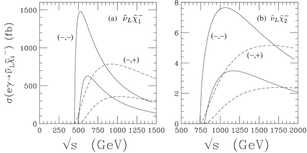
FIG. 2.: The upper two curves show the total cross section (in fb) for $e^{-}\gamma\to\tilde{\nu}\tilde{\chi}^{-}$ versus $\sqrt{s_{e\gamma}}$ (in GeV) for the SUSY and machine parameters given in the text: (a) $\tilde{\nu}\tilde{\chi}_{1}^{-}$; (b) $\tilde{\nu}\tilde{\chi}_{2}^{-}$. The solid curves represent $e$, $\gamma$ helicities $(-,-)$ and the dashed curves $(-,+)$. The lower two curves are corresponding results convoluted with the backscattered photon spectrum versus $\sqrt{s_{ee}}$.

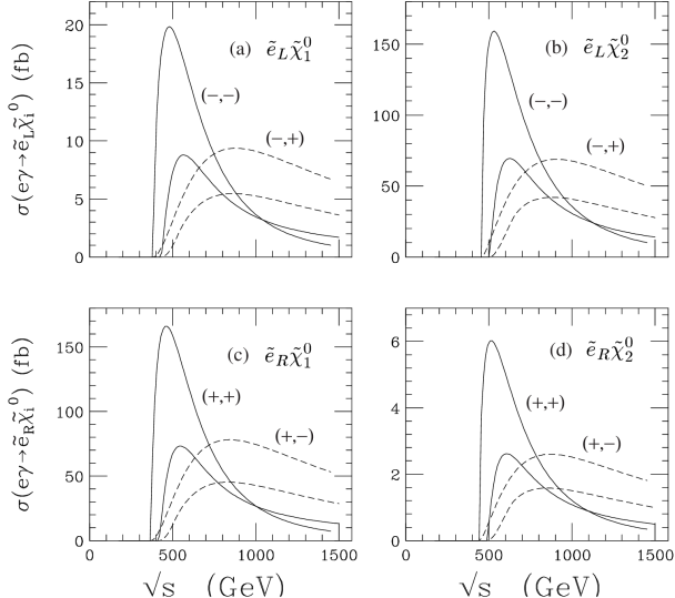
FIG. 3.: The upper two curves show the total cross section (in fb) for $e^{-}\gamma\to\tilde{e}\tilde{\chi}^{0}$ versus $\sqrt{s_{e\gamma}}$ (in GeV) for the SUSY and machine parameters given in the text: (a) $\tilde{e}_{L}\tilde{\chi}_{1}^{0}$; (b) $\tilde{e}_{L}\tilde{\chi}_{2}^{0}$; (c) $\tilde{e}_{R}\tilde{\chi}_{1}^{0}$; (d) $\tilde{e}_{R}\tilde{\chi}_{2}^{0}$. The solid curves represent $e$, $\gamma$ helicities $(-,-)$ for (a), (b) and $(+,+)$ for (c), (d). The dashed curves represent helicities $(-,+)$ for (a), (b) and $(+,-)$ for (c), (d). The lower two curves are corresponding results, convoluted with the backscattered photon spectrum, versus $\sqrt{s_{ee}}$.

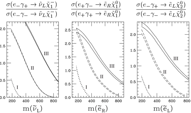
FIG. 4.: The ratio of total cross sections versus slepton mass (in GeV):
(a) $\sigma(e_{-}\gamma_{+}\to\tilde{\nu}_{L}\tilde{\chi}_{1}^{-})/\sigma(e_{-}\gamma_{-}\to\tilde{\nu}_{L}\tilde{\chi}_{1}^{-})$ vs $m_{\tilde{\nu}_{L}}$; (b) $\sigma(e_{+}\gamma_{-}\to\tilde{e}_{R}\tilde{\chi}_{1}^{0})/\sigma(e_{+}\gamma_{+}\to\tilde{e}_{R}\tilde{\chi}_{1}^{0})$ vs $m_{\tilde{e}_{R}}$; (c) $\sigma(e_{-}\gamma_{+}\to\tilde{e}_{L}\tilde{\chi}_{2}^{0})/\sigma(e_{-}\gamma_{-}\to\tilde{e}_{L}\tilde{\chi}_{2}^{0})$ vs $m_{\tilde{e}_{L}}$. Results for three colliders are presented: (I) $\sqrt{s_{ee}}=0.5$ TeV, ${\cal L}_{e\gamma}=25$ fb^-1; (II) $1$ TeV, $50$ fb^-1; (III) $1.5$ TeV, $100$ fb^-1. For each collider the upper and lower curves show the $\pm 1\sigma$ values for the ratio. The backscattered photon spectrum and the electron polarization are included in the calculations (see text).

REFERENCES

[1]
H. Murayama and M. E. Peskin, Ann. Rev. Nucl. Sci. 46, 533 (1996);
Physics and Technology of the Next Linear Collider, SLAC Report 485
(submitted to 1996 Snowmass Workshop);
ECFA/DESY Linear Collider Physics Working Group, hep-ph/9705442.
[2]
T. Tsukamota, K. Fujii, H. Murayama, M. Yamaguchi and
Y. Okada, Phys. Rev. D51, 3153 (1995);
J. Feng, M. E. Peskin, H. Murayama and X. Tata,
Phys. Rev. D52, 1418 (1995);
J. L. Feng and M. J. Strassler, Phys. Rev. D51, 4661 (1995).
[3] A. Bartl, H. Fraas and W. Majerotto, Z. Phys.
C30, 441 (1986).
[4]
H. Baer et al., Phys. Rev. D42, 2259 (1990);
D50, 4508 (1994);
I. Hinchliffe et al.,
Phys. Rev. D55, 5520 (1997).
[5]For recent comprehensive reviews and references,
see e.g. X. Tata, Proc. of the IX Jorge A. Swieca Summer School,
Campos do Jordão, Brazil (in press), hep-ph/9706307;
M. Drees, KEK-TH-501, hep-ph/9611409 (1996); S. P. Martin,
hep-ph/9709356.
[6]M. Dine and A. E. Nelson, Phys. Rev. D48, 1277 (1993);
M. Dine, A. E. Nelson and Y. Shirman, Phys. Rev. D51, 1362 (1995);
M. Dine, A. E. Nelson, Y. Nir and Y. Shirman, Phys. Rev. D53, 2658 (1996).
[7] H. Baer, C.-H. Chen, F. Paige and X. Tata,
Phys. Rev. D49, 3283 (1994).
[8]H.F. Ginzburg, G.L. Kotkin, V.G. Serbo and
V.I. Telnov,
Nucl. Inst. and Meth. 205, 47 (1983);
H.F. Ginzburg, G.L. Kotkin, S.L. Panfil, V.G. Serbo and V.I. Telnov,
Nucl. Inst. and Meth. 219, 5 (1984).
[9]V. Barger, M. S. Berger and P. Ohmann, Phys. Rev.
D47, 1093 (1993); Phys. Rev. D49, 4908 (1994);
V. Barger, M. S. Berger, P. Ohmann and R.J.N. Phillips,
Phys. Lett. B314, 351 (1993); P. Langacker and N. Polonsky,
Phys. Rev. D50, 2199 (1994); W. A. Bardeen, M. Carena,
S. Pokorski and C.E.M. Wagner, Phys. Lett. B320, 110
(1994); B. Schremp, Phys. Lett. B344, 193 (1995).
[10]Analyses of supergravity mass patterns include:
G. Ross and R. G. Roberts, Nucl. Phys. B377, 571 (1992);
R. Arnowitt and P. Nath, Phys. Rev. Lett. 69, 725 (1992);
M. Drees and M. M. Nojiri, Nucl. Phys. B369, 54 (1993);
S. Kelley, J. Lopez, D. Nanopoulos, H. Pois and K. Yuan,
Nucl. Phys. B398, 3 (1993); M. Olechowski and S. Pokorski,
Nucl. Phys. B404, 590 (1993); V. Barger, M. Berger and
P. Ohmann, Phys. Rev. D49, 4908, (1994); G. Kane,
C. Kolda, L. Roszkowski and J. Wells, Phys. Rev. D49, 6173
(1994); D. J. Castaño, E. Piard and P. Ramond, Phys. Rev.
D49, 4882, (1994); W. de Boer, R. Ehret and D. Kazakov,
Z. Phys. C67, 647 (1995); M. Noriji and X. Tata,
Phys. Rev. D50, 2148 (1994); H. Baer, C.-H. Chen, R. Munroe,
F. Paige and X. Tata, Phys. Rev. D51, 1046 (1995).
[11]See e.g. M. Drees and M. Nojiri, Phys. Rev.
D47, 376 (1993); R. G. Roberts and L. Roszkowski,
Phys. Lett. B309, 329 (1993).
[12] R. W. Robinett, Phys. Rev. D31, 1657 (1985).
[13] F. Cuypers, G.J. van Oldenberg, and R. Rückl,
Nucl. Phys. B383, 45 (1992); H.A. König and K.A. Peterson,
Phys. Lett. B294, 110 (1992); D.L. Borden, D. Bauer and D.O. Caldwell,
SLAC preprint SLAC-PUB-5715 (1992).
[14] T. Kon and A. Goto, Phys. Lett. B295, 324 (1992).
[15] D. Choudhury and F. Cuypers, Nucl. Phys.
B451, 16 (1995).
[16]
K. Kiers, J.N. Ng and G.H. Wu, Phys. Lett. B381, 177 (1996).
[17] H. Baer, F. Paige, S. Protpopescu, and X. Tata, in
Proceedings of the Workshop On Physics at Current Accelerators and
Supercolliders, eds. J. Hewitt, A. White and D. Zeppenfeld, Argonne
National Laboratory (1993).
[18] A. Ghosal, A. Kundu and B. Mukhopadhyaya,
Phys. Rev. D56, 504 (1997);
S. Ambrosanio, G. D. Kribs and S. P. Martin,
Phys. Rev. D56, 1761 (1997);
S. Dimopoulos, S. Thomas, and J.D. Wells, Nucl. Phys. B488, 39 (1997);
K.S Babu, C. Kolda, and F. Wilczek, Phys. Rev. Lett. 77, 3070 (1996).
[19] H. Baer, M. Brhlik, C. Chen, and X. Tata, Phys. Rev.
55, 4463 (1997).
[20]See e.g. S. Martin and P. Ramond, Phys. Rev.
D48, 5365 (1993).
[21]R. Arnowitt and P. Nath, hep-ph/9708451 (1997).