The Chiral-Odd Distribution Function $h_{1}$:
IR-Renormalon Contribution
and $\alpha_{s}$-Correction

M.Β Meyer-Hermann1, and A.Β SchΓ€fer2

1Institut fΓΌr Theoretische Physik, J.Β W.Β Goethe UniversitΓ€t Frankfurt,

PostfachΒ 11Β 19Β 32, D-60054Β Frankfurt am Main, Germany

2FakultΓ€t Physik, UniversitΓ€t Regensburg, D-93040Β Regensburg, Germany

Abstract: The chiral-odd distribution function $h_{1}$ is discussed in the framework of the renormalon approach. Using a bag-model calculation for $h_{1}$, we calculate its intrinsic uncertainty due to renormalon poles. The result is given as a function of Bjorken-$x$ as well as for the first moments separately. We also extract the perturbative corrections to the first moments of $h_{1}$.

1 Introduction

While in totally inclusive deep inelastic scattering (DIS) the quark chirality is conserved up to terms proportional to the quark masses, this is not the case in the Drell-Yan process. Here a quark-antiquark-pair is annihilated to a virtual photon, so that in the cross-section the quarks originating and ending in the same nucleon may carry different chirality. This gives raise to chiral odd distribution functions, which first appeared in the discussion of the transverse polarized Drell-Yan process [1]. This chiral odd distribution function is defined by a twist-2 operator and is called the transversity distribution $h_{1}$. Unlike the helicity asymmetry $g_{1}$, $h_{1}$ has no partonic interpretation in the chiral basis. Changing to the transversity basis [2] $g_{1}$ looses its partonic interpretation and $h_{1}$ gets one instead. It is interpreted as the probability to find a quark in a transversely polarized nucleon in an eigenstate of the transverse Pauli-Lubanski vector with eigenvalue $+1/2$, minus the same with eigenvalue $-1/2$.

Some experiments are planned to measure $h_{1}$ in the near future, especially at RHIC (BNL) and possibly by the COMPASS experiment at CERN β€” for a general review of the possibilities for measuring the transversity distribution see [3] β€”, so that there is need for theoretical predictions for $h_{1}$. The anomalous dimension which we will also consider in this contribution was calculated in [4]. In the nonrelativistic quark models $g_{1}$ and $h_{1}$ are identical. The positivity of parton probabilities implies the inequality $\left|h_{1}(x)\right|\leq f_{1}(x)$ and the Soffer inequality [5] $2\left|h_{1}(x)\right|\leq f_{1}(x)+g_{1}(x)$. A bag model calculation predict $\left|h_{1}(x)\right|\geq\left|g_{1}(x)\right|$, which may be correct in general [6]. For medium large Bjorken-$x$ there exists a QCD-sum rule calculation [7], predicting a much smaller value for $h_{1}$ than the already mentioned bag model calculation.

We wish to contribute to this theoretical discussion by calculating an intrinsic uncertainty of the perturbative series due to IR-renormalon poles. This uncertainty is a systematic error for the experimental measurement of $h_{1}$. In addition we discuss the anomalous dimension in the one loop approximaion and extract the $\alpha_{s}$ correction to the first moments of the transversity distribution.

2 Definitions

2.1 Forward-Scattering-Amplitude

The definition of $h_{1}$ in terms of an operator matrix element reads [1, 6, 7]:

i2β€‹βˆ«d​y+2​π​ei​y+​x​<p,s|ΟˆΒ―β€‹(0)​σμ​ν​γ5β€‹Οˆβ€‹(y+​n)|p,s>𝑖2𝑑subscript𝑦2πœ‹superscript𝑒𝑖subscript𝑦π‘₯quantum-operator-productπ‘π‘ Β―πœ“0subscriptπœŽπœ‡πœˆsubscript𝛾5πœ“subscript𝑦𝑛𝑝𝑠\displaystyle\frac{i}{2}\int\frac{dy_{+}}{2\pi}\,e^{iy_{+}x}\big{<}p,s\big{|}\overline{\psi}(0)\sigma_{\mu\nu}\gamma_{5}\psi(y_{+}n)\big{|}p,s\big{>} $\displaystyle=$ $\displaystyle h_{1}(x,q^{2})\left(s_{\bot\mu}p_{\nu}-s_{\bot\nu}p_{\mu}\right)$
+hL​(x,q2)​m2​(pμ​nΞ½βˆ’pν​nΞΌ)​(sβ‹…n)subscriptβ„ŽπΏπ‘₯superscriptπ‘ž2superscriptπ‘š2subscriptπ‘πœ‡subscriptπ‘›πœˆsubscriptπ‘πœˆsubscriptπ‘›πœ‡β‹…π‘ π‘›\displaystyle+\,h_{L}(x,q^{2})m^{2}\left(p_{\mu}n_{\nu}-p_{\nu}n_{\mu}\right)(s\cdot n) $\displaystyle+$ $\displaystyle h_{3}(x,q^{2})m^{2}\left(s_{\bot\mu}n_{\nu}-s_{\bot\nu}n_{\mu}\right)$ (1)

where $x=-q^{2}/(2p\cdot q)$ is the Bjorken variable, $n^{\nu}$ is a light cone vector with $n^{2}=0$ of dimension (m​a​s​s)βˆ’1superscriptπ‘šπ‘Žπ‘ π‘ 1(mass)^{-1}, $p$ is the proton momentum and $s$ is the proton spin. $p^{2}=m^{2}$, $s^{2}=-1$ and $p\cdot s=0$. $p\cdot n=1$ and the transverse part of the spin vector is defined by the decomposition sΞΌ=(sβ‹…n)​pΞΌ+(sβ‹…p)​nΞΌ+sβŠ₯ΞΌsubscriptπ‘ πœ‡β‹…π‘ π‘›subscriptπ‘πœ‡β‹…π‘ π‘subscriptπ‘›πœ‡subscript𝑠bottomπœ‡s_{\mu}=(s\cdot n)p_{\mu}+(s\cdot p)n_{\mu}+s_{\bot\mu}. The contraction of this expression with the light cone vector $n^{\nu}$ gives:

i2β€‹βˆ«d​y+2​π​ei​y+​x​<p,s|ΟˆΒ―β€‹(0)​σμ​ν​nν​γ5β€‹Οˆβ€‹(y+​n)|p,s>=h1​(x,q2)​sβŠ₯ΞΌβˆ’hL​(x,q2)​m2​nμ​(sβ‹…n).𝑖2𝑑subscript𝑦2πœ‹superscript𝑒𝑖subscript𝑦π‘₯quantum-operator-productπ‘π‘ Β―πœ“0subscriptπœŽπœ‡πœˆsuperscriptπ‘›πœˆsubscript𝛾5πœ“subscript𝑦𝑛𝑝𝑠subscriptβ„Ž1π‘₯superscriptπ‘ž2subscript𝑠bottomπœ‡subscriptβ„ŽπΏπ‘₯superscriptπ‘ž2superscriptπ‘š2subscriptπ‘›πœ‡β‹…π‘ π‘›\frac{i}{2}\int\frac{dy_{+}}{2\pi}\,e^{iy_{+}x}\big{<}p,s\big{|}\overline{\psi}(0)\sigma_{\mu\nu}n^{\nu}\gamma_{5}\psi(y_{+}n)\big{|}p,s\big{>}\;=\;h_{1}(x,q^{2})s_{\bot\mu}-h_{L}(x,q^{2})m^{2}n_{\mu}(s\cdot n)\quad. (2)

It is possible to relate the transversity distribution $h_{1}$ to the imaginary part of the forward scattering amplitude on the leading twist-level [7]:

$$T_{\mu}\;=\;\frac{i}{2}\int d^{4}y\,e^{iqy}\big{<}p,s\big{|}T\left(j_{\mu 5}(y)j_{S}(0)+j_{S}(y)j_{\mu 5}(0)\right)\big{|}p,s\big{>}\quad.$$ (3)

Here $j_{\mu 5}(y)=\overline{\psi}(y)\gamma_{\mu}\gamma_{5}\psi(y)$ is a axial-vector current, $j_{S}(y)=\overline{\psi}(y)\psi(y)$ is a scalar current and $T$ denotes the time-ordered product. Summation over flavor indices is assumed. Equivalently one may use a time-ordered product of a vector-current $j_{\mu}(y)=\overline{\psi}(y)\gamma_{\mu}\psi(y)$ and a pseudoscalar current $j_{5}(y)=\overline{\psi}(y)\gamma_{5}\psi(y)$.

To prove the relation between this definition and the operator-definition Eq. (2.1) of the transversity distribution, one has to decompose the forward scattering amplitude into its Lorentz-structures using the conservation of either the axial-vector or the vector current. The conservation of the axial-vector current is correct only for the flavor nonsinglet current, so that the proof remains correct up to an order $\alpha_{s}$-correction only. As the vector-current is conserved independently of the flavor combination under consideration we prefer the definition

$$T_{\mu}\;=\;\frac{i}{2}\int d^{4}y\,e^{iqy}\big{<}p,s\big{|}T\left(j_{\mu}(y)j_{5}(0)+j_{5}(y)j_{\mu}(0)\right)\big{|}p,s\big{>}\quad.$$ (4)

To find the realation to $h_{1}$ the current product has to be expanded collecting the terms with one incoming quark, one outgoing quark and one quark propagator $S(y)=i\not\!\partial\,\Delta(y)$, where $\Delta$ is the Pauli-Jordan function. The Pauli-Jordan function is expanded on the light cone and only the leading term is taken into account. The imaginary part of the s-channel-term of the forward scattering amplitude takes the form:

$\displaystyle{\rm Im}\,T_{\mu}$ $\displaystyle=$ βˆ’12β€‹Ο€β€‹βˆ«d4​y​ei​q​y​<p,s|:ΟˆΒ―β€‹(y)​σμ​ν​yν​i​γ5β€‹Οˆβ€‹(0):|p,s>​δ′​(y2):12πœ‹superscript𝑑4𝑦superscriptπ‘’π‘–π‘žπ‘¦braπ‘π‘ Β―πœ“π‘¦subscriptπœŽπœ‡πœˆsuperscriptπ‘¦πœˆπ‘–subscript𝛾5πœ“0:ket𝑝𝑠superscript𝛿′superscript𝑦2\displaystyle-\frac{1}{2\pi}\int d^{4}y\,e^{iqy}\big{<}p,s\big{|}:\overline{\psi}(y)\sigma_{\mu\nu}y^{\nu}i\gamma_{5}\psi(0):\big{|}p,s\big{>}\delta^{\prime}(y^{2}) (5)
+12β€‹Ο€β€‹βˆ«d4​y​ei​q​y​<p,s|:ΟˆΒ―β€‹(0)​σμ​ν​yν​i​γ5β€‹Οˆβ€‹(y):|p,s>​δ′​(y2).:12πœ‹superscript𝑑4𝑦superscriptπ‘’π‘–π‘žπ‘¦braπ‘π‘ Β―πœ“0subscriptπœŽπœ‡πœˆsuperscriptπ‘¦πœˆπ‘–subscript𝛾5πœ“π‘¦:ket𝑝𝑠superscript𝛿′superscript𝑦2\displaystyle+\frac{1}{2\pi}\int d^{4}y\,e^{iqy}\big{<}p,s\big{|}:\overline{\psi}(0)\sigma_{\mu\nu}y^{\nu}i\gamma_{5}\psi(y):\big{|}p,s\big{>}\delta^{\prime}(y^{2})\quad.

Here $\sigma_{\mu\nu}=\frac{i}{2}\left[\gamma_{\mu},\gamma_{\nu}\right]$ and $\delta^{\prime}(y^{2})=\left(\partial/\partial(y^{2})\right)\delta(y^{2})$. Substituting light cone variables $y_{-}=y_{0}-y_{3}$ and $2y_{+}=y_{0}+y_{3}$, integrating by parts, using translation invariance, and putting this expression on the light cone by choosing $y$ such that $y^{2}=0$, one gets

$\displaystyle{\rm Im}\,T_{\mu}$ $\displaystyle=$ βˆ’i2β€‹βˆ«d​y+2​ei​y+​x​<p,s|:ΟˆΒ―β€‹(0)​σμ​ν​nν​γ5β€‹Οˆβ€‹(y+​n):|p,s>.:𝑖2𝑑subscript𝑦2superscript𝑒𝑖subscript𝑦π‘₯braπ‘π‘ Β―πœ“0subscriptπœŽπœ‡πœˆsuperscriptπ‘›πœˆsubscript𝛾5πœ“subscript𝑦𝑛:ket𝑝𝑠\displaystyle-\frac{i}{2}\int\frac{dy_{+}}{2}\,e^{iy_{+}x}\big{<}p,s\big{|}:\overline{\psi}(0)\sigma_{\mu\nu}n^{\nu}\gamma_{5}\psi(y_{+}n):\big{|}p,s\big{>}\quad. (6)

This result has the form of Eq. (2), so that one gets a relation between the s-channel-part of the forward scattering amplitude and the transversity distribution by collecting the terms proportional to $s_{\bot\mu}$:

$$h_{1}(x)s_{\bot\mu}\;=\;\frac{1}{\pi}\,\left.{\rm Im}\,T_{\mu}\right|_{s_{\bot\mu}}\quad.$$ (7)

2.2 Light Cone Expansion and Moments

The light cone expansion of the forward scattering amplitude may be writen as:

$$\left.T_{\mu}\right|_{s_{\bot\mu}}\;=\;2s_{\bot\mu}\sum_{m=0}^{\infty}C_{m}\left(\frac{Q^{2}}{\mu^{2}},\alpha_{s}\right)A_{m}(\mu^{2})\,\omega^{m+1}+{\rm higher\,twist}$$ (8)

where $\omega=1/x$. $A_{m}$ are the reduced matrix elements of the local twist-2 operators relevant for $h_{1}$:

$$\big{<}p,s\big{|}\overline{\psi}\sigma^{\lambda\{\rho}i\gamma_{5}iD^{\mu_{1}}\cdots iD^{\mu_{m}\}}\psi\big{|}p,s\big{>}\;=\;2A_{m}(s^{\lambda}p^{\{\rho}-p^{\lambda}s^{\{\rho})p^{\mu_{1}}\cdots p^{\mu_{m}\}}\psi-{\rm traces}\quad.$$ (9)

The brackets denote total symmetrization of all included indices. The symmetrization and the subtraction of the traces are necessary to extract the leading twist part of the matrix element. The moments of $h_{1}$ have to be defined as $M_{m}=C_{m}A_{m}$ to get the general expression:

$$2s_{\bot\mu}M_{n}\;=\;\frac{1}{\pi}\int_{0}^{1}dx\,x^{n}\left.\left(Im\,T_{\mu}(x)+(-)^{n}Im\,T_{\mu}(-x)\right)\right|_{s_{\bot\mu}}\quad.$$ (10)

Using Eq. (7) the moments become:

$$M_{n}\;=\;\frac{1}{2}\int_{0}^{1}dx\,x^{n}\left(h_{1}(x)+(-)^{n}h_{1}(-x)\right)$$ (11)

for $n=0,1,\ldots$ This result coincides with the expression found by Jaffe and Ji [6].

The operators in Eq. (9) have a well defined behaviour under charge conjugation: they are $C$-odd for even $n$ and $C$-even for odd $n$. This change in sign corresponds to the relative sign of $h_{1}(x)$ and $h_{1}(-x)$ in the moments Eq. (11). To obtain the correct relation between the antiquark and the quark transversity distribution one may look at the first moment:

$$M_{0}\;=\;\frac{1}{2}\int_{0}^{1}dx\,\left(h_{1}(x)+h_{1}(-x)\right)\quad.$$ (12)

As this expression is odd under charge conjugation, the antiquark transversity distribution should be $\overline{h}_{1}(x)=-h_{1}(-x)$. It follows that the contributions of sea quarks cancel for even moments in general and only the valence quarks contribute, while the sea quark contributions add for odd moments.

3 Renomalon ambiguity of $h_{1}$

We are calculating the IR-renormalon contribution [8] to the structure function defined by Eq. (3) and (7). As its twist-2 part is related to the transversity distribution $h_{1}$, the IR-renormalon contribution may be interpreted as intrinsic ambiguity of the perturbative expansion to $h_{1}$. Perturbative series in QCD are asymptotic ones, implying that the radiative corrections of higher and higher orders get smaller only up to a finite order $m_{0}$ and diverge for larger orders in $\alpha_{s}$. The uncertainty of the series is of the order of the smallest contribution and has the form of a power correction [9], so that the QCD perturbative series on the lowest twist level may be written as (as=Ξ±s/(4​π)subscriptπ‘Žπ‘ subscript𝛼𝑠4πœ‹a_{s}=\alpha_{s}/(4\pi)):

Cn​(Q2=ΞΌ2,as)=βˆ‘k=0m0Bn(k)​ask+Cn(1)​ΛC2​eβˆ’CQ2+Cn(2)​ΛC4​eβˆ’2​CQ4+π’ͺ​(1Q6).subscript𝐢𝑛superscript𝑄2superscriptπœ‡2subscriptπ‘Žπ‘ superscriptsubscriptπ‘˜0subscriptπ‘š0superscriptsubscriptπ΅π‘›π‘˜superscriptsubscriptπ‘Žπ‘ π‘˜superscriptsubscript𝐢𝑛1superscriptsubscriptΛ𝐢2superscript𝑒𝐢superscript𝑄2superscriptsubscript𝐢𝑛2superscriptsubscriptΛ𝐢4superscript𝑒2𝐢superscript𝑄4π’ͺ1superscript𝑄6C_{n}\left(Q^{2}=\mu^{2},a_{s}\right)\;=\;\sum_{k=0}^{m_{0}}B_{n}^{(k)}a_{s}^{k}+C_{n}^{(1)}\frac{\Lambda_{C}^{2}e^{-C}}{Q^{2}}+C_{n}^{(2)}\frac{\Lambda_{C}^{4}e^{-2C}}{Q^{4}}+{\cal O}\left(\frac{1}{Q^{6}}\right)\quad. (13)

Note that the $1/Q$ term is not present in the above expression. It was shown for Drell-Yan on the one gluon exchange level that these corrections are cancelled by higher order perturbative contributions [10] and that the $1/Q^{2}$-term is the leading power correction. The uncertainty may be determined by the exact calculation of the perturbative corrections up to the order $m_{0}(Q^{2})$, which is a very demanding procedure.

Instead we calculate the forward scattering amplitude Eq. (3) on the one gluon exchange level, using a Borel transformed effective gluon propagator [11]:

ℬ1/as​[as​Dμ​νa​b​(k)]​(u)=Ξ΄a​b​gΞΌβ€‹Ξ½βˆ’kμ​kΞ½k2k2​(ΞΌ2​eβˆ’Cβˆ’k2)Ξ²0​u.subscriptℬ1subscriptπ‘Žπ‘ delimited-[]subscriptπ‘Žπ‘ subscriptsuperscriptπ·π‘Žπ‘πœ‡πœˆπ‘˜π‘’superscriptπ›Ώπ‘Žπ‘subscriptπ‘”πœ‡πœˆsubscriptπ‘˜πœ‡subscriptπ‘˜πœˆsuperscriptπ‘˜2superscriptπ‘˜2superscriptsuperscriptπœ‡2superscript𝑒𝐢superscriptπ‘˜2subscript𝛽0𝑒{\cal B}_{1/a_{s}}[a_{s}D^{ab}_{\mu\nu}(k)](u)\;=\;\delta^{ab}\frac{g_{\mu\nu}-\frac{k_{\mu}k_{\nu}}{k^{2}}}{k^{2}}\left(\frac{\mu^{2}e^{-C}}{-k^{2}}\right)^{\beta_{0}u}\quad. (14)

$C$ corrects for the renormalization scheme dependence ($C=-\frac{5}{3}$ for $\overline{MS}$-scheme), $\mu$ is the renormalization scale, and $u$ is the Borel parameter. The effective gluon propagator is constructed by replacing the coupling assubscriptπ‘Žπ‘ a_{s} by the running coupling constant, that is by a resummation of all quark- and gluon-loop insertions in one gluon-propagator. In the first order of assubscriptπ‘Žπ‘ a_{s} this propagator leads to exact results. Looking at higher order corrections the restriction on one exchanged effective gluon corresponds to the large $N_{f}$-limit [12], where $N_{f}$ denotes the number of quark flavors. The next-to-leading $N_{f}$-terms are approximated by naive-nonabelianization (NNA) [13]. This corresponds to the replacement of the one loop QED-beta-function by the QCD-beta-function $\beta_{0}=11-\frac{2}{3}N_{f}$ or equivalently to $N_{f}\rightarrow N_{f}-\frac{33}{2}$. The quality of this approximation has been checked [14, 15] for the unpolarized structure functions $F_{2}$ and $F_{L}$ and for the polarized structure function $g_{1}$ by comparing the NNA perturbative coefficients with the known exact ones. This comparison gave very reasonable results for $F_{L}$ and $g_{1}$, while the results for $F_{2}$ are less convincing.

Formally, asymptotic freedom is destroyed in the large $N_{f}$-limit. One should recognize that the large $N_{f}$-limit is used to select graphs and has to be understood as a definition of an approximation procedure. At the end $N_{f}$ will be set to 4, so that $\beta_{0}$ stays in an asymptotic free region. This procedure is technically analogous to the use of the large $N_{c}$-limit [16], even if the physical content is different.

In the Borel plane the ambiguity of the truncated perturbative series in Eq. (13) is reflected in IR-renormalon poles, which hinder an unambigous inverse Borel transformation. This ambiguity of the perturbative series may be interpreted as twist-4 contribution of the structure function defined by Eq. (3) and (7). Such estimations of higher twist corrections gave very reasonable results [17, 18, 14, 15]. However the transversity distribution is defined by pure twist-2 operators and the relation of Eq. (3) to the operator definition of the transversity distribution Eq. (2.1) was shown for the twist-2 part of the structure function only. This means that the IR-renormalon ambiguity of the structure function has to be interpreted as intrinsic uncertainty of the perturbative expansion of the transversity distribution $h_{1}$.

So let us calculate the Borel-transformed s-channel forward scattering amplitude $T_{\mu}$ in Eq. (3) on the one gluon exchange level using the effective gluon propagator Eq. (14). The result is a series in $\omega=1/x$ which has to be compared with Eq. (8)

ℬ1as​(TΞΌ)|sβŠ₯ΞΌ=sβŠ₯ΞΌβ€‹βˆ‘m=0βˆžβ„¬1as​(Cm​(Q2ΞΌ2,as))​Am​(ΞΌ2)​ωm+1+higher​twistevaluated-atsubscriptℬ1subscriptπ‘Žπ‘ subscriptπ‘‡πœ‡subscript𝑠bottomπœ‡subscript𝑠bottomπœ‡superscriptsubscriptπ‘š0subscriptℬ1subscriptπ‘Žπ‘ subscriptπΆπ‘šsuperscript𝑄2superscriptπœ‡2subscriptπ‘Žπ‘ subscriptπ΄π‘šsuperscriptπœ‡2superscriptπœ”π‘š1highertwist\left.{\cal B}_{\frac{1}{a_{s}}}\left(T_{\mu}\right)\right|_{s_{\bot\mu}}\;=\;s_{\bot\mu}\sum_{m=0}^{\infty}{\cal B}_{\frac{1}{a_{s}}}\left(C_{m}\left(\frac{Q^{2}}{\mu^{2}},a_{s}\right)\right)A_{m}(\mu^{2})\,\omega^{m+1}+{\rm higher\,twist} (15)

where the reduced matrix element was determined at the tree level to be $A_{n}=1$ and a factor $2$ is missing because the exchange graphs are not included in this expression due to the restriction on the s-channel contribution. We obtain for the Borel transformed Wilson coefficient:

ℬ1as​[Cn​(Q2ΞΌ2,as)]​(s)=CF​(ΞΌ2​eβˆ’CQ2)ssubscriptℬ1subscriptπ‘Žπ‘ delimited-[]subscript𝐢𝑛superscript𝑄2superscriptπœ‡2subscriptπ‘Žπ‘ π‘ subscript𝐢𝐹superscriptsuperscriptπœ‡2superscript𝑒𝐢superscript𝑄2𝑠\displaystyle{\cal B}_{\frac{1}{a_{s}}}\left[C_{n}\left(\frac{Q^{2}}{\mu^{2}},a_{s}\right)\right](s)\;=\;C_{F}\left(\frac{\mu^{2}e^{-C}}{Q^{2}}\right)^{s}
$\displaystyle\Bigg{\{}\frac{1}{s}\left[\frac{5}{1+s}-\frac{\Gamma(1+s+n)}{\Gamma(1+s)\Gamma(1+n)}+\sum_{k=1}^{n}\frac{\Gamma(s+k)}{\Gamma(1+s)\Gamma(1+k)}\frac{4k}{1+s+k}\right]$
+11βˆ’s​[41+sβˆ’2​Γ​(1+s+n)Γ​(1+s)​Γ​(1+n)+βˆ‘k=1nΓ​(s+k)Γ​(1+s)​Γ​(1+k)​4​(1+k)1+s+k]11𝑠delimited-[]41𝑠2Ξ“1𝑠𝑛Γ1𝑠Γ1𝑛superscriptsubscriptπ‘˜1π‘›Ξ“π‘ π‘˜Ξ“1𝑠Γ1π‘˜41π‘˜1π‘ π‘˜\displaystyle+\frac{1}{1-s}\left[\frac{4}{1+s}-\frac{2\Gamma(1+s+n)}{\Gamma(1+s)\Gamma(1+n)}+\sum_{k=1}^{n}\frac{\Gamma(s+k)}{\Gamma(1+s)\Gamma(1+k)}\frac{4(1+k)}{1+s+k}\right]
$\displaystyle+\frac{1}{2-s}\left[\frac{1}{1+s}+\frac{\Gamma(1+s+n)}{\Gamma(1+s)\Gamma(1+n)}+\sum_{k=1}^{n}\frac{\Gamma(s+k)}{\Gamma(1+s)\Gamma(1+k)}\frac{2}{1+s+k}\right]\Bigg{\}}$ (16)

where $s=\beta_{0}u$ replaces the Borel parameter $u$. We find IR-renormalon poles at $s=0,1,2$, as usual for DIS. This is not a general statement as in the case of $e^{+}e^{-}$-fragmentation one obtains an infinite sum of poles with even powers of $1/Q$ [17]. The Wilson coefficient has still to be renormalized and the coefficient of the $1/s$-pole should give the anomalous dimension as will be discussed in the next section.

In the Borel-plane the ambiguity $C_{n}^{(k)}$ of the perturbative series in Eq. (13) can be rediscovered as ambiguity of the inverse Borel transformation due to the IR-renormalon poles or in other words as the imaginary part of the Laplace integral:

βˆ‘kCn(k)​(Ξ›C2​eβˆ’CQ2)k=1π​β0​Imβ€‹βˆ«0βˆžπ‘‘s​eβˆ’s/(Ξ²0​as)​ℬ1as​[Cn​(Q2ΞΌ2,as)]​(s).subscriptπ‘˜superscriptsubscriptπΆπ‘›π‘˜superscriptsuperscriptsubscriptΛ𝐢2superscript𝑒𝐢superscript𝑄2π‘˜1πœ‹subscript𝛽0Imsuperscriptsubscript0differential-d𝑠superscript𝑒𝑠subscript𝛽0subscriptπ‘Žπ‘ subscriptℬ1subscriptπ‘Žπ‘ delimited-[]subscript𝐢𝑛superscript𝑄2superscriptπœ‡2subscriptπ‘Žπ‘ π‘ \sum_{k}C_{n}^{(k)}\left(\frac{\Lambda_{C}^{2}e^{-C}}{Q^{2}}\right)^{k}\;=\;\frac{1}{\pi\beta_{0}}{\rm Im}\int_{0}^{\infty}ds\;e^{-s/(\beta_{0}a_{s})}{\cal B}_{\frac{1}{a_{s}}}\left[C_{n}\left(\frac{Q^{2}}{\mu^{2}},a_{s}\right)\right](s)\quad. (17)

We get

$\displaystyle C_{n}^{(1)}$ $\displaystyle=$ $\displaystyle\pm\frac{2C_{F}}{\beta_{0}}\left(3+n-\frac{2}{1+n}-\frac{2}{2+n}-2\sum_{k=1}^{n}\frac{1}{k}\right)$
$\displaystyle C_{n}^{(2)}$ $\displaystyle=$ $\displaystyle\pm\frac{C_{F}}{\beta_{0}}\left(3+\frac{1}{2}(1+n)(4+n)-\frac{2}{1+n}-\frac{2}{2+n}-\frac{2}{3+n}-2\sum_{k=1}^{n}\frac{1}{k}\right)\quad.$ (18)

The signs of these twist-2 uncertainty terms remain undetermined, because it is not clear in which way the pole should be circumvented in the Laplace integral.

The ambiguity of the Laplace integral is an intrinsic uncertainty of the twist-2 transversity distribution. The ratio of the moments of this uncertainty $h_{1}^{IR}$ and the moments of $h_{1}$ is expanded up to the order as/Q2subscriptπ‘Žπ‘ superscript𝑄2a_{s}/Q^{2}

$\displaystyle M_{n}^{\rm IR}$ $\displaystyle=$ Cn(1)​Λ2​eβˆ’CQ2+π’ͺ​(asQ2,1Q4)βˆ‘k=0m0Bn(k)​ask+Cn(1)​Λ2​eβˆ’CQ2+π’ͺ​(asQ2,1Q4)​Mnsuperscriptsubscript𝐢𝑛1superscriptΞ›2superscript𝑒𝐢superscript𝑄2π’ͺsubscriptπ‘Žπ‘ superscript𝑄21superscript𝑄4superscriptsubscriptπ‘˜0subscriptπ‘š0superscriptsubscriptπ΅π‘›π‘˜superscriptsubscriptπ‘Žπ‘ π‘˜superscriptsubscript𝐢𝑛1superscriptΞ›2superscript𝑒𝐢superscript𝑄2π’ͺsubscriptπ‘Žπ‘ superscript𝑄21superscript𝑄4subscript𝑀𝑛\displaystyle\frac{C_{n}^{(1)}\frac{\Lambda^{2}e^{-C}}{Q^{2}}+{\cal O}\left(\frac{a_{s}}{Q^{2}},\frac{1}{Q^{4}}\right)}{\sum_{k=0}^{m_{0}}B_{n}^{(k)}a_{s}^{k}+C_{n}^{(1)}\frac{\Lambda^{2}e^{-C}}{Q^{2}}+{\cal O}\left(\frac{a_{s}}{Q^{2}},\frac{1}{Q^{4}}\right)}\,M_{n} (19)
$\displaystyle\approx$ [Cn(1)Bn(0)​Λ2​eβˆ’CQ2+π’ͺ​(asQ2,1Q4)]​Mn.delimited-[]superscriptsubscript𝐢𝑛1superscriptsubscript𝐡𝑛0superscriptΞ›2superscript𝑒𝐢superscript𝑄2π’ͺsubscriptπ‘Žπ‘ superscript𝑄21superscript𝑄4subscript𝑀𝑛\displaystyle\left[\frac{C_{n}^{(1)}}{B_{n}^{(0)}}\frac{\Lambda^{2}e^{-C}}{Q^{2}}+{\cal O}\left(\frac{a_{s}}{Q^{2}},\frac{1}{Q^{4}}\right)\right]M_{n}\quad.

Here the truncated perturbative series Eq. (13) was used for the moments of $h_{1}$. The lowest order twist-2 perturbative coefficient $B_{n}^{(0)}$ is determined by the tree-graph and is 1. As an illustration we will insert for $M_{n}$ a theoretical model prediction for the transversity distribution.

ΒΏFrom Eq. (3) and (19) we can calculate the IR-renormalon uncertainty $U_{n}$ for each moment, where

∫01𝑑x​xn​(h1​(x)βˆ’(βˆ’)n​hΒ―1​(x))=An(0)​(1Β±Un)+π’ͺ​(as),superscriptsubscript01differential-dπ‘₯superscriptπ‘₯𝑛subscriptβ„Ž1π‘₯superscript𝑛subscriptΒ―β„Ž1π‘₯superscriptsubscript𝐴𝑛0plus-or-minus1subscriptπ‘ˆπ‘›π’ͺsubscriptπ‘Žπ‘ \int_{0}^{1}dx\,x^{n}\left(h_{1}(x)-(-)^{n}\overline{h}_{1}(x)\right)\;=\;A_{n}^{(0)}\left(1\pm U_{n}\right)+{\cal O}(a_{s})\quad, (20)

where $A_{n}^{(0)}$ denotes the leading contribution to the moments. At $Q^{2}=4\,{\rm GeV}^{2}$ and with $\Lambda_{\overline{MS}}=200\,{\rm MeV}$, $N_{f}=4$, $C_{F}=\frac{4}{3}$ and $\beta_{0}=11-\frac{2}{3}N_{f}$ we find:

∫01𝑑x​(h1​(x)βˆ’hΒ―1​(x))=A0(0)+π’ͺ​(as),superscriptsubscript01differential-dπ‘₯subscriptβ„Ž1π‘₯subscriptΒ―β„Ž1π‘₯superscriptsubscript𝐴00π’ͺsubscriptπ‘Žπ‘ \displaystyle\int_{0}^{1}dx\,\left(h_{1}(x)-\overline{h}_{1}(x)\right)\;=\;A_{0}^{(0)}+{\cal O}(a_{s})\quad,
∫01𝑑x​x​(h1​(x)+hΒ―1​(x))=A1(0)​(1Β±0.0057)+π’ͺ​(as),superscriptsubscript01differential-dπ‘₯π‘₯subscriptβ„Ž1π‘₯subscriptΒ―β„Ž1π‘₯superscriptsubscript𝐴10plus-or-minus10.0057π’ͺsubscriptπ‘Žπ‘ \displaystyle\int_{0}^{1}dx\,x\left(h_{1}(x)+\overline{h}_{1}(x)\right)\;=\;A_{1}^{(0)}(1\pm 0.0057)+{\cal O}(a_{s})\quad,
∫01𝑑x​x2​(h1​(x)βˆ’hΒ―1​(x))=A2(0)​(1Β±0.014)+π’ͺ​(as),superscriptsubscript01differential-dπ‘₯superscriptπ‘₯2subscriptβ„Ž1π‘₯subscriptΒ―β„Ž1π‘₯superscriptsubscript𝐴20plus-or-minus10.014π’ͺsubscriptπ‘Žπ‘ \displaystyle\int_{0}^{1}dx\,x^{2}\left(h_{1}(x)-\overline{h}_{1}(x)\right)\;=\;A_{2}^{(0)}(1\pm 0.014)+{\cal O}(a_{s})\quad,
∫01𝑑x​x3​(h1​(x)+hΒ―1​(x))=A3(0)​(1Β±0.024)+π’ͺ​(as),superscriptsubscript01differential-dπ‘₯superscriptπ‘₯3subscriptβ„Ž1π‘₯subscriptΒ―β„Ž1π‘₯superscriptsubscript𝐴30plus-or-minus10.024π’ͺsubscriptπ‘Žπ‘ \displaystyle\int_{0}^{1}dx\,x^{3}\left(h_{1}(x)+\overline{h}_{1}(x)\right)\;=\;A_{3}^{(0)}(1\pm 0.024)+{\cal O}(a_{s})\quad,
∫01𝑑x​x4​(h1​(x)βˆ’hΒ―1​(x))=A4(0)​(1Β±0.036)+π’ͺ​(as).superscriptsubscript01differential-dπ‘₯superscriptπ‘₯4subscriptβ„Ž1π‘₯subscriptΒ―β„Ž1π‘₯superscriptsubscript𝐴40plus-or-minus10.036π’ͺsubscriptπ‘Žπ‘ \displaystyle\int_{0}^{1}dx\,x^{4}\left(h_{1}(x)-\overline{h}_{1}(x)\right)\;=\;A_{4}^{(0)}(1\pm 0.036)+{\cal O}(a_{s})\quad. (21)

We get no IR-renormalon uncertainty for the first moment. The IR-renormalon uncertainty becomes larger for higher moments, so that we expect larger ambiguities of the transversity distribution in the region of larger Bjorken-$x$. For higher moments the contribution of $\overline{h}_{1}$ can be considered as marginal, so that the above ambiguities should remain approximately correct for $\int_{0}^{1}dxx^{n}h_{1}(x)$ with $n>2$. This is of course not the case for the first and the second moment ($n=1$). A rough estimate gives rise to a sea-quark effect of the same order as the calculated uncertainty.

Refer to caption


Figure 1: The bag model calculation [6] for $h_{1}-\overline{h}_{1}$ (full line) and the IR-renormalon ambiguity evaluated at $Q^{2}=4\,{\rm GeV}^{2}$ multiplied by a factor of $10$ (dotted line). There are two changes in sign at $x\approx 0.25$ and $x\approx 0.4$. The ambiguity was added and subtracted from the bag model calculation (dashed lines), ($\Lambda_{\overline{MS}}=200~{}{\rm MeV}$, and $N_{f}=4$).

Refer to caption

Figure 2: The relative magnitude of the IR-renormalon ambiguity with respect to the bag model calculation [6] for $h_{1}-\overline{h}_{1}$ ($\Lambda_{\overline{MS}}=200~{}{\rm MeV}$, $Q^{2}=4\,{\rm GeV}^{2}$ and $N_{f}=4$).

ΒΏFrom the moments in Eq. (19) the valence quark transversity distribution $h_{1}-\overline{h}_{1}$ may be reconstructed as a function of Bjorken-$x$. The result is a convolution integral:

$$h_{1}^{IR}(x,Q^{2})-\overline{h}_{1}^{IR}(x,Q^{2})\;=\;\frac{\Lambda^{2}e^{-C}}{Q^{2}}\int_{x}^{1}\frac{dy}{y}\,\widetilde{C}^{(1)}(y)\left\{h_{1}\left(\frac{x}{y}\right)-\overline{h}_{1}\left(\frac{x}{y}\right)\right\}$$ (22)

where $\widetilde{C}^{(k)}(x)$ is defined by

$$C_{n}^{(k)}\;=\;\int_{0}^{1}dx\,x^{n}\widetilde{C}^{(k)}(x)$$ (23)

and we find for the two first IR-renormalon ambiguities:

$\displaystyle\widetilde{C}^{(1)}(x)$ $\displaystyle=$ $\displaystyle\pm\frac{2C_{F}}{\beta_{0}}\left\{\frac{2}{(1-x)_{+}}+3\delta(x-1)-\delta^{\prime}(x-1)-2x-2\right\}$
$\displaystyle\widetilde{C}^{(2)}(x)$ $\displaystyle=$ $\displaystyle\pm\frac{2C_{F}}{\beta_{0}}\left\{\frac{1}{(1-x)_{+}}+\frac{5}{2}\delta(x-1)-\delta^{\prime}(x-1)+\frac{x}{4}\delta^{\prime\prime}(x-1)-x^{2}-x-1\right\}\;.$

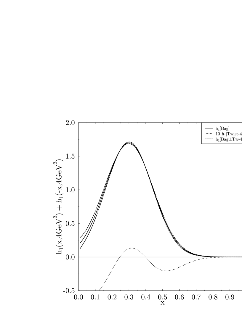
The IR-renormalon ambiguities shown in Fig. 1 are calculated using the bag model calculation of [6] for $h_{1}(x)$. The large $N_{f}$-limit is most reliable in the region of medium large Bjorken-$x$. For small $x$ the neglection of multiple gluon exchange is no longer justified. On the other hand the influence of the hadronic spectrum makes a pure perturbative calculation insufficient for large $x$. In the region of best accuracy ($0.2<x<0.45$) the uncertainty does not become bigger than 1% (see Fig. 2). One can expect a sizeable IR-renormalon uncertainty of up to 10% for $0.5<x<0.6$.

4 $\alpha_{s}$ corrections to the moments

It is possible to extract the anomalous dimension and the $\alpha_{s}$ corrections to the moments of the nonsinglet transversity distribution from Eq. (3). This expression has to be renormalized so that the Borel transformed Wilson coefficient should be regularized simultaneously analytically β€” like it was done in the previous section β€” and dimensionally. We get for this generalized expression ($d=4-\varepsilon$):

ℬ1as​[Cn​(Q2ΞΌ2,as)]​(s)=βˆ’CF​(ΞΌ2​eβˆ’CQ2)s​(4​π​μ2Q2)Ξ΅2​Γ​(2βˆ’Ξ΅2)​Γ​(βˆ’Ξ΅2βˆ’s)Γ​(3βˆ’Ξ΅βˆ’s)​Γ​(1+s)subscriptℬ1subscriptπ‘Žπ‘ delimited-[]subscript𝐢𝑛superscript𝑄2superscriptπœ‡2subscriptπ‘Žπ‘ π‘ subscript𝐢𝐹superscriptsuperscriptπœ‡2superscript𝑒𝐢superscript𝑄2𝑠superscript4πœ‹superscriptπœ‡2superscript𝑄2πœ€2Ξ“2πœ€2Ξ“πœ€2𝑠Γ3πœ€π‘ Ξ“1𝑠\displaystyle{\cal B}_{\frac{1}{a_{s}}}\left[C_{n}\left(\frac{Q^{2}}{\mu^{2}},a_{s}\right)\right](s)\;=\;-C_{F}\left(\frac{\mu^{2}e^{-C}}{Q^{2}}\right)^{s}\left(\frac{4\pi\mu^{2}}{Q^{2}}\right)^{\frac{\varepsilon}{2}}\frac{\Gamma\left(2-\frac{\varepsilon}{2}\right)\Gamma\left(-\frac{\varepsilon}{2}-s\right)}{\Gamma\left(3-\varepsilon-s\right)\Gamma(1+s)}
$\displaystyle\Bigg{\{}\sum_{k=0}^{n}\frac{\Gamma(1+s+k)\Gamma\left(s+k+\frac{\varepsilon}{2}\right)}{\Gamma(1+k)\Gamma(2+s+k)}\left[\left(s+\frac{\varepsilon}{2}\right)\left(6(1-s)+(4-\varepsilon)(1-\varepsilon)\right)+4k(2-s-\varepsilon)\right]$
$\displaystyle-(2-\varepsilon)\frac{\Gamma\left(1+s+n+\frac{\varepsilon}{2}\right)}{\Gamma(1+n)}+\varepsilon s(2-s-\varepsilon)\frac{\Gamma\left(1+s+n+\frac{\varepsilon}{2}\right)\Gamma(1+s+n)}{\Gamma(3+s+n)\Gamma(1+n)}\Bigg{\}}\quad.$ (25)

It is important to take care of a possible violation of the Ward identities due to the analytic continuation of $\gamma_{5}$ to $d$-dimensions [19].

The coefficients of the perturbative series can be reconstructed from the Borel transformed Wilson coefficient by an appropriate number of derivations with respect to $s$ at the origin $s=0$ of the Borel plane:

Bn(k+1)=Ξ²0k​(dd​s)k​ℬ1as​(Cn)​(s)|s=0.superscriptsubscriptπ΅π‘›π‘˜1evaluated-atsuperscriptsubscript𝛽0π‘˜superscriptπ‘‘π‘‘π‘ π‘˜subscriptℬ1subscriptπ‘Žπ‘ subscript𝐢𝑛𝑠𝑠0B_{n}^{(k+1)}\;=\;\left.\beta_{0}^{k}\left(\frac{d}{ds}\right)^{k}{\cal B}_{\frac{1}{a_{s}}}\left(C_{n}\right)(s)\right|_{s=0}\quad. (26)

This may be verified starting with Eq. (13) and using

ℬ1as​(ask+1)​(t)=tkk!.subscriptℬ1subscriptπ‘Žπ‘ superscriptsubscriptπ‘Žπ‘ π‘˜1𝑑superscriptπ‘‘π‘˜π‘˜{\cal B}_{\frac{1}{a_{s}}}\left(a_{s}^{k+1}\right)(t)\;=\;\frac{t^{k}}{k{\rm!}}\quad. (27)

So the first order $\alpha_{s}$ correction is determined by setting $s=0$ in Eq. (4). We find the quark-quark anomalous dimension of the nonsinglet operator as the coefficient of the divergence at $d=4$:

$$\gamma_{\perp,n}\;=\;\frac{C_{F}}{4\pi^{2}}\left(\frac{1}{1+n}+\sum_{k=1}^{n}\frac{1}{k}\right)\quad.$$ (28)

This anomalous dimension is identical with the coefficient of the $1/s$-term in Eq. (3) in the pure analytical regularization, as it should be. In momentum space we get the corresponding splitting function

$$P_{\perp}^{qq}(x)\;=\;\frac{C_{F}}{4\pi^{2}}\left(1-\frac{1}{(1-x)_{+}}\right)$$ (29)

which is to be compared with the splitting function for $h_{1}$ as found in the literature [4]:

$$P_{\perp}^{qq}(x)\;=\;\frac{C_{F}}{4\pi^{2}}\left(1-\frac{1}{(1-x)_{+}}-\frac{3}{4}\delta(x-1)\right)\quad.$$ (30)

Both expressions differ by $\frac{3}{4}\delta(x-1)$. This term is not really calculated in the conventional approach but rather fixed by the requirement that the transversity flip probability for quarks emitting a zero momentum gluon has to vanish.111We thank X. Artru for helpful comments. In addition the $\delta$-function part should be the same as for the polarized structure function $g_{1}$. Following this standard argumentation the corresponding $\delta(x-1)$-term has to be added in Eq. (29). However, such additional arguments should not be necessary in a direct calculation of the anomalous dimension. We got the right $\delta$-function in the case of $g_{1}$ without any additional arguments in an analogous calculation [15]. It is clear from a comparison of these two calculations that the behaviour of the anomalous dimensions of $g_{1}$ and $h_{1}$ at $x\to 1$ may only be indentical, if the vertex-correction with scalar- or vector-vertex contributes in the same way for $x\to 1$. This is obviously not the case, so that the difference of Eq. (29) and (30) at $x=1$ appears necessarily. Considering the general arguments leading to Eq. (30) as correct, we conclude that the equivalence of the twist-2 part of the used operator in Eq. (3) to $h_{1}$ leading to Eq. (29) is problematic at $x=1$. One should emphasize, however, that the renormalon estimation in the last section is not affected of this question.

Unlike in the case of $g_{1}$ [15] the anomalous dimension does not vanish for any $n$, so that at one loop level a renormalization is already necessary for all moments. We choose the $\overline{\rm MS}$-renormalization scheme. After renormalization of the Ward-identity with

Z5= 1βˆ’CF​αsΟ€+π’ͺ​(Ξ±s2)subscript𝑍51subscript𝐢𝐹subscriptπ›Όπ‘ πœ‹π’ͺsuperscriptsubscript𝛼𝑠2Z_{5}\;=\;1-C_{F}\,\frac{\alpha_{s}}{\pi}+{\cal O}(\alpha_{s}^{2}) (31)

we get for the first moments of the structure function defined by Eq. (3):

$\displaystyle\int_{0}^{1}dx\,\left(h_{1}(x)-\overline{h}_{1}(x)\right)\;=\;1+{\cal O}\left(\alpha_{s}^{2}\right)$
∫01𝑑x​x​(h1​(x)+hΒ―1​(x))= 1+78​CF​αsΟ€+π’ͺ​(Ξ±s2)superscriptsubscript01differential-dπ‘₯π‘₯subscriptβ„Ž1π‘₯subscriptΒ―β„Ž1π‘₯178subscript𝐢𝐹subscriptπ›Όπ‘ πœ‹π’ͺsuperscriptsubscript𝛼𝑠2\displaystyle\int_{0}^{1}dx\,x\left(h_{1}(x)+\overline{h}_{1}(x)\right)\;=\;1+\frac{7}{8}C_{F}\frac{\alpha_{s}}{\pi}+{\cal O}\left(\alpha_{s}^{2}\right)
∫01𝑑x​x2​(h1​(x)βˆ’hΒ―1​(x))= 1+138​CF​αsΟ€+π’ͺ​(Ξ±s2)superscriptsubscript01differential-dπ‘₯superscriptπ‘₯2subscriptβ„Ž1π‘₯subscriptΒ―β„Ž1π‘₯1138subscript𝐢𝐹subscriptπ›Όπ‘ πœ‹π’ͺsuperscriptsubscript𝛼𝑠2\displaystyle\int_{0}^{1}dx\,x^{2}\left(h_{1}(x)-\overline{h}_{1}(x)\right)\;=\;1+\frac{13}{8}C_{F}\frac{\alpha_{s}}{\pi}+{\cal O}\left(\alpha_{s}^{2}\right)
∫01𝑑x​x3​(h1​(x)+hΒ―1​(x))= 1+10948​CF​αsΟ€+π’ͺ​(Ξ±s2)superscriptsubscript01differential-dπ‘₯superscriptπ‘₯3subscriptβ„Ž1π‘₯subscriptΒ―β„Ž1π‘₯110948subscript𝐢𝐹subscriptπ›Όπ‘ πœ‹π’ͺsuperscriptsubscript𝛼𝑠2\displaystyle\int_{0}^{1}dx\,x^{3}\left(h_{1}(x)+\overline{h}_{1}(x)\right)\;=\;1+\frac{109}{48}C_{F}\frac{\alpha_{s}}{\pi}+{\cal O}\left(\alpha_{s}^{2}\right)
∫01𝑑x​x4​(h1​(x)βˆ’hΒ―1​(x))= 1+22780​CF​αsΟ€+π’ͺ​(Ξ±s2).superscriptsubscript01differential-dπ‘₯superscriptπ‘₯4subscriptβ„Ž1π‘₯subscriptΒ―β„Ž1π‘₯122780subscript𝐢𝐹subscriptπ›Όπ‘ πœ‹π’ͺsuperscriptsubscript𝛼𝑠2\displaystyle\int_{0}^{1}dx\,x^{4}\left(h_{1}(x)-\overline{h}_{1}(x)\right)\;=\;1+\frac{227}{80}C_{F}\frac{\alpha_{s}}{\pi}+{\cal O}\left(\alpha_{s}^{2}\right)\quad. (32)

As the used NNA-approximation is exact on the one-loop-level, these first order perturbative corrections are exact results.

5 Conclusions

We calculated the IR-renormalon ambiguity for the valence quark transversity distribution. The ambiguity is smaller than 1% in the region of best accuracy of the NNA-approximation. For $x\approx 0.6$ this systematic error becomes important reaching about 10%. Thus the renormalon uncertainty should be taken into accout when interpreting measurements of $h_{1}$ in this region of $x$. In addition we presented a calculation of the anomalous dimension using the operator in Eq. (3) and of the corresponding one loop perturbative corrections to the first moments. To our knowledge we calculated the perturbative corrections for the first time.

Acknowledgements. We thank L. Szymanowski and S. Hofmann for helpful discussions. This work has been supported by BMBF. A.S.Β thanks also the MPI fΓΌr Kernphysik in Heidelberg for support.

References

  • [1] J. Ralston, Davison E. Soper, Nucl. Phys. B152 (1979), 109.
    R.D. Tangerman, P.J. Mulders, Phys. Rev. D51 (1995), 3357-3372.
  • [2] G.R. Goldstein, Ann. Phys. 98 (1976), 128;
    Ann. Phys. 142 (1982), 219;
    Ann. Phys. 195 (1989), 213.
  • [3] R.L. Jaffe, The context of high energy QCD spin physics, in: Spin Structure of the nucleon. Wako, Japan 1995, S. 2-22.
  • [4] X. Artru, M. Mekhfi, Z.Phys. C45 (1990), 669-676.
  • [5] J. Soffer, Phys. Rev. Lett. 74 (1995), 1292.
    G.R. Goldstein, R.L. Jaffe, Xiangdong Ji, Phys. Rev. D52 (1995), 5006.
  • [6] R.L. Jaffe, Xiangdong Ji, Phys. Rev. Lett. 67 (1991), 552-555.
    Nucl. Phys. B375 (1992), 527.
  • [7] B.L. Ioffe, A. Khodjamirian, Phys. Rev. D51 (1995), 3373-3380.
  • [8] A.H. Mueller, Nucl. Phys. B250 (1985), 327-350.
    V.I. Zakharov, Nucl. Phys. B385 (1992), 452.
    A.H. Mueller, The QCD perturbation series, in: P.M. Zerwas, H.A. Kastrup (Hrsg.), QCD - 20 years later, Aachen 6/1992. World Scientific, Singapore, New Jersey, London, Hong Kong 1993, S. 162-171.
    P. Ball, M. Beneke, V.M. Braun, Nucl. Phys. B452 (1995), 563.
  • [9] A.H. Mueller, Phys. Lett. B308 (1993), 355.
    V.M. Braun, QCD renormalons and higher twist effects, in: Proceeding of 30th Rencontres de Moriond 1995: QCD and High Energy Hadronic Interaction, Meribel les Allues 1995.
  • [10] M. Beneke, V.M. Braun, Nucl. Phys. B454 (1995), 253.
  • [11] M. Beneke, Nucl. Phys. B405 (1993), 424-450.
    M. Beneke, V.M. Braun, Nucl. Phys. B426 (1994), 301-343.
  • [12] A.N. Vasilev, Yu.M. Pismak, J.R. Honkonen, Theor. Math. Phys. 46 (1981), 157.
    Theor. Math. Phys. 47 (1981), 291.
    J.A. Gracey, Mod. Phys. Lett. A7 (1992), 1945.
    Int. J. Mod. Phys. A8 (1993), 2465.
    Phys. Lett. B317 (1993), 415.
    Phys. Lett. B318 (1993), 177.
    AIHENP (1995), 259-264.
    Phys. Lett. B373 (1996), 178-184.
    M. Neubert, Phys. Rev. D51 (1995), 5924.
  • [13] D.J. Broadhurst, A.G. Grozin, Phys. Rev. D52 (1995), 4082.
    M. Beneke, V.M. Braun, Phys. Lett. B348 (1995), 513-520.
  • [14] E. Stein, M. Meyer-Hermann, L. Mankiewicz, A. SchΓ€fer, Phys. Lett. B376 (1996), 177-185.
  • [15] M. Meyer-Hermann, M. Maul, L. Mankiewicz, E. Stein, A. SchΓ€fer, Phys. Lett. B383 (1996), 463-469.
    Phys. Lett. B393 (E) (1997), 487.
  • [16] G. t’Hooft, Nucl. Phys. B72 (1974), 461.
    Edward Witten, Nucl. Phys. B160 (1979), 57.
  • [17] M. Dasgupta, B.R. Webber, Phys. Lett. B382 (1996), 273-281.
  • [18] Yu.L. Dokshitser, G. Marchesini, B.R. Webber, Nucl. Phys. B469 (1996), 93-142.
  • [19] S.A. Larin, J.A.M. Vermaseren, Phys.Lett. B259 (1991), 345-352.