On Effective Field Theories

at Finite Temperature

Jens O. Andersen

Thesis submitted for the Degree of

Doctor Scientiarum

Department of Physics

University of Oslo

June 1997

Abstract

This thesis is devoted to a study of quantum fields at finite temperature. First, I consider Dirac fermions and bosons moving in a plane with a homogeneous static magnetic field orthogonal to the plane. The effective action for the gauge field is derived by integrating out the matter field. The magnetization is calculated, and in the fermionic case it is demonstrated that the system exhibits de-Haas van Alphen oscillations at low temperatures and weak magnetic fields. I also briefly discuss the extension of the results to more general field configurations.

Next, the breakdown of ordinary perturbation theory at high temperature is studied. I discuss the need for an effective expansion and the resummation program of Braaten and Pisarski in some detail. The formalism is applied to Yukawa theory, and the screening mass squared and the free energy is derived to two and three loop order, respectively.

The main part of the present work is on effective field theories at finite temperature. I discuss the concepts of dimensional reduction, modern renormalization theory, and renormalizable field theories (“fundamental theories”) versus non-renormalizable theories (“effective theories”).

Two methods for constructing effective three dimensional field theories are discussed. The first is based on the effective potential, and is applied to field theory with $N$ charged $U(N)$ symmetric scalar coupled to an Abelian gauge field. The effective theory obtained may be used to study phase transition non-perturbatively as a function of $N$. The second method is an effective field theory approach based on diagrammatical methods, recently developed by Braaten and Nieto. I apply the method to spinor and scalar QED, and the screening masses as well the free energies are obtained.

Contents

1. Acknowledgments
2. Abstract
3. Preface
4. 1 Particles in External Fields
   1. 1.1 Introduction
   2. 1.2 Fermions in a Constant Magnetic Field
      1. 1.2.1 The Dirac Equation
      2. 1.2.2 The Fermion Propagator
      3. 1.2.3 The Effective Action
      4. 1.2.4 Magnetization and the de Haas-van Alphen Effect
      5. 1.2.5 Induced Vacuum Charges and Currents
      6. 1.2.6 Conductivity and the Integer Quantum Hall Effect
   3. 1.3 Bosons in a Constant Magnetic Field
      1. 1.3.1 The Klein-Gordon Equation
      2. 1.3.2 Boson Propagators and the Effective Action
      3. 1.3.3 Magnetization
   4. 1.4 Bosons in Constant Electromagnetic Fields
      1. 1.4.1 Pair Production in an Electric Field
   5. 1.5 Concluding Remarks
5. 2 Resummation and Effective Expansions
   1. 2.1 Introduction
   2. 2.2 The Breakdown of Perturbation Theory
   3. 2.3 A Simplified Resummation Scheme
   4. 2.4 The Screening Mass to Two-loop Order
   5. 2.5 Free Energy in Yukawa Theory to order $\lambda^{2}$, $\lambda g^{2}$ and $g^{4}$
6. 3 Effective Field Theory Approach I
   1. 3.1 Introduction
   2. 3.2 Finite Temperature
   3. 3.3 Spontaneously Broken Gauge Theories
   4. 3.4 The Two-loop Effective Potential
   5. 3.5 The Short-distance Coefficients
      1. 3.5.1 The Field Normalization Constants
      2. 3.5.2 The Coupling Constants
      3. 3.5.3 The Mass Parameters
   6. 3.6 The Middle-distance Coefficients
      1. 3.6.1 The Field Normalization Constants
      2. 3.6.2 The Coupling Constants
      3. 3.6.3 The Mass parameter
7. 4 Effective Field Theory Approach II
   1. 4.1 Introduction
   2. 4.2 QED at High Temperature
   3. 4.3 The Short-distance Coefficients
      1. 4.3.1 The Coupling Constant
      2. 4.3.2 The Mass Parameter
      3. 4.3.3 The Coefficient of the Unit Operator
   4. 4.4 The Free Energy and the Electric Screening Mass
   5. 4.5 QED Versus QCD
   6. 4.6 Electrostatic Scalar Electrodynamics
   7. 4.7 The Parameters in ESQED
      1. 4.7.1 The Coupling Constants
      2. 4.7.2 The Mass Parameters
      3. 4.7.3 The Coefficient of the Unit Operator
   8. 4.8 Calculations in ESQED
   9. 4.9 Summary and further Outlook
8. 5 Conclusions
9. A Sum-integrals in the Full Theory
10. B Integrals in the Effective Theory
11. C Some Sample Calculations
12. Bibliography

List of Figures

1. 1.1 The energy spectra of Dirac fermions in the presence of a constants magnetic field. a) $m>0$ and b) $m<0$.
2. 1.2 The density in units of $eB/2\pi$ as a function of $\mu/m$ for $T/m=1/1000$ (solid line) and for $T/m=1/100$ (dotted line). $eB/m^{2}=1$.
3. 1.3 The magnetization in units of $em$ as a function of $B$ in units of $m^{2}/e$ for different values of temperature. $\mu/m=3/2$.
4. 1.4 Magnification of the oscillatory region in Fig. 1.4.
5. 1.5 Thermal and vacuum contributions to the magnetization for a Fermi gas.
6. 1.6 The magnetization in units of $em$ as a function of $B$ in units of $m^{2}/e$ at $T=1/100$ and constant density $\rho/m^{2}=1$.
7. 1.7 The vacuum and thermal contributions to the magnetization for a Bose gas.
8. 2.1 One-loop correction to the two-point function in scalar theory.
9. 2.2 One-loop correction to the four-point function in scalar theory.
10. 2.3 The two-loop graphs for the two-point function.
11. 2.4 Ring diagrams in scalar theory.
12. 2.5 Diagrams contributing in the recalculation of the screening mass in scalar theory.
13. 2.6 One-loop fermion self-energy correction in Yukawa theory.
14. 2.7 Leading order contributions to the screening mass in Yukawa theory.
15. 2.8 Two-loop scalar diagrams.
16. 2.9 One-loop graph with a thermal counterterm insertion.
17. 2.10 Two-loop self-energy diagrams from the Yukawa sector.
18. 2.11 Mixed two-loop diagram contributing to the screening mass.
19. 2.12 One-loop graphs with wave function counterterm insertion in Yukawa theory.
20. 2.13 Infinite string of diagrams with scalar self-energy insertions.
21. 2.14 One-loop contributions to the free energy in Yukawa theory.
22. 2.15 Two-loop vacuum graphs.
23. 2.16 One-loop diagram with a thermal counterterm.
24. 2.17 Definition of the shaded blob.
25. 2.18 Infrared finite combination of diagrams.
26. 2.19 Infrared safe three-loop diagrams in Yukawa theory.
27. 2.20 Two-loop vacuum graphs with wave function counterterm insertions in Yukawa theory.
28. 3.1 Matching two-point functions at low energy.
29. 3.2 Light-by-light scattering in full QED, which can be mimicked by a local interaction on the scale $\Lambda\ll m$.
30. 3.3 One-loop correction to $\gamma$-$\gamma$ scattering in the Euler-Heisenberg Lagrangian.
31. 3.4 The tadpole graph, whose contributions from light and heavy modes have been separated.
32. 3.5 The one-loop diagrams in the effective theory appearing in the matching procedure.
33. 3.6 The two-loop graphs for the two-point function, where the contributions from the light and heavy particles have been separated explicitly.
34. 3.7 The two-loop graphs for the two-point function, in the three-dimensional theory.
35. 3.8 One-loop graphs contributing to the effective potential.
36. 3.9 Two-loop graphs contributing to the effective potential.
37. 3.10 One-loop counterterm diagrams for the effective potential.
38. 3.11 One-loop diagrams relevant for field strength normalization.
39. 3.12 One-loop diagrams needed for the calculating the couplings $e^{2}_{E}(\Lambda)$ and $h^{2}_{E}(\Lambda)$.
40. 3.13 One-loop four-point function with external timelike photon lines.
41. 3.14 Relevant graphs for integrating over the real scalar field $A_{0}$.
42. 4.1 One-loop, four point function with external timelike photon lines.
43. 4.2 One-loop self-energy graph in full QED.
44. 4.3 Two-loop self-energy graphs for $\Pi_{00}$ at zero external momentum.
45. 4.4 One-loop counterterm diagrams which cancel due to the Ward identity.
46. 4.5 One-loop self-energy correction in the effective theory.
47. 4.6 One-loop vacuum diagrams in QED.
48. 4.7 Two-loop vacuum diagrams in QED.
49. 4.8 Three-loop vacuum diagrams contributing to three free energy in QED.
50. 4.9 Two-loop counterterm diagrams in QED. The first two cancel since $Z_{1}=Z_{2}$.
51. 4.10 Loop diagrams in the effective theory.
52. 4.11 Example of a vanishing two-loop diagrams in magnetostatic QED.
53. 4.12 One-loop scalar self-energy diagrams in SQED.
54. 4.13 One-loop self-energy diagrams in the full theory.
55. 4.14 Two-loop self-energy diagrams in the full theory.
56. 4.15 One-loop vacuum diagrams in SQED.
57. 4.16 Two-loop diagrams for the free energy.
58. 4.17 Three-loop diagrams for the free energy.
59. 4.18 One and two-loop self-energy diagrams in the effective theory.
60. 4.19 One and two-loop diagrams contributing to the free energy in ESQED.

Preface

The thesis is based upon the following papers

• Magnetization in (2+1)-dimensional QED at Finite Temperature and density. Jens O. Andersen and Tor Haugset, Phys. Rev. D 51, 3073, 1995.

• Effective Potentials and Symmetry Restoration in the Chiral Abelian Higgs Model, Jens O. Andersen, Mod. Phys. Lett A 10 997, 1995.

• The Free Energy of High Temperature QED to Order $e^{5}$ From Effective Field Theory, Jens O. Andersen, Phys. Rev. D 53, 7286, 1996.

• The Electric Screening Mass in Scalar Electrodynamics at High Temperature, Jens O. Andersen, To appear in Z. Phys. C. 75, 1997.

• The Free Energy in Scalar Electrodynamics at High Temperature. Effective Field Theory versus Resummation, Jens O. Andersen, in preparation.

Chapter 1 Particles in External Fields

1.1 Introduction

One of the oldest problems in nonrelativistic quantum mechanics is that of a charged particle in a constant magnetic field. This problem was solved in 1930 by Landau [1], and the energy levels are called Landau levels.

More generally, particles in external fields have been studied extensively since the early fifties, when Schwinger [2] calculated the effective action for constant field strengths in QED using the proper time method. The study of matter under extreme conditions such as very strong electromagnetic fields is of interest in various systems, and the applications range from condensed matter to astrophysics [3,4].

In the case of a constant magnetic field there exists another and perhaps simpler method for obtaining the effective action of the gauge field [5]. Integrating out the fermion fields in the path integral gives rise to a functional determinant, that must be evaluated. In order to do so we exploit the fact that the propagator equals the derivative of the effective Lagrangian with respect to the mass in the fermionic case, and with respect to the squared of the mass in the bosonic case. This requires the knowledge of the propagator, which can be constructed explicitly, since we know the solutions to the Dirac equation or the Klein-Gordon equation in the case of a constant magnetic field.

Moreover, this method immediately generalizes to finite temperature and nonvanishing chemical potential. Thus, it becomes easy to study fermions and bosons at finite temperature and density.

So far the gauge field has been treated classically. However, one may of course consider quantum fluctuations around the classical background field. With the propagators at hand, one would then compute the vacuum diagrams in the loop expansion in the usual way. At the one loop level this implies a contribution to the effective action from the photons which equals $\frac{\pi^{2}T^{4}}{45}$. in 3+1$d$, and $\frac{\zeta(3)T^{3}}{\pi}$ in $2+1d$. This is the usual contribution to the free energy from a free photon gas at temperature $T$. Beyond one loop the evaluation of the graphs becomes difficult. Ritus has carried out one of the very few existing two-loop calculations in $3+1d$ QED at $T=0$, but finite density [6].

Many of the phenomena that have been discovered in condensed matter physics over the last few decades are to a very good approximation two dimensional. The most important of these are the (Fractional) Quantum Hall effect and high $T_{c}$ superconductivity [7].

Quantum field theories in lower dimensions have therefore become of increasing interest in recent years. Both systems mentioned above have been modeled by anyons, which are particles or excitations that obey fractional statistics. Anyons can be described in terms of Chern-Simons field theories [7-9].

Some ten years ago Redlich [10] considered fermions in a plane moving in a constant electromagnetic field. Using Schwinger’s proper time method [2] to obtain the effective action for the gauge field, he demonstrated that a Chern-Simons term is induced by radiative corrections. The Chern-Simons term is parity breaking and is gauge-invariant modulo surface terms.

External electromagnetic fields may give rise to induced charges in the Dirac vacuum if the energy spectrum is asymmetric with respect to some arbitrarily chosen zero point. The vacuum charge comes about since the number of particles gets reduced (or increased) relative to the free case. Furthermore, induced currents may appear and are attributed to the drift of the induced charges. This only happens if the external field does not respect the translational symmetry of the system. These interesting phenomena have been examined in detail by Flekkøy and Leinaas [11] in connection with magnetic vortices and their relevance to the Hall effect has been studied by Fumita and Shizuya [12].

In this chapter we re-examine the system considered by Redlich [10]. We shall restrict ourselves to the case of a constant magnetic field, but we extend the analysis by including thermal effects and we shall mainly focus on the magnetization of the system. For completeness, we also consider bosons in a constant magnetic field. Our calculations resemble the treatment given by Elmfors et al. [5] of the corresponding system in $3+1d$. However, interesting differences occur, mainly connected with the asymmetry in the Dirac spectrum, and we shall comment upon them as we proceed.

1.2 Fermions in a Constant Magnetic Field

We start our discussion of particles in external fields by considering fermions in two dimensions in a constant magnetic field.

1.2.1 The Dirac Equation

In this subsection we shall discuss some properties of the Dirac equation equation in $2+1d$. We also solve it for the case of a constant magnetic field along the $z$-axis. The Dirac equation reads

$$(i\gamma^{\mu}\partial_{\mu}-e\gamma^{\mu}A_{\mu}-m)\psi=0,$$ (1.1)

where the gamma matrices satisfy the Clifford algebra

$$\{\gamma^{\mu},\gamma^{\nu}\}=2g^{\mu\nu}.$$ (1.2)

In 2+1 dimensions the fundamental representation of the Clifford algebra is given by $2\times 2$ matrices and these can be constructed from the Pauli matrices. They are

$$\sigma^{1}=\left(\begin{array}[]{cc}0&1\\ 1&0\\ \end{array}\right),\hskip 28.45274pt\sigma^{2}=\left(\begin{array}[]{cc}0&-i\\ i&0\\ \end{array}\right),\hskip 28.45274pt\sigma^{3}=\left(\begin{array}[]{cc}1&0\\ 0&-1\\ \end{array}\right).$$ (1.3)

Furthermore, in $2+1d$ there are two inequivivalent choices of the gamma matrices, which corresponds to $\gamma^{\mu}\rightarrow-\gamma^{\mu}$. From Eq. (1.1) we see that this extra degree of freedom may be absorbed in the sign of $m$. These choices correspond to “spin up” and “spin down”, respectively [11].

The angular momentum operator $\sigma$ is a pseudo vector in $2+1d$, implying that the Dirac equation written in terms of these matrices does not respect parity [13]. This is no longer the case if the Dirac equation is expressed in terms of $4\times 4$ matrices. These matrices can be taken as the standard representation in $3+1d$

$$\gamma^{0}_{4}=\left(\begin{array}[]{cc}I&0\\ 0&I\\ \end{array}\right),\hskip 28.45274pt\gamma^{i}_{4}=\left(\begin{array}[]{cc}0&-\sigma^{i}\\ \sigma^{i}&0\\ \end{array}\right),$$ (1.4)

where we simply drop $\gamma^{3}_{4}$. This representation is reducible, and reduces to the two inequivalent fundamental representation mentioned above [13].

In the following we make the choice $\gamma^{0}=\sigma^{3}$, $\gamma^{1}=-i\sigma^{2}$ and $\gamma^{2}=-i\sigma^{1}$. In this chapter we use the real time formalism and the metric is $\mbox{diag}(1,-1,-1)$. For particles in a constant magnetic field, there are two convenient choices of the vector potential. These are $A_{\mu}=(0,By/2,-Bx/2)$ and $A_{\mu}=(0,0,-Bx)$, and are termed the symmetric and asymmetric gauge, respectively. In the first case the Hamiltonian commutes with the angular momentum operator and the solutions are given by Laguerre polynomials. In the second case we have $[H,p_{y}]=0$ and the solutions are Hermite polynomials (see below). We have chosen the asymmetric gauge and the Dirac equation then takes the form

$$\left(\begin{array}[]{cc}i\frac{\partial}{\partial t}-m&i\frac{\partial}{\partial x}-ieBx+\frac{\partial}{\partial y}\\ -i\frac{\partial}{\partial x}-ieBx+\frac{\partial}{\partial y}&-i\frac{\partial}{\partial t}-m\\ \end{array}\right)\psi({\bf x},t)=0.$$ (1.5)

Here $\psi({\bf x},t)$ is a two component spinor. Since the Hamiltonian commutes with $p_{y}$, we can write the wave functions as

$$\psi_{\kappa}({\bf x},t)=\exp(-iEt+iky)\left(\begin{array}[]{c}f_{\kappa}(x)\\ g_{\kappa}(x)\\ \end{array}\right),\hskip 28.45274pt$$ (1.6)

where ${\kappa}$ denotes all quantum numbers necessary in order to completely characterize the solutions. Inserting this into Eq. (1.5) one obtains

$$\left(\begin{array}[]{cc}E-m&-\xi_{+}\\ \xi_{-}&-E-m\\ \end{array}\right)=\left(\begin{array}[]{c}f_{\kappa}(x)\\ g_{\kappa}(x)\\ \end{array}\right),$$ (1.7)

where

$$\xi_{\pm}=-i\partial_{x}\mp i(k-eBx).$$ (1.8)

The equation for $f_{\kappa}(x)$ is readily found from Eq. (1.7):

$$\left(E^{2}-m^{2}-\xi_{+}\xi_{-}\right)f_{\kappa}(x)=0.$$ (1.9)

The eigenfunctions of $\xi_{+}\xi_{-}$, provided that $eB>0$, are [14]

$$I_{n,k}=(\frac{eB}{\pi})^{\frac{1}{4}}\exp\left[\,-\frac{1}{2}(x-\frac{k}{eB})^{2}eB\,\right]\frac{1}{\sqrt{n!}}H_{n}\left[\,\sqrt{2eB}(x-\frac{k}{eB})\,\right].$$ (1.10)

Here, $H_{n}(x)$ is the $n$th Hermite polynomial. Furthermore, $I_{n,k}(x)$ is normalized to unity and satisfies

$$\xi_{-}I_{n,k}(x) = -i\sqrt{2eBn}I_{n-1,k}(x),$$

$$\xi_{+}I_{n,k}(x) = i\sqrt{2eB(n+1)}I_{n+1,k}(x).$$

Combining eqs. (1.9) and (1.10) yields

$$f_{\kappa}(x)=I_{n,k}(x),\hskip 28.45274ptE^{2}=m^{2}+2eBn.$$ (1.11)

The function $g_{\kappa}(x)$ satisfies

$$g_{\kappa}(x)=\frac{\xi_{-}}{E+m}f_{\kappa}(x),$$ (1.12)

implying that

$$g_{\kappa}(x)=-i\sqrt{2eBn}I_{n-1,k}(x).$$ (1.13)

The normalized eigenfunctions become

$$\psi_{n,k}^{(\pm)}({\bf x},t)=\exp(\mp iE_{n}t+iky)\sqrt{\frac{E_{n}\pm m}{2E_{n}}}\left(\begin{array}[]{c}I_{n,k}(x)\\ \frac{\mp i\sqrt{2eBn}}{E_{n}\pm m}I_{n-1,k}(x)\\ \end{array}\right),$$ (1.14)

where $n=0,1,2,...$, $E_{n}=\sqrt{m^{2}+2eBn}$ and $\psi_{n,k}^{(\pm)}({\bf x},t)$ are positive and negative energy solutions, respectively. Note that $\psi^{(-)}_{0,k}({\bf x},t)=0$ and that we have defined $I_{-1,k}(x)\equiv 0$. The spectrum is therefore asymmetric and this asymmetry is intimately related to the induced vacuum charge, as will be shown in subsection LABEL:ladningi. In Fig. 1.1 a) we have shown the spectrum for $m>0$ and in Fig. 1.1 b) for $m<0$.

Figure 1.1: The energy spectra of Dirac fermions in the presence of a constants magnetic field. a) $m>0$ and b) $m<0$.

The field may now be expanded in the complete set of eigenmodes:

$$\Psi({\bf x},t)=\sum_{n=0}^{\infty}\int\frac{dk}{2\pi}\left[\,b_{n,k}\psi_{n,k}^{(+)}({\bf x},t)+d_{n,k}^{\,\ast}\psi_{n,k}^{(-)}({\bf x},t)\,\right].$$ (1.15)

Quantization is carried out in the usual way by promoting the Fourier coefficients to operators satisfying

$$\{b_{n,k},b_{n^{\prime},k^{\prime}}^{\dagger}\}=\delta_{n,n^{\prime}}\delta_{k,k^{\prime}},\hskip 28.45274pt\{d_{n,k},d_{n^{\prime},k^{\prime}}^{\dagger}\}=\delta_{n,n^{\prime}}\delta_{k,k^{\prime}},$$ (1.16)

and all other anti-commutators being zero.

1.2.2 The Fermion Propagator

In the previous section we solved the Dirac equation and with the wave functions at hand, we can construct the propagator. In vacuum it is defined by

$$iS_{F}(x^{\prime},x)=\langle 0\!\mid T\Big{[}\,\Psi({\bf x}^{\prime},t^{\prime})\overline{\Psi}({\bf x},t)\,\Big{]}\mid\!0\rangle,$$ (1.17)

where $T$ denotes time ordering. By use of the expansion (1.15) one finds

$$iS_{F}(x^{\prime},x)=\sum_{n=0}^{\infty}\int\frac{dk}{2\pi}\left[\,\theta(t^{\prime}-t)\psi^{(+)}_{n,k}({\bf x}^{\prime},t^{\prime})\overline{\psi}_{n,k}^{(+)}({\bf x},t)-\theta(t-t^{\prime})\psi^{(-)}_{n,k}({\bf x}^{\prime},t^{\prime})\overline{\psi}_{n,k}^{(-)}({\bf x},t)\,\right].$$ (1.18)

The step function has the following integral representation

$$\theta(t^{\prime}-t)=\frac{1}{2\pi i}\int\frac{e^{-\omega(t^{\prime}-t)}}{\omega-i\epsilon}d\omega.$$ (1.19)

After some purely algebraic manipulations, we obtain

$$S_{F}(x^{\prime},x)_{ab} = \frac{1}{4\pi^{2}}\sum_{n=0}^{\infty}\int dkd\omega\frac{E_{n}+m}{2E_{n}}\exp\left[\,-i\omega(t^{\prime}-t)+ik(y^{\prime}-y)\,\right]\times$$ (1.20)

$$\frac{1}{\omega^{2}-E^{2}_{n}+i\varepsilon}S_{ab}(n,\omega,k).$$

Here $S_{ab}(n,\omega,k)$ is the matrix

$$\left(\begin{array}[]{cc}(m+\omega)I_{n,k}(x^{\prime})I_{n,k}(x)&-i\sqrt{2eBn}I_{n,k}(x^{\prime})I_{n-1,k}(x)\\ -i\sqrt{2eBn}I_{n-1,k}(x^{\prime})I_{n,k}(x)&(m-\omega)I_{n-1,k}(x^{\prime})I_{n-1,k}(x)\\ \end{array}\right).$$ (1.21)

At finite temperature and chemical potential we write the thermal propagator as (see Ref. [5] for details)

$$\langle S_{F}(x^{\prime},x)\rangle_{\beta,\mu}=S_{F}(x^{\prime},x)+S_{F}^{\beta,\mu}(x^{\prime},x).$$ (1.22)

The thermal part of the propagator is

$$iS_{F}^{\beta,\mu}(x^{\prime},x)=-\sum_{n=0}^{\infty}\int\frac{dk}{2\pi}\left[\,f^{+}_{F}(E_{n})\psi^{(+)}_{n,k}({\bf x}^{\prime},t^{\prime})\overline{\psi}_{n,k}^{(+)}({\bf x},t)-f^{-}_{F}(E_{n})\psi^{(-)}_{n,k}({\bf x}^{\prime},t^{\prime})\overline{\psi}_{n,k}^{(-)}({\bf x},t)\,\right],$$ (1.23)

where

$$f^{(+)}_{F}(\omega)=\frac{1}{\exp\beta(\omega-\mu)+1},\hskip 28.45274ptf^{(-)}_{F}(\omega)=1-f^{(+)}_{F}(-\omega)=\frac{1}{\exp\beta(\omega+\mu)+1}.$$ (1.24)

This may be rewritten as

$$S_{F}^{\beta,\mu}(x^{\prime},x)=\frac{i}{2\pi}\sum_{n=0}^{\infty}\int dkd\omega\,\exp ik(y^{\prime}-y)\exp i\omega(t^{\prime}-t)f_{F}(\omega)\delta(\omega^{2}-E^{2}_{n}-i\varepsilon)S_{ab}(n,\omega,k).$$ (1.25)

Here

$$f_{F}(\omega)=\theta(\omega)F^{(+)}_{F}(\omega)+\theta(-\omega)F_{F}^{(-)}(\omega).$$ (1.26)

As noted in Ref. [5], one is not restricted to use equilibrium distributions in this approach. Single particle non-equilibrium distributions may be more appropriate if e.g. an electric field has driven the system out of equilibrium.

1.2.3 The Effective Action

The generating functional for fermionic Greens functions in an external magnetic field may be written as a path integral:

$$Z(\eta,\overline{\eta},A_{\mu})=\int{\cal D}\psi\,{\cal D}\overline{\psi}\exp\left[\,i\int d^{\,3}x\,\left(-\frac{1}{4}F_{\mu\nu}F^{\mu\nu}+\overline{\psi}(iD\!\!\!\!/-m)\psi-\overline{\eta}\psi+\overline{\psi}\eta\right)\,\right].$$ (1.27)

The functional integral describes the interaction of fermions with a classical electromagnetic field. It includes the effects of all virtual electron-positron pairs, but virtual photons are not present. Taking this into account at the one-loop simply amounts to including a temperature dependent, but field independent term in ${\cal L}_{\mbox{\scriptsize eff}}$.

The fermion field can be integrated over since the functional integral is Gaussian:

$$Z(\eta,\overline{\eta},A_{\mu})=\det[\,i(iD\!\!\!\!/-m)\,]\exp\Big{[}\,i\int d^{\,3}x\,\,\big{[}\,-\frac{1}{4}F_{\mu\nu}F^{\mu\nu}+\int d^{\,3}y\overline{\eta}(x)S_{F}(x,y)\eta(y)\,\big{]}\,\Big{]}.$$ (1.28)

Taking the logarithm of $Z(\eta,\overline{\eta},A_{\mu})$ with vanishing sources gives the effective action

$$S_{\mbox{\scriptsize eff}}=\int d^{\,3}x\left[\,-\frac{1}{4}F_{\mu\nu}F^{\mu\nu}\,\right]-i\,\mbox{Tr}\log\left[\,i(iD\!\!\!\!/-m)\,\right].$$ (1.29)

Note that we have written $\log\det=\mbox{Tr}\,\log$ by the use of a complete orthogonal basis and that the trace is over space-time as well as spinor indices. Differentiating Eq. (1.29) with respect to $m$ yields

$$\frac{\partial{\cal L}_{1}}{\partial m}=i\,\mbox{tr}S_{F}(x,x).$$ (1.30)

The trace is now over spinor indices only. By calculating the trace of the propagator and integrating this expression with respect to $m$ thus yields the one-loop contribution to the effective action. This method has been previously applied by Elmfors et al. [5] in 3+1 dimensions.

The above equation may readily be generalized to finite temperature, where we separate the vacuum contribution in the effective action

$${\cal L}={\cal L}_{0}+{\cal L}_{1}+{\cal L}^{\beta,\mu}\equiv{\cal L}_{0}+{\cal L}_{\mbox{\scriptsize eff}}$$ (1.31)

where ${\cal L}_{0}$ is the tree level contribution, and

$$\frac{\partial{\cal L}_{\mbox{\scriptsize eff}}}{\partial m}=i\,\mbox{tr}\left[\,S_{F}(x,x)+S_{F}^{\beta,\mu}(x,x)\,\right].$$ (1.32)

Using eqs. (1.20) and (1.21) a straightforward calculation gives for the vacuum contribution

$$\mbox{tr}S_{F}(x,x) = \frac{1}{4\pi^{2}}\sum_{n=0}^{\infty}\int\frac{dk\,d\omega}{\omega^{2}-E^{2}_{n}+i\varepsilon}\left[\,m\left(I_{n,k}^{2}(x)+I_{n-1,k}^{2}(x)\right)+\omega\left(I_{n,k}^{2}(x)-I_{n-1,k}^{2}(x)\right)\,\right]$$ (1.33)

$$= -\frac{i}{2\pi}\sum_{n=1}^{\infty}\int dk\frac{m}{E_{n}}I_{n,k}^{2}(x)-\frac{ieB}{4\pi}$$

$$= -\frac{ieB}{2\pi}\sum_{n=1}^{\infty}\frac{m}{E_{n}}-\frac{ieB}{4\pi}.$$

Integrating this expression with respect to $m$ yields

$${\cal L}_{1}=\frac{eB}{2\pi}\sum_{n=1}^{\infty}\sqrt{m^{2}+2eBn}+\frac{eBm}{4\pi}.$$ (1.34)

The divergence may be sidestepped by using the integral representation of the gamma function [15] and subtract a constant to make ${\cal L}_{1}$ vanish for $B=0$,

$${\cal L}_{1}=-\frac{1}{8\pi^{\frac{3}{2}}}\int_{0}^{\infty}\frac{ds}{s^{\frac{5}{2}}}\exp(-m^{2}s)\left[\,eBs\coth(eBs)-1\,\right].$$ (1.35)

This result calls for a few comments. We have chosen a gauge, where $A_{0}=0$. However, we could equally well have chosen $A_{0}$ to be a nonzero constant. This would give rise to an additional term in the effective action

$$\delta{\cal L}_{1}=-\frac{m}{|m|}\frac{e^{2}}{4\pi}A_{0}B.$$ (1.36)

This is simply the gauge dependent Chern-Simons term, whose existence first was demonstrated by Redlich [10].

In the following, we shall only consider $m>0$, except for subsection LABEL:ladningi. Similar results for $m<0$ can, of course, be obtained by the same methods.

The finite temperature part of the effective action is calculated analogously using the thermal part of the propagator (1.23).

$${\cal L}^{\beta,\mu} = \frac{TeB}{2\pi}\sum_{n=1}^{\infty}\Big{[}\,\log[\,1+\exp-\beta(E_{n}-\mu)\,]+\log[\,1+\exp-\beta(E_{n}+\mu)\,]\,\Big{]}$$ (1.37)

$$+\frac{TeB}{2\pi}\log\left[\,1+\exp-\beta(m-\mu)\,\right].$$

Letting $B\rightarrow 0$ it can be shown that one obtains the pressure of a gas of noninteracting electrons and positrons:

$${\cal L}_{0}^{\beta,\mu} = \frac{T}{2\pi}\int_{m}^{\infty}EdE\Big{[}\,\log[\,1+\exp-\beta(E-\mu)\,]+\log[\,1+\exp-\beta(E+\mu)\,]\,\Big{]}$$

$$= -\frac{mT^{2}}{2\pi}\Big{[}\mbox{Li}_{2}(-\lambda e^{-\beta m})+\mbox{Li}_{2}(-\lambda^{-1}e^{-\beta m})\Big{]}-\frac{T^{3}}{2\pi}\Big{[}\mbox{Li}_{3}(-\lambda e^{-\beta m})+\mbox{Li}_{3}(-\lambda^{-1}e^{-\beta m})\Big{]}.$$

Here, $\lambda=e^{\beta\mu}$ is the fugacity and $\mbox{Li}_{n}(x)$ is the polylogarithmic function of order $n$:

$$\mbox{Li}_{n}(x)=\sum_{k=1}^{\infty}\frac{x^{k}}{k^{n}}.$$ (1.39)

In the following we restrict ourselves to the case $\mu>0$. Analogous results can be obtained for $\mu<0$.

In the zero temperature limit of ${\cal L}^{\beta,\mu}$ one gets

$${\cal L}^{\beta,\mu}=\frac{eB}{2\pi}\sum_{n=0}^{\,\prime}(\mu-E_{n}),$$ (1.40)

where the prime indicates that the sum is restricted to integers less than $(\mu^{2}-m^{2})/2eB$.

Similarly, one may derive the density

$$\rho=\frac{\partial{\cal L}^{\beta,\mu}}{\partial\mu} = \frac{eB}{2\pi}\sum_{n=1}^{\infty}\Big{[}\frac{1}{\exp\beta(E_{n}-\mu)\,+1}-\frac{1}{\exp\beta(E_{n}+\mu)\,+1}\Big{]}$$

$$+ \frac{eB}{2\pi}\frac{1}{\exp\beta(m-\mu)\,+1}.$$

At $T=0$ this reduces to

$$\rho=\frac{eB}{2\pi}\Big{[}\mbox{Int}\,(\frac{\mu^{2}-m^{2}}{2eB})+1\Big{]},\hskip 28.45274pt\mu>m,$$ (1.42)

in accordance with the result of Zeitlin [16]. ¿From Eq. (1.42) one immediately finds that the density as a function of chemical potential for fixed magnetic field is a step function. This is intimately related to the integer Hall effect as noted in Ref. [17]. In Fig. 1.2 we have plotted the density as a function of chemical potential for low temperatures (dashes line: $T/m=1/100$, solid line: $T/m=1/1000$). One observes that the sharp edges get smeared out as the temperature increases.

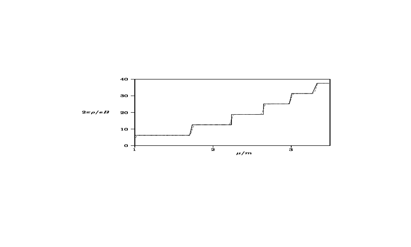
Figure 1.2: The density in units of $eB/2\pi$ as a function of $\mu/m$ for $T/m=1/1000$ (solid line) and for $T/m=1/100$ (dotted line). $eB/m^{2}=1$.

1.2.4 Magnetization and the de Haas-van Alphen Effect

In this section we study the physical content of the effective action which was obtained in the previous section. In particular we investigate a few limits to check the consistency of our calculations.

The magnetization is defined by [5]

$$M=\frac{\partial{\cal L}_{\mbox{\scriptsize eff}}}{\partial B}.$$ (1.43)

The vacuum contribution to the magnetization is obtained from Eq. (1.35)

$$M_{1}=-\frac{1}{8\pi^{\frac{3}{2}}}\int_{0}^{\infty}ds\frac{\exp\,(-m^{2}s)}{s^{\frac{5}{2}}}\left[\,es\coth(eBs)-\frac{e^{2}Bs^{2}}{\sinh^{2}(eBs)}\,\right].$$ (1.44)

For the thermal part of the magnetization we find

$$M^{\beta,\mu} = \frac{Te}{2\pi}\sum_{n=1}^{\infty}\Big{[}\,\log[\,1+\exp-\beta(E_{n}-\mu)\,]+\log[\,1+\exp-\beta(E_{n}+\mu)\,]\,\Big{]}$$ (1.45)

$$+\frac{Te}{2\pi}\log\big{[}\,1+\exp-\beta(m-\mu)\,\big{]}$$

$$-\frac{e^{2}B}{2\pi}\sum_{n=1}^{\infty}\frac{n}{E_{n}}\Big{[}\,\frac{1}{\exp\beta(E_{n}-\mu)+1}+\frac{1}{\exp\beta(E_{n}+\mu)+1}\,\Big{]}.$$

Magnetization at zero temperature.   In the zero temperature limit Eq. (1.45) reduces to

$$M^{\beta,\mu}=\frac{e}{2\pi}\sum^{\prime}_{n=0}\left[\,\mu-E_{n}-\frac{eBn}{E_{n}}\,\right],$$ (1.46)

where the sum again is restricted to integers less than $(\mu^{2}-m^{2})/2eB$. The thermal part of the magnetization at zero temperature changes abruptly, when $(\mu^{2}-m^{2})/2eB$ increases by unity. Thus, $M^{\beta,\mu}$ oscillates wildly, in particular is the limit $B\rightarrow 0$ not well defined. The strong field limit ($B\rightarrow\infty$) of $M^{\beta,\mu}$ is found to be

$$\frac{e}{2\pi}(\mu-m).$$ (1.47)

In the weak $B$-field limit ($eB\ll\mu^{2}-m^{2}\ll m^{2}$) the vacuum contribution becomes

$$M_{1}=-\frac{e^{2}B}{12\pi^{3/2}}\int_{0}^{\infty}ds\frac{\exp(-m^{2}s)}{s^{\frac{1}{2}}}=-\frac{e^{2}B}{12\pi|m|}.$$ (1.48)

This agrees with the results of Ref. [18]. In order to get the strong field limit $(\,eB\gg m^{2})$ of the vacuum contribution, we scale out $eB$ and take $eB\rightarrow\infty$ in the remainder. This gives

$${\cal L}_{1}\propto(eB)^{\frac{3}{2}}\Rightarrow M_{1}\propto e^{\frac{3}{2}}\sqrt{B}.$$ (1.49)

Vacuum effects contribute to the magnetization proportional to the square root of $B$. This should be compared with the corresponding result in $3+1d$, where the magnetization goes like $B\log(\frac{B}{m^{2}})$ [5]. The thermal part of the magnetization was found to be $M^{\beta,\mu}=e(\mu-m)/2\pi$. Hence, the vacuum contribution dominates, exactly as in $3+1d$. For $\mu\neq m$ we see that the thermal part of the magnetization is nonzero. From Eq. (1.42) one obtains $\rho=eB/2\pi$, so the nonzero magnetization is a consequence of the fact that the density increases as the magnetic field increases (since all particles are in the ground state).

Magnetization at finite temperature.   In Fig. 1.3 we have displayed the total magnetization as a function of the external magnetic field for different values of the temperature ($\mu/m=3/2$,  $T/m$ =1/150 solid line,  1/50 dashed line,  1/5 dotted line). Fig. 1.4 is a magnification of Fig. 1.3 in the oscillatory region.

The fermion gas exhibits the de Haas-van Alphen oscillations for small values of the magnetic field. These oscillations have been observed in many condensed matter systems [3], and they were first observed experimentally in 1930 [19]. It is a direct consequence of the Pauli exclusion principle and the discreteness of the spectrum.

We also note that the magnetization approaches a nonzero value as $B\rightarrow 0$. More specifically, in Ref. [20] it is demonstrated that the limit equals

$$M^{\beta,\mu}=\frac{Te}{2\pi}\ln\Bigg{[}\left(1+e^{-\beta(m-\mu)}\right)-\left(1+e^{-\beta(m+\mu)}\right)\Bigg{]}.$$ (1.50)

Some comments are in order. It is perhaps somewhat surprising that the magnetization is nonzero in this limit. One should, however, bear in mind that the sign of $m$ uniquely determines the spin of the particles (and antiparticles), implying that the system under investigation consists entirely of either spin up or spin down particles. This is not the case in $3+1d$, where the representations characterized by the sign of $m$ are equivalent. By summing over $\pm m$, or equivalently, by using four component spinors, one finds a vanishing magnetization as $B$ goes to zero, exactly as in $3+1$ dimensions.

Finally, we have displayed the modulus of the vacuum part as well as the thermal part of the magnetization over a rather broad interval of values of $eB/m^{2}$ in Fig. 1.5. ($T/m=1/5$ and $\mu/m=1.1$). The thermal contribution saturates for values of the field where the vacuum contribution starts to dominate. The reason is that all particles are in the lowest Landau level for high values of $B$, and that the energy of this level is independent of the magnetic field.

High Temperature Limit $(\,T^{2}\gg m^{2}\gg eB,\mu=0)$.   The high temperature limit is rather trivial. From a physical point of view, one expects that ${\cal L}^{\beta,\mu}$ approaches the thermodynamic potential of a gas of noninteracting particles of mass $m$. Indeed, in this limit, one may recover Eq. (1.2.3) by treating $n$ as a continuous variable.

Figure 1.3: The magnetization in units of $em$ as a function of $B$ in units of $m^{2}/e$ for different values of temperature. $\mu/m=3/2$.

Figure 1.4: Magnification of the oscillatory region in Fig. 1.4.

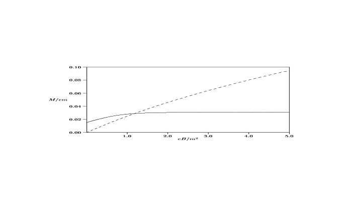
Figure 1.5: Thermal and vacuum contributions to the magnetization for a Fermi gas.

We would also like to describe the system in terms of constant charge density. At zero temperature it is not possible to invert Eq. (1.42) to write the chemical potential as a function of density, since the step function is not one-to-one. However, $\mu$ can be interpreted as the Fermi energy at $T=0$ (as long as the highest occupied Landau level is not completely filled), so one can immediately write down the chemical potential as a function of density:

$$\mu=\sqrt{m^{2}+2eB\,\mbox{Int}\,(\frac{2\pi\rho}{eB})}\,\,.$$ (1.51)

We should also point out that at $T>0$ there is a one-to-one correspondence between density and chemical potential (Fig. 1.2), so one can invert Eq. (1.2.3) numerically.

We have used Eq. (1.51) to make a plot of the thermal part of the magnetization as a function of magnetic field at constant density and at $T=1/100$. The resulting curve is displayed in Fig. 1.6.

Figure 1.6: The magnetization in units of $em$ as a function of $B$ in units of $m^{2}/e$ at $T=1/100$ and constant density $\rho/m^{2}=1$.

The de Haas-van Alphen oscillations are seen to be present for low temperatures and weak magnetic fields. Furthermore, it is seen that the magnetization is zero for large magnetic fields. This can be understood from the following physical argument: For large $B$-fields all particles are in the lowest Landau level and $\mu=m$ (recall that the degeneracy increases linearly with $B$). The energy of the single particle ground state is independent of the external field ($E_{0}=m$), so increasing $B$ cannot lead to an increase in ${\cal L}^{\beta,\mu}$, when the charge density (and therefore the particle density) is held constant. Hence, the contribution to the magnetization from real thermal particles vanishes in the strong field limit.

1.2.5 Induced Vacuum Charges and Currents

In this subsection we calculate the vacuum expectation value of the induced charge and current densities. Such calculations have been carried out in other contexts, e.g. in connection with magnetic flux strings (see Ref. [11]). We shall employ the most commonly used definition of the current operator which can be shown to measure the spectral asymmetry relative to the spectrum of free Dirac particles.

$$j^{\mu}\,(x)=\frac{e}{2}\left[\,\overline{\Psi}_{\alpha}(x),\left(\gamma^{\mu}\Psi(x)_{\alpha}\right)\,\right].$$ (1.52)

Using the complete set of eigenmodes as given by Eq. (1.14), a straightforward calculation yields

$$\langle\,\rho\,(x)\,\rangle=-\frac{m}{\mid\!m\!\mid}\frac{e^{2}B}{4\pi}.$$ (1.53)

Eq. (1.53) is simply the Chern-Simons relation. It has previously been obtained by e.g. Zeitlin [16] using the proper time method. This result has the following physical interpretation: As we turn the magnetic field on, an unpaired energy level $E=m$ emerges (in the case $m>0$). The number of positrons therefore gets reduced relative to the free case. This can be interpreted as the appearance of electrons and results in a negative charge density. For $m<0$ a similar argument applies.

A corresponding calculation of $\langle\,{\bf j}\,(x)\,\rangle$ reveals that the induced current vanishes. This result should come as no surprise due to translational symmetry of the system. A nonvanishing vacuum current would arise in the presence of an external electric field and is then attributed to the drift of the induced vacuum charge.

1.2.6 Conductivity and the Integer Quantum Hall Effect

Let us next consider the conductivity. According to Ref. [21] the expression for the components of the conductivity $\sigma_{ij}$ can be expressed in terms of the polarization tensor $\Pi_{\mu\nu}(k_{0},{\bf k})$:

$$\sigma_{ij} = \left.i\frac{\partial\Pi_{0i}(0,{\bf k})}{\partial k_{j}}\right|_{{\bf k}\rightarrow 0},$$ (1.54)

and follows from linear response theory. Moreover, by considering the functional derivative of the effective action with respect to $A_{\mu}$ one may deduce that [21]

$$\Pi_{0i}(k_{0},{\bf k}\rightarrow 0)=-ie\epsilon_{ij}k_{j}\frac{\partial\rho}{\partial B}.$$ (1.55)

Combining the above equations, one may infer that

$$\sigma_{ij}=\sigma\epsilon_{ij}=\epsilon_{ij}e\frac{\partial\rho}{\partial B}.$$ (1.56)

Thus, the conductivity is Hall like. Using Eq. (1.2.3) and including the contribution from the induced vacuum charge, which was calculated in the previous section, we obtain

$$\sigma = -\frac{e^{2}}{4\pi}+\frac{e^{2}}{2\pi}\sum_{n=1}^{\infty}\Big{[}\frac{1}{1+\exp\beta(E_{n}-\mu)\,}-\frac{1}{1+\exp\beta(E_{n}+\mu)\,}\Big{]}+\frac{e^{2}}{2\pi}\frac{1}{1+\exp\beta(m-\mu)\,}$$ (1.57)

$$+\frac{e^{3}B}{2\pi T}\sum_{n=1}^{\infty}\frac{n}{E_{n}}\Big{[}\frac{\exp\beta(E_{n}-\mu)\,}{[1+\exp\beta(E_{n}-\mu)\,]^{2}}-\frac{\exp\beta(E_{n}+\mu)\,}{[1+\exp\beta(E_{n}+\mu)\,]^{2}}\Big{]}.$$

Letting $T\rightarrow 0$ one finds

$$\sigma=-\frac{e^{2}}{4\pi}+\frac{e^{2}}{2\pi}\mbox{Int}\left[\frac{\mu^{2}-m^{2}}{2eB}\right].$$ (1.58)

We thus see that the conductivity is a step function for $T=0$. The system therefore contains the integer Quantum Hall effect. This was also noted by Zeitlin [16]. The generalization of Zeitlin’s result to finite temperature is new.

1.3 Bosons in a Constant Magnetic Field

In this section we focus the attention on bosons in a constant magnetic field. We calculate the effective action and derive the magnetization. We point out the differences between the bosonic and fermionic results. Finally, we generalize to constant field strengths and study pair production in a purely electric field.

1.3.1 The Klein-Gordon Equation

Let us for the convenience of the reader briefly discuss the solutions to the Klein-Gordon equation in an external constant magnetic field. It reads

$$[D_{\mu}D^{\mu}+m^{2}]\phi({\bf x},t)=0,$$ (1.59)

where $D_{\mu}=\partial_{\mu}+ieA_{\mu}$ is the covariant derivative and the metric is diag ($1$, $-1$, $-1$). We have again chosen the asymmetric gauge $A_{\mu}=(0,0,-Bx)$ and assume that the wave functions are in the form

$$\phi({\bf x},t)=e^{-iEt+iky}f(x).$$ (1.60)

The differential equation for $f(x)$ then becomes

$$\xi_{-}\xi_{+}f(x)=(E^{2}-m^{2}+eB)f(x),$$ (1.61)

where $\xi_{\pm}$ were defined in Eq. (1.8) and the eigenfunctions of $\xi_{-}\xi_{+}$ were defined in Eq. (1.10). The normalized eigenfunctions of the Klein-Gordon equation are

$$\phi_{n,k}({\bf x},t)=e^{-iEt+iky}(\frac{eB}{\pi})^{\frac{1}{4}}\exp\left[-\frac{1}{2}(x-\frac{k}{eB})^{2}eB\right]\frac{1}{\sqrt{n!}}H_{n}\left[\sqrt{2eB}(x-\frac{k}{eB})\right],$$ (1.62)

with corresponding eigenvalues $E_{n}=\sqrt{m^{2}+(2n+1)eB}$. The Klein-Gordon field can now expanded in the complete set of solutions:

$$\Phi({\bf x},t)=\frac{1}{4\pi}\sum_{n=0}^{\infty}\int\frac{dk}{E_{n}}\Big{[}a_{n,k}\phi_{n,k}({\bf x},t)+b_{n,k}^{\ast}\phi_{n,k}^{\ast}({\bf x},t)\Big{]}.$$ (1.63)

Quantization is carried out as in the fermionic case by promoting the Fourier coefficients to operators. The only nonvanishing commutators are

$$[a_{n,k},a_{n^{\prime},k^{\prime}}^{\dagger}]=4\pi E_{n}\delta_{n,n^{\prime}}\delta(k-k^{\prime}),\hskip 28.45274pt[b_{n,k},b_{n^{\prime},k^{\prime}}^{\dagger}]=4\pi E_{n}\delta_{n,n^{\prime}}\delta(k-k^{\prime}).$$ (1.64)

1.3.2 Boson Propagators and the Effective Action

The generating functional for bosonic Greens functions in an external magnetic field may be written as a path integral in analogy with the fermionic case

$$Z(J,J^{\dagger},A_{\mu})=\int{\cal D}\phi\,{\cal D}\phi^{\dagger}\exp\left[i\int d^{\,3}x\left(-\frac{1}{4}F_{\mu\nu}F^{\mu\nu}+\phi^{\dagger}(D_{\mu}D^{\mu}+m^{2})\phi+J^{\dagger}\phi+\phi^{\dagger}J\right)\right].$$ (1.65)

We integrate out the bosons in the functional integral and get a functional determinant:

$$Z(J,J^{\dagger},A_{\mu})=\det[i(D_{\mu}D^{\mu}+m^{2})]\exp\Big{[}i\int d^{\,3}x\,\,\big{[}-\frac{1}{4}F_{\mu\nu}F^{\mu\nu}+\int d^{\,3}yJ^{\dagger}(x)\Delta_{F}(x,y)J(y)\big{]}\Big{]}.$$ (1.66)

Taking the logarithm of $Z(J,J^{\dagger},A_{\mu})$ with vanishing external sources gives the effective action

$$S_{\mbox{\scriptsize eff}}=\int d^{\,3}x\left[-\frac{1}{4}F_{\mu\nu}F^{\mu\nu}\right]-i\,\mbox{tr}\log\left[i(D_{\mu}D^{\mu}+m^{2})\right],$$ (1.67)

where we have written $\log\det=\mbox{Tr}\,\log$ by the use of a complete orthogonal basis. The first term is denoted ${\cal L}_{0}$ and is the tree level contribution. For a constant magnetic field we have ${\cal L}_{0}=-\frac{B^{2}}{2}$. Differentiating Eq. (1.67) with respect to $m^{2}$ yields

$$\frac{\partial{\cal L}_{1}}{\partial m^{2}}=-i\,\mbox{tr}\Delta_{F}(x,x).$$ (1.68)

The next step is then to construct the boson propagator which in vacuum is defined as

$$i\Delta_{F}(x^{\prime},x)=\langle 0\!\mid T\Big{[}\Phi({\bf x}^{\prime},t^{\prime})\Phi^{\dagger}({\bf x},t)\Big{]}\mid\!0\rangle.$$ (1.69)

Here, $T$ denotes time ordering as usual. By use of the expansion (1.63) one finds

$$\Delta_{F}(x^{\prime},x)=-\frac{i}{4\pi^{2}}\sum_{n=0}^{\infty}\int\frac{dk}{E_{n}}\left[\theta(t^{\prime}-t)\phi_{n,k}({\bf x}^{\prime},t^{\prime})\phi_{n,k}^{\ast}({\bf x},t)+\theta(t-t^{\prime})\phi_{n,k}({\bf x}^{\prime},t^{\prime})\phi_{n,k}^{\ast}({\bf x},t)\right].$$ (1.70)

After some algebraic manipulations and using the integral representation of the step function, we obtain

$$\Delta_{F}(x^{\prime},x) = \frac{1}{4\pi^{2}}\sum_{n=0}^{\infty}\int\frac{dkd\omega}{\omega^{2}-E^{2}_{n}+i\varepsilon}\exp\left[-i\omega(t^{\prime}-t)+ik(y^{\prime}-y)\right]I_{n}(x)I_{n}(x^{\prime}).$$ (1.71)

The trace then becomes

$$\mbox{tr}\Delta_{F}(x,x) = \frac{1}{4\pi^{2}}\sum_{n=0}\int\frac{dkd\omega}{\omega^{2}-E^{2}_{n}+i\varepsilon}I_{n}^{2}(x)$$

$$= -\frac{ieB}{4\pi}\sum_{n=0}^{\infty}\frac{1}{E_{n}}.$$

Integration with respect to $m^{2}$ gives the effective action:

$${\cal L}_{1}=-\frac{Be}{2\pi}\sum_{n=0}^{\infty}\sqrt{m^{2}+(2n+1)eB}\,.$$ (1.73)

Employing the integral representation of the $\Gamma$-function [15], we find

$${\cal L}_{1}=\frac{eB}{8\pi^{\frac{3}{2}}}\int_{0}^{\infty}\frac{ds}{s^{\frac{3}{2}}}e^{-m^{2}s}\Big{[}\frac{1}{\sinh(eBs)}-\frac{1}{eBs}\Big{]}.$$ (1.74)

The above expression has been rendered finite by requiring that ${\cal L}_{1}=0$ for $B=0$. This result is in accordance with the leading term in the derivative expansion employed by Cangemi et al. [18].

At finite temperature and chemical potential we write the thermal propagator as

$$\langle\Delta_{F}(x^{\prime},x)\rangle_{\beta,\mu}=\Delta_{F}(x^{\prime},x)+\Delta_{F}^{\beta,\mu}(x^{\prime},x).$$ (1.75)

The thermal part of the propagator is

$$i\Delta_{F}^{\beta,\mu}(x^{\prime},x)=-\frac{1}{4\pi}\sum_{n=0}^{\infty}\int\frac{dk}{E_{n}}\left[f^{+}_{B}(E_{n})\phi_{n,k}(x^{\prime})\phi^{\ast}_{n,k}(x)-f^{-}_{B}(E_{n})\phi_{n,k}(x^{\prime})\phi^{\ast}_{n,k}(x)\right].$$ (1.76)

Here $f^{(+)}_{B}(\omega)$ and $f^{(-)}_{B}(\omega)$ are the bosonic equilibrium distributions:

$$f^{(+)}_{B}(\omega)=\frac{1}{\exp\beta(\omega-\mu)-1},\hskip 28.45274ptf^{(-)}_{B}(\omega)=\frac{1}{\exp\beta(\omega+\mu)-1}.$$ (1.77)

Eq. (1.68) is easily generalized to finite temperature. Writing ${\cal L}={\cal L}_{0}+{\cal L}_{1}+{\cal L}^{\beta,\mu}\equiv{\cal L}_{0}+{\cal L}_{\mbox{\scriptsize eff}}$, we have

$$\frac{\partial{\cal L}_{\mbox{\scriptsize eff}}}{\partial m^{2}}=-i\,\mbox{tr}\Big{[}\Delta_{F}(x^{\prime},x)+\Delta_{F}^{\beta,\mu}(x^{\prime},x)\Big{]}.$$ (1.78)

Straightforward calculations give the thermal part of the effective action

$${\cal L}^{\beta,\mu}=-\frac{TeB}{2\pi}\sum_{n=1}^{\infty}\Big{[}\,\log[\,1-\exp-\beta(E_{n}-\mu)\,]+\log[\,1-\exp-\beta(E_{n}+\mu)\,]\,\Big{]}.$$ (1.79)

The limit $B\rightarrow 0$ is easily taken, and we find

$$\!\!\!\!\!\!{\cal L}^{\beta,\mu} = -\frac{T}{2\pi}\int_{m}^{\infty}DEE\Big{[}\,\log[\,1-\exp-\beta(E-\mu)\,]+\log[\,1-\exp-\beta(E+\mu)\,]\,\Big{]}$$ (1.80)

$$= \frac{mT^{2}}{2\pi}\Big{[}\mbox{Li}_{2}(\lambda e^{-\beta m})+\mbox{Li}_{2}(\lambda^{-1}e^{-\beta m})\Big{]}+\frac{T^{3}}{2\pi}\Big{[}\mbox{Li}_{3}(\lambda e^{-\beta m})+\mbox{Li}_{3}(\lambda^{-1}e^{-\beta m})\Big{]}$$

This is the minus the free energy for a gas of bosons, as expected.

The limit $T\rightarrow 0$ is trivial in the bosonic case. There is no Fermi energy, and all the particles are in the ground state. Hence

$${\cal L}^{\beta,\mu}=0.$$ (1.81)

Recall that we work with the grand canonical ensemble, so the above result implies that the pressure of the Bose gas vanishes.

The high temperature limit equals the pressure of the Bose gas with $B=0$ as in the fermionic case.

1.3.3 Magnetization

The vacuum part of the magnetization becomes

$$M_{1}=\frac{1}{8\pi^{\frac{3}{2}}}\int_{0}^{\infty}\frac{ds}{s^{\frac{3}{2}}}e^{-m^{2}s}\Big{[}\frac{e}{\sinh(eBs)}-\frac{e^{2}Bs\cosh(eBs)}{\sinh^{2}(eBs)}\Big{]}.$$ (1.82)

The thermal part is

$$M^{\beta\mu} = -\frac{Te}{2\pi}\sum_{n=1}^{\infty}\Big{[}\,\log[\,1-\exp-\beta(E_{n}-\mu)\,]+\log[\,1-\exp-\beta(E_{n}+\mu)\,]\,\Big{]}$$ (1.83)

$$-\frac{e^{2}B}{2\pi}\sum_{n=0}^{\infty}\frac{2n+1}{2E_{n}}\Big{[}\frac{1}{\exp[\beta(E_{n}-\mu)\,]-1}+\frac{1}{\exp[\beta(E_{n}+\mu)\,]-1}\Big{]}.$$

Taking the weak field limit ($eB\ll m^{2}$) of Eq. (1.82) yields

$$M_{1}=-\frac{e^{2}B}{24\pi^{3/2}}\int_{0}^{\infty}ds\frac{\exp(-m^{2}s)}{s^{\frac{1}{2}}}=-\frac{e^{2}B}{24\pi|m|}.$$ (1.84)

This is one half of the fermionic result. In the strong field limit we find that the magnetization in the vacuum sector goes like $e^{\frac{3}{2}}B^{\frac{1}{2}}$. We have computed the vacuum and thermal parts of the magnetization numerically for the neutral Bose gas ($T/m=1$ and $\mu=0$). The result is presented in Fig. 1.7. Note that we have plotted the modulus of the magnetization. We see that the thermal contribution to the magnetization has a minimum, so the susceptibility changes sign. This was also observed in the corresponding system in $3+1d$ by Elmfors et al. [22]. The system thus changes from diamagnetic to paramagnetic behaviour. We also note that the thermal part magnetization goes to zero as $B\rightarrow\infty$ as can be seen from Eq. (1.83). This is in contrast with the fermionic case and stems from the fact that the single-particle energies increases with the magnetic field.

Figure 1.7: The vacuum and thermal contributions to the magnetization for a Bose gas.

1.4 Bosons in Constant Electromagnetic Fields

In the previous section we have considered the effective action for bosons in the presence of a constant magnetic field. The formula can rather easily be generalized to the case of a constant electromagnetic field, without doing any actual calculations. In 3+1 dimensions one can construct two independent Lorentz invariant quantities of ${\bf E}$ and ${\bf B}$:

$$-\frac{1}{4}F_{\mu\nu}F^{\mu\nu}=\frac{1}{2}(E^{2}-B^{2}),\hskip 28.45274pt^{\ast}\!F_{\mu\nu}F^{\mu\nu}={\bf E}\!\cdot\!{\bf B},$$ (1.85)

where ${}^{\ast}\!F_{\mu\nu}=\frac{1}{2}\epsilon_{\mu\nu\alpha\beta}F^{\alpha\beta}$. In 2+1 dimensions there is only one such quantity, namely $\frac{1}{2}(E^{2}-B^{2})$. As a consequence of Lorentz invariance, one can simply let $B\rightarrow\sqrt{B^{2}-E^{2}}$ in the effective action. Doing so, and expanding the formula in powers of $\sqrt{B^{2}-E^{2}}$, one finds

$${\cal L}_{1}=\frac{e^{2}(E^{2}-B^{2})}{48\pi m}+\frac{7e^{4}(E^{2}-B^{2})^{2}}{3840\pi m^{5}}+..$$ (1.86)

The first term in the above expansion may be removed by redefining the gauge field. This series expansion demonstrate the nonlinear behaviour of the electromagnetic field, which is inherit in quantum optics, but is absent at the classical electromagnetism. It is the two-dimensional (bosonic) counterpart of the famous Euler-Heisenberg Lagrangian found as early as in 1936 [23].

Effective Lagrangians and effective field theories is a major part of the present thesis, and will be discussed at length in later chapters.

1.4.1 Pair Production in an Electric Field

In this section we calculate the effective action in the presence of a constant external electric field $E$. In the case of $\mid\!E\!\mid\,>\,\mid\!B\!\mid$ and in particular for $\mid\!B\!\mid\,=0$ the effective action has an imaginary part. The physical interpretation of this imaginary part is an instability of the vacuum. This may be seen by appealing to the definition of the effective action as a vacuum to vacuum amplitude:

$$\langle\,\mbox{out}\mid\mbox{in}\,\rangle=e^{i\Gamma}\Rightarrow\,\,\mid\!\langle\,\mbox{out}\mid\mbox{in}\,\rangle\!\mid^{2}=e^{-2\mbox{\small Im}\Gamma}.$$ (1.87)

Thus, if the effective action possesses an imaginary part the right hand side of the above equation shows that the probability that the system remains in the vacuum is less than unity and that pair production may take place. Letting $B\rightarrow iE$ in Eq. (1.74) we find

$${\cal L}_{1}=\frac{eE}{8\pi^{\frac{3}{2}}}\int_{0}^{\infty}\frac{ds}{s^{\frac{3}{2}}}\exp(-m^{2}s)\left[\frac{1}{\sin(eEs)}-\frac{1}{eEs}\right].$$ (1.88)

${\cal L}_{1}$ now has poles along the real axis at $s_{n}=n\pi/eE$. The integration contour should now be considered to lie slightly above the real axis. The contribution to the imaginary part of the effective action comes entirely from the poles and using the usual prescription to handle them [24], one finds:

$$\mbox{Im}\,{\cal L}_{1}=\frac{(eE)^{\frac{3}{2}}}{8\pi^{3}}\sum_{n=1}^{\infty}(-1)^{n+1}\frac{\exp(-m^{2}n\pi/eE)}{n^{\frac{3}{2}}}=-\frac{(eE)^{\frac{3}{2}}}{8\pi^{3}}\mbox{Li}_{\frac{3}{2}}\left[-\exp(-m^{2}\pi/eE)\right].$$ (1.89)

Eq. (1.89) is then the probability per unit volume that the vacuum decays. Our result is very similar to that obtained by Schwinger [2].

1.5 Concluding Remarks

In the previous sections we have obtained the effective action for fermions and bosons in the presence of a constant magnetic field. In the fermionic case the most interesting findings were the de-Haas van-Alphen oscillations and the nontrivial limit $B\rightarrow 0$ of the magnetization. We did not explicitly calculate the susceptibility, but it is straightforward to do so. However, for bosons we noted that the susceptibility changed sign. In the fermionic case, the susceptibility has been calculated and analyzed by Haugset in Ref. [20], and it exhibits interesting structures as the magnetization itself.

Our treatment could be extended in various ways. First, one should consider doing a two-loop calculation to incorporate the effects of virtual photons as well. At finite temperature, this is not trivial. The problem is infrared divergences due to the fact that the zeroth component of the polarization tensor, $\Pi_{\mu\nu}(k_{0},{\bf k})$, is nonvanishing when $k_{0}=0$ in the limit ${\bf k}\rightarrow 0$. A careful study of the polarization tensor together with some resummation approach would be valuable.

Secondly, one could consider more general field configurations than a constant magnetic field, as has been done by Elmfors and Skagerstam in Ref. [25].

Chapter 2 Resummation and Effective Expansions

2.1 Introduction

In the previous chapter we have seen how quantum field theory can be used to compute the expectation values of physical quantities in relatively simple systems. We also saw that the introduction of finite temperature complicated matters and made it necessary to compare scales $m$, $\sqrt{eB}$ and $T$. In this chapter we turn our attention to finite $T$ calculations in more ambitious field theories, where calculations are far less trivial than those of chapter one.

Quantum chromodynamics (QCD) is today widely believed to be the theory which correctly describes strong interactions [26]. As long as the number of quarks is sufficiently low, this theory is asymptotically free. This means that the coupling constant decreases with the energy scale, and that perturbative calculations can be carried out at high momentum transfer. Moreover, at long distances QCD becomes a strongly interacting theory, and lattice QCD indicates that there is a linear potential between two quarks in the strong coupling limit of QCD [26]. This potential is responsible for confinement, which is the fact that one never observes free quarks or gluons. The physical states are all colour singlets, which are bound states of quarks. These states are the familiar hadrons such as pions, nucleons and kaons. Lattice QCD also suggests that hadronic matter undergoes a deconfinement phase transition at sufficiently high temperature or high density [27]. This state of matter is simply a plasma which consists of free quarks and gluons. The early universe may very well have provided such extreme conditions (high temperatures), and so the study of the quark-gluon plasma is important in understanding the early universe [28,29]. Furthermore, a quark-gluon plasma may also be produced in future colliders in heavy-ion collisions, and these experiments then makes it possible to study the deconfined phase directly [30].

There are several physical quantities of interest in a QCD plasma. One of them is the plasmon which is a longitudinal collective excitation. The real part of the longitudinal part of the gluon propagator gives the plasmon mass. The plasmon mass is equal to the plasma frequency which is the lowest frequency in the medium. The imaginary part of the longitudinal part of the gluon propagator yields information about the decay or lifetime of these excitations [31]. Historically, this quantity was extremely important for the development of a consistent perturbative expansion for quantum field theories at finite temperature.

The first calculations of the damping rate $\gamma$ were based on conventional perturbation theory. However, it was soon realized that the result for $\gamma$ in naive perturbation theory is dependent on the gauge fixing condition, while the plasmon mass is gauge fixing independent (see Ref. [32] and Refs. therein). Moreover, in some gauges it also turned out to be negative, which has been interpreted as a plasma instability.

The situation was, of course, unsatisfactory, since the damping rate is a physical quantity and if computed correctly it must be gauge invariant. The puzzle was around during the eighties, and led people to consider new propagators, which by construction are gauge fixing independent, and derive the damping rate using linear response theory. However, the results were mutually disagreeing and it was certainly not easy to discriminate between the various values of $\gamma$. The resolution of this problem was given by Pisarski, who discovered that the one-loop result is incomplete [33]. The leading order result receives contributions from all order in the loop expansion (The first example of this was provided by Gell-Mann and Brückner in the late fifties in nonrelativistic QED [34]. In order to get the leading order contribution to the free energy, one had to sum an infinite series of graphs, which were called plasmon diagrams). In other words, the naive perturbative theory breaks down and must be replaced by an effective expansion in which loop corrections are suppressed by powers of $g$. Pisarski was able to isolate this infinite subset of diagrams, which gave the leading order result, and resum them into an effective expansion that includes all effects to leading order in $g$.

These results is a part of the so-called resummation program mainly due to Braaten and Pisarski [35] and is the topic of this chapter. The effective expansion involves effective propagators and in nonabelian gauge theories also effective vertices, and is mandatory to use at high temperature, in order to obtain complete results. Resummed perturbation theory restores the connection between the number of loops in the loop expansion and powers of the coupling constant. Moreover, it cures the problem of gauge fixing dependence of quantities that should be independent. In particular, Braaten and Pisarski, demonstrated the gauge invariance and also the positivity of the gluon damping rate. This settled the controversy of the gauge dependence of the damping rate, and initiated intense studies of thermal field theory. There are many important contributions, and also improvements of the original approach, and we shall comment upon them as we move along.

A major application of resummed perturbation theory in recent years has been the calculation of free energies and effective potentials. The effective potential is an important tool in the investigation of phase transitions at finite $T$, for theories where some symmetry has been spontaneously broken at $T=0$. Since the calculation of the effective potential, which is a static quantity, normally is carried out in the imaginary time formalism, it turns out that one only needs effective propagators for the bosons. Fermions need not resummation, and it is also sufficient to use bare vertices. The most important phase transition is the electro-weak phase transition in the standard model or extensions thereof, which took place in the early universe [36]. Its possible role for the baryon asymmetry that we observe today is basically a question of the nature of the phase transition. In order to generate any baryon asymmetry, the universe must have been out of equilibrium, and so the phase transition must be of first order. The electro-weak phase transition has been studied independently by several groups using resummed perturbation theory. Fodor and Hebecker [37] have calculated the two-loop effective potential in the standard model using Landau gauge. Arnold and Espinosa [38] have also investigated this phase transition as well as the Abelian Higgs model, applying a simplified resummation approach in which one uses an effective propagator for the $n=0$ bosonic mode only. The Abelian Higgs model is of interest in its own right, since this is a model of a relativistic superconductor (See Ref. [39]).

The literature on calculation of free energies of quantum field theories at high temperature ($T$ well above $T_{c}$) is now vast, and we shall comment upon only a few selected papers. Frenkel, Saa and Taylor were the first to push calculations beyond two loop in resummed perturbation theory. They computed the free energy to order $\lambda^{2}$ in $\phi^{4}$-theory [40], and Parwani and Singh have extended this to order $\lambda^{5/2}$ [41]. Arnold and Zhai have computed the free energy in QED and QCD to fourth order in the coupling constant [42]. The free energy of high temperature QED has also been computed independently by Corianò and Parwani [43]. In their papers Arnold and Zhai develop the machinery to deal with complicated multi-loop sum-integrals analytically, and this represents significant progress in perturbative calculations. Zhai and Kastening [44] have since extended the computations through fifth order.

The outline of the chapter is as follows. In the next section we discuss the breakdown of perturbation theory and the resummation program of Braaten and Pisarski. In the following sections we apply resummed perturbation theory to Yukawa theory, and calculate the screening mass squared and the pressure to two and three loop order, respectively.

In the Feynman diagrams, a dashed line denotes a scalar field and a solid line denotes a fermion. Our notation and conventions are summarized in the beginning of Appendix A and B.

2.2 The Breakdown of Perturbation Theory

We shall first list some definitions, introduced by Braaten and Pisarski in Ref. [35]:

• By high temperature (or hot field theories), we mean $T\gg m$, where $m$ is any zero temperature mass.

• A momentum $(k_{0},{\bf k})$ is called soft when both $k_{0}$ and $k=|{\bf k}|$ are of the order $gT$.

• A momentum $(k_{0},{\bf k})$ is termed hard when at least one of the components is of the order $T$.

We shall now discuss the breakdown of perturbation theory at finite temperature. Consider massless $\lambda\phi^{4}$-theory, for which the Euclidean Lagrangian reads

$${\cal L}_{E}=\frac{1}{2}(\partial_{\mu}\phi)^{2}+\frac{\lambda}{24}\phi^{4}.$$ (2.1)

The one-loop contribution to the two-point function is depicted in Fig. 2.1 and is independent of the external momentum. It gives a contribution

$$\Sigma_{1}(k_{0},{\bf k})=\frac{\lambda}{2}\hbox{$\sum$}\!\!\!\!\!\!\int_{P}\frac{1}{P^{2}}.$$ (2.2)

This sum-integral is defined in Appendix A, and in dimensional regularization it is finite. The renormalized inverse propagator at one-loop is then

$$\Gamma^{(2)}_{1}(k_{0},{\bf k})=k_{0}^{2}+k^{2}+\frac{\lambda T^{2}}{24}.$$ (2.3)

Figure 2.1: One-loop correction to the two-point function in scalar theory.

From this expression we see that the one-loop correction to the full propagator is of the same order as the bare propagator for soft external momenta. Thus, the above calculation reveals that naive perturbation theory breaks down for $k\sim\sqrt{\lambda}T$, and that one must use some kind of effective expansion in which loop corrections are down by powers of the coupling constant. As a part of the resummation program, we define an effective propagator which is the inverse of Eq. (2.3).

We may also write the one-loop correction as $\frac{\lambda T^{2}}{24}\frac{1}{P^{2}}\times$the tree amplitude, where $P$ is the external momentum. More generally, loop diagrams that can be written in this way (where $P$ characterizes the external momenta) are termed hard thermal loops. By definition then, hard thermal loops (HTL) are equally important as tree diagrams for soft external momenta. Moreover, the hard thermal loops receive their main contribution from a small region in momentum space, where the momentum is hard.

Are there other hard thermal loops in $\lambda\phi^{4}$-theory than the tadpole? Or in other words, do we need resummed vertices as well as a resummed propagator? The answer is no, and below we shall demonstrate that the four-point function receives a one-loop correction which only depends logarithmically on the temperature at soft momenta. Hence, it suffices to use the bare vertex in perturbative calculations. The one-loop correction to the four-point functions is depicted in Fig 2.2 and the expression is.

$$\Gamma^{(4)}_{1}(k_{0},{\bf k})=\frac{3}{2}\lambda^{2}\hbox{$\sum$}\!\!\!\!\!\!\int_{P}\frac{1}{P^{2}(P-K)^{2}}.$$ (2.4)

Figure 2.2: One-loop correction to the four-point function in scalar theory.

The first term in the integrand is now written as

$$\frac{1}{E_{p}^{2}+\omega_{n}^{2}}=\frac{1}{2E_{p}}\Big{[}\frac{1}{i\omega_{n}-E_{p}}-\frac{1}{i\omega_{n}+E_{p}}\Big{]},$$ (2.5)

and correspondingly for the second one. Here, $E_{p}=p$ and so on. One will then encounter terms such as

$$\hbox{$\sum$}\!\!\!\!\!\!\int_{P}\frac{1}{[i\omega_{n}-E_{p}]}\frac{1}{[i(\omega_{n}-\omega)-E_{p-k}]},$$ (2.6)

where $\omega=k_{0}$. The frequency sum is carried out by rewriting it as a contour integral in the complex plane [45]. The results are then expressed in terms of Bose-Einstein distribution functions, which is

$$n(E_{p})=\frac{1}{e^{\beta E_{p}}-1}.$$ (2.7)

The term in Eq. (2.5) is then replaced by

$$\frac{1+n(E_{p})+n(E_{p+k})}{i\omega-E_{p}-E_{p+k}},$$ (2.8)

and similarly for the others. This gives

$$\frac{3}{2}\lambda^{2}\int\frac{d^{3}p}{(2\pi)^{3}}\frac{1}{4E_{p}E_{p+k}}\Big{[}[1+n(E_{p})+n(E_{p+k})][\frac{1}{ik_{0}-E_{p}-E_{p+k}}-\frac{1}{ik_{0}+E_{p}+E_{p+k}}]$$

$$-[n(E_{p})-n(E_{p+k})][\frac{1}{ik_{0}-E_{p}+E_{p+k}}-\frac{1}{ik_{0}+E_{p}-E_{p+k}}]\Big{]}.$$ (2.9)

Let us now discuss the various terms in the above equation. The term that is independent of the Bose-Einstein distribution function represents the diagram at $T=0$. It is logarithmically ultraviolet divergent, and after renormalization it goes like $\ln\frac{k^{2}}{\mu^{2}}$, where $\mu$ is the renormalization scale. For the $T$-dependent terms it is convenient to distinguish between soft and hard loop momenta. When both the external and the loop momenta is soft, the contribution to the integral is down by factors of $\lambda$, since the soft momentum is the only scale in the integral [35].

The contribution from hard loop momenta can be estimated as follows. We use the approximations

$$ik_{0}\pm(E_{p}+E_{p-k})\approx\pm 2E_{p} ik_{0}\pm(E_{p}-E_{p-k})\approx ik_{0}\pm k\cos\theta,$$ (2.10)

$$n(E_{p})+n(E_{p-k})\approx 2n(E_{p}) n(E_{p})-n(E_{p-k})\approx-n(E_{p})(1+n(E_{p}))\frac{k\cos\theta}{T},$$ (2.11)

$$\!\!\!\!\!E_{p-k}\approx E_{p}-k\cos\theta.$$ (2.12)

These approximations are straightforward to derive by Taylor expansions in $k/p$. Here, $\theta$ is the angle between $p$ and $k$. Plugging this into the first term in Eq. (LABEL:hight) reads

$$\frac{3}{8}\lambda^{2}\int\frac{d^{3}p}{(2\pi)^{3}}\frac{n(E_{p})}{p^{2}(p-k\cos\theta)}.$$ (2.13)

The angular integral decouples from the radial integral and one finds

$$\frac{3}{8}\lambda^{2}\int\frac{dp}{(2\pi)^{2}}\frac{1}{k}\ln\Big{(}\frac{p-k}{p+k}\Big{)}n(E_{p}).$$ (2.14)

Noting that the distribution function cuts off the integral at $p\sim T$, we see that this term contributes only logarithmically in $T$ to the in the one-loop diagram. This is also the case for the remaining terms, and we can conclude that loop corrections are down by powers of the coupling.

There is yet another way to see the breakdown of perturbation theory due to infrared divergences. Assume that we would like to compute the screening mass of the scalar field. Generally, it is given by the pole position of the propagator and to leading order this is simply $m^{2}=\lambda T^{2}/24$, which follows from the above calculations. Beyond leading order it becomes more complicated. Naively, one would expect that the contribution at next-to-leading order goes like $\lambda^{2}T^{2}$ and is given by the two-loop graphs shown in Fig. 2.3

Figure 2.3: The two-loop graphs for the two-point function.

However, this is incorrect. The first two-loop diagram reads

$$-\frac{\lambda^{2}}{4}\hbox{$\sum$}\!\!\!\!\!\!\int_{PQ}\frac{1}{P^{2}Q^{4}}.$$ (2.15)

The term in which $q_{0}=0$ is linearly divergent in the infrared and assuming an infrared cutoff order $m$, the two-loop goes like $\lambda^{3/2}T^{2}$. This diagram is the first in an infinite series of diagrams which are increasingly infrared divergent. They are called ring diagrams or daisy diagrams, and are displayed in Fig. 2.4. One can easily demonstrate that they all contribute at $\lambda^{3/2}$ to the screening mass, and hence the screening mass gets contributions from all orders in perturbation theory, analogous to the damping rate discussed in the introduction.

Figure 2.4: Ring diagrams in scalar theory.

Due to the similarity in this series of diagrams, one is able to sum it and although every term is IR-divergent, the sum turns out to be convergent both in the infrared and in the ultraviolet. Taking the symmetry factors into account one finds that a diagram with $m$ loops yields a contribution

$$\frac{(-1)^{m-1}}{2^{m}}\lambda^{m}\Big{[}\hbox{$\sum$}\!\!\!\!\!\!\int_{P}\frac{1}{P^{2}}\Big{]}^{m-1}\hbox{$\sum$}\!\!\!\!\!\!\int_{Q}\frac{1}{(Q^{2})^{m}}.$$ (2.16)

We now restrict ourselves to the $n=0$ mode in the sum over $q_{0}$, since the other terms are down by powers of the coupling. Summing over $m$ produces

$$\frac{\lambda T}{2}\int_{q}\sum_{m=1}^{\infty}\frac{1}{q^{2}}\Big{(}\frac{-1}{q^{2}}\Big{)}^{m}\Big{(}\frac{\lambda T^{2}}{24}\Big{)}^{m}=\frac{\lambda T}{2}\int_{p}\frac{1}{q^{2}+m^{2}}.$$ (2.17)

Here, $m^{2}$ is the thermal mass at leading order. This integral is listed in Appendix B, and one finds

$$-\frac{\lambda Tm}{8\pi}.$$ (2.18)

The nonanalyticity in $\lambda$ shows that it is nonperturbative with respect to ordinary perturbation theory or that we receive contributions from all orders in perturbation theory. Alternatively, the infrared divergences that we have encountered reflects the fact we need to use an improved propagator in the perturbative expansion.

It is straightforward to demonstrate that the improved propagator defined by the inverse of Eq. (2.3), actually resums this infinite set of diagrams. The improved propagator is then given

$$\Delta(k_{0},{\bf k})=\frac{1}{K^{2}+m^{2}}.$$ (2.19)

However, in order to avoid double counting of diagrams, we must also subtract a mass term in the Lagrangian and treat this term as an interaction. We then split the Lagrangian into a free piece and an interacting piece according to

$${\cal L}_{0} = \frac{1}{2}(\partial_{\mu}\phi)^{2}+\frac{1}{2}m^{2}\phi^{2},$$ (2.20)

$${\cal L}_{\mbox{\scriptsize int}} = -\frac{1}{2}m^{2}\phi^{2}+\frac{\lambda}{24}\phi^{4}.$$ (2.21)

We can now recalculate the self-energy and demonstrate that it is really a perturbative correction to $m^{2}=\frac{\lambda T^{2}}{24}$. The self-energy is now given by the usual one-loop contribution as well as the new vertex which are shown in figure 2.5. We get

$$\Sigma_{1}(k_{0},{\bf k}) = -m^{2}+\frac{\lambda}{2}\hbox{$\sum$}\!\!\!\!\!\!\int_{P}\frac{1}{P^{2}+m^{2}}$$ (2.22)

$$-m^{2}+\frac{\lambda}{2}\hbox{$\sum$}\!\!\!\!\!\!\int_{P}\frac{1}{P^{2}}+\frac{\lambda T}{2}\int_{p}\frac{1}{p^{2}+m^{2}}-\frac{\lambda m^{2}}{2}\hbox{$\sum$}\!\!\!\!\!\!\int_{P}^{\prime}\frac{1}{P^{4}}+....$$

The prime indicates that the $n=0$ mode has been left out from the sum. Since this contribution is set to zero in dimensional regularization, we can still use the expression for the sum-integral listed in Appendix A. The self-energy is rendered finite by adding the mass counterterm $\frac{\lambda m^{2}}{32\pi^{2}\epsilon}$, and using the appendices, one finds

$$M^{2} = m^{2}+\Sigma_{1}(0,0)$$

$$= \frac{\lambda T^{2}}{24}-\frac{mT}{8\pi},$$

which is down by $\sqrt{\lambda}$, as promised, and also reproduces the leading part of the sum of the ring diagrams, given by Eq. (2.18).

Figure 2.5: Diagrams contributing in the recalculation of the screening mass in scalar theory.

Let us continue our discussion of the resummation program of Braaten and Pisarski by considering more complicated theories. The simplest theory containing fermions is Yukawa theory, which has been studied by Thoma in Ref. [46]. The Euclidean Lagrangian is

$${\cal L}_{E}=\frac{1}{2}(\partial_{\mu}\phi)^{2}+\frac{\lambda}{24}\phi^{4}+\bar{\psi}\partial\!\!\!/\psi+g\bar{\psi}\psi\phi.$$ (2.24)

It is straightforward to show that one also needs an effective fermion propagator in Yukawa theory, and that is a common feature of all theories involving fermions. As in the pure scalar case one may show that the one-loop correction to the $\bar{\psi}\psi\phi$ also has a logarithmic dependence on $T$ and it is not necessary to resum the vertex. One can demonstrate that this is the case for all other $n-$point functions in Yukawa theory, and hence we may conclude that only propagators need to be resummed. Let us take a closer look at this. The one-loop fermionic self-energy is shown in Fig. 2.6 and we have

$$\Sigma_{f}(k_{0},{\bf k})=g^{2}\hbox{$\sum$}\!\!\!\!\!\!\int_{P}\frac{P\!\!\!\!/-K\!\!\!\!/}{P^{2}(P-K)^{2}}$$ (2.25)

Figure 2.6: One-loop fermion self-energy correction in Yukawa theory.

The sum over Matsubara frequencies are carried out as in the bosonic case. The main difference is that the result involves both Bose-Einstein and Fermi-Dirac distribution functions, which is

$$\tilde{n}(E_{p})=\frac{1}{e^{\beta E_{p}}+1}.$$ (2.26)

After the appropriate substitutions and noting that we may neglect $K$ in comparison with $P$ in the numerator in Eq. (2.25), we arrive at

$$\Sigma_{f}(k_{0},{\bf k}) = \frac{i\gamma_{0}}{8\pi^{2}}g^{2}\int\frac{d^{3}p}{(2\pi)^{3}}\frac{1}{4E_{p-k}}\Big{[}[1+n(E_{p})-\tilde{n}(E_{p-k})][\frac{1}{ik_{0}-E_{p}-E_{p-k}}$$ (2.27)

$$-\frac{1}{ik_{0}+E_{p}+E_{p-k}}]+[n(E_{p})+\tilde{n}(E_{p-k})][\frac{1}{ik_{0}+E_{p}-E_{p-k}}$$

$$-\frac{1}{ik_{0}-E_{p}+E_{p-k}}]\Big{]}-\frac{\gamma_{i}}{8\pi^{2}}g^{2}\int\frac{d^{3}p}{(2\pi)^{3}}\frac{p_{i}}{4E_{p}E_{p-k}}\Big{[}[1+n(E_{p})-\tilde{n}(E_{p-k})]$$

$$[\frac{1}{ik_{0}-E_{p}-E_{p-k}}-\frac{1}{ik_{0}+E_{p}+E_{p-k}}]$$

$$+[n(E_{p})+\tilde{n}(E_{p-k})][\frac{1}{ik_{0}+E_{p}-E_{p-k}}-\frac{1}{ik_{0}-E_{p}+E_{p-k}}]\Big{]}.$$

Now, one may infer that it is only the terms which involve the sum of two distribution functions that contribute of order $T^{2}$; The first term which is independent of the distribution function, represent the $T=0$ contribution to the fermion self-energy and is therefore linearly divergent. The others are non-leading in $T$. Using the approximations above for hard loop momenta (the same approximations are valid for Fermi-Dirac distributions), we find that the angular integral decouples from the radial integral. The calculations are then straightforward and the fermion self-energy takes the form

$$\Sigma_{f}(k_{0},{\bf k})=\frac{im_{f}^{2}}{k}\gamma_{0}Q_{0}(\frac{k_{0}}{k})+\frac{m_{f}^{2}}{k}\gamma_{i}\hat{k}_{i}\Big{[}1-Q_{0}(\frac{k_{0}}{k})\Big{]}.$$ (2.28)

Here, we have introduced the fermion mass $m_{f}^{2}$ and the Legendre function of the second kind, $Q_{0}(x)$:

$$m_{f}^{2}=\frac{g^{2}T^{2}}{16},\hskip 28.45274ptQ_{0}(x)=\frac{1}{2}\ln\Big{[}\frac{x+1}{x-1}\Big{]}.$$ (2.29)

The effective inverse fermion propagator then takes the form

$$\tilde{\Delta}^{-1}(k_{0},{\bf k})=-iK\!\!\!\!/+i\Sigma_{f}(k_{0},{\bf k}).$$ (2.30)

At this point we would like to comment upon the fermion propagator, which is given by the inverse of Eq. (2.30). As first pointed out by Klimov and Weldon, the effective fermion propagator has two poles [47,48]. The first corresponds to eigenstates where helicity equals chirality and is the usual mode, known from $T=0$. The second pole corresponds to eigenstates where helicity is minus chirality. This mode is a collective excitation and is occasionally referred to as the plasmino.

Using the methods we have discussed in this chapter, the reader may convince herself that there are no other hard thermal loops in Yukawa theory. In particular, the $\bar{\psi}\psi\phi$ receives a one-loop correction which depends on the temperature, only through logarithms, exactly as the quartic vertex in $\phi^{4}$-theory [46].

In QED, the only hard thermal loops are in the amplitude between a pair of fermions (fermion self-energy) and between a pair of photons (polarization tensor or the photon self-energy). The effective photon propagator is rather involved due to its non-trivial momentum dependence, in contrast with the local mass term in pure scalar theory. In QCD, there are hard thermal loops in all multi-gluon amplitudes, and also in the amplitude between a pair of quarks and any number of gluons [35]. Hence, effective vertices are required, too. The hard thermal loops have a remarkable property, namely that of gauge fixing independence. Klimov and Weldon were the first to show this property for the self-energy in QCD [47,48], and these results were extended by Braaten and Pisarski to all hard thermal loops by explicit calculations [35]. Moreover, Kobes et al. have given a general field theoretic argument of this property [32]. After the discovery of the gauge fixing independence, Braaten and Pisarski were able to construct an effective Lagrangian that generates the hard thermal loops for all amplitudes, and this effective Lagrangian is gauge invariant [49]. Taylor and Wong constructed independently another equivalent effective Lagrangian with the same properties [50]. An effective Lagrangian that generates the hard thermal loops in Yukawa theory naturally also exists, and it reads

$${\cal L}_{\mbox{\scriptsize eff}}={\cal L}+m^{2}_{f}\bar{\psi}\int\frac{d\Omega}{4\pi}\frac{\partial\!\!\!/}{(\partial\cdot\hat{K})}\psi+m^{2}_{s}\phi\int\frac{d\Omega}{4\pi}\frac{\partial^{2}}{(\partial\cdot\hat{K})^{2}}\phi.$$ (2.31)

Here, we have introduced the four-vector $\hat{K}=(-i,\hat{k})$. The integral represents the average over the sphere. The fact that this effective Lagrangian generates the effective propagators follows easily from doing the angular integrals. In particular, the last term in Eq. (2.31) is reduced to a local mass term.

Above, we have seen how the improved expansion screens the infrared singularities that appeared in bare perturbation theory. However, in some applications it turns out that the HTL action does not screen all IR-singularities. A well-known example of this is the calculation of the electric screening mass in QCD beyond leading order [51]. At next-to-leading order mass-shell singularities arise due to unscreened magnetic modes. A similar problem arises in scalar electrodynamics in the calculation of the scalar screening mass beyond leading order [52,53]. Another example of the breakdown of the original approach, is in the calculation of the production rate of real soft photons in a quark-gluon plasma. For this problem, Flechsig and Rebhan have invented an improved effective action which removes these singularities [54]. It can also be written in a gauge invariant way and reduces to the conventional HTL action, where the latter is valid.

2.3 A Simplified Resummation Scheme

In the previous sections we have discussed the resummation program of Braaten and Pisarski and demonstrated that we need to use effective propagators and, in some cases, effective vertices too. However, in the calculation of static quantities such as free energies (or effective potentials) and screening masses there exists a simplified resummation scheme due to Arnold and Espinoza [38]. The point is that for calculating Greens functions with zero external frequency, this is most conveniently carried out in the imaginary time formalism, without analytic continuation to real energies. We also know that in the imaginary time formalism, the Matsubara frequencies act as masses. For $n\neq 0$ bosonic modes and fermionic modes they provide an IR cutoff of order $T$. Hence, for these modes, thermal corrections are truly perturbative (down by a factor of $g$), and it should be sufficient to dress the zero modes. Although it seems at first sight that the distinction between light and heavy modes may complicate things, it actually simplifies calculations a lot. We shall apply this approach in the next section to compute the screening mass and the free energy to order to order $\lambda^{2}$, $\lambda g^{2}$ and $g^{4}$ in Yukawa theory.

Finally, we would emphasize that this simplified approach can not be applied in the calculations of dynamical Greens functions with soft external frequencies, as demonstrated by Krammer et al. in Ref. [55]. For instance, they show that it predicts an incorrect value of the plasma frequency at next-to-leading order in scalar electrodynamics, and they identify the problem to be that of an ambiguity in the analytic continuation to real energies.

2.4 The Screening Mass to Two-loop Order

As we have seen in the pure scalar case we must rearrange our Lagrangian according to

$${\cal L}=\frac{1}{2}(\partial_{\mu}\phi)^{2}+\frac{1}{2}m^{2}\delta_{k,0}+\frac{\lambda}{24}\phi^{4}+\bar{\psi}\partial\!\!\!/\psi+g\bar{\psi}\psi\phi-\frac{1}{2}m^{2}\delta_{k,0}.$$ (2.32)

Here, the mass parameter $m^{2}$ is simply the bosonic self-energy at one-loop at zero external momentum. The relevant graphs are the first two Feynman diagrams in Fig. 2.7, and they give

$$\Sigma_{1}(0,0) = \frac{\lambda}{2}\hbox{$\sum$}\!\!\!\!\!\!\int_{P}\frac{1}{P^{2}}-g^{2}\hbox{$\sum$}\!\!\!\!\!\!\int_{\{P\}}{\mbox{Tr}}\Big{[}\frac{P\!\!\!\!/P\!\!\!\!/}{P^{4}}\Big{]}.$$ (2.33)

Using Appendix A we find

$$m^{2}=\frac{\lambda}{24}T^{2}+\frac{g^{2}}{6}T^{2}.$$ (2.34)

The resummed bosonic propagator is then

$$\Delta(k_{0},{\bf k})=\frac{1-\delta_{k,0}}{K^{2}}+\frac{\delta_{k,0}}{k^{2}+m^{2}}.$$ (2.35)

The screening mass is given by the location of the pole of the propagator at spacelike momentum [51]. At the one-loop level, $M^{2}$ is then given in terms of the infrared limit of the self-energy function of the scalar field:

$$M^{2}=m^{2}+\Sigma_{1}(0,0).$$ (2.36)

Here, $\Sigma_{n}(0,{\bf k})$ denotes the $n$th order contribution to $\Sigma(0,{\bf k})$ in the resummed loop expansion. At the two-loop level we must take into account the momentum dependence of the self-energy function $\Sigma(0,{\bf k})$. The screening mass is then given by

$$\left.M^{2}=m^{2}+\Big{[}\Sigma_{1}(0,{\bf k})+\Sigma_{2}(0,{\bf k})\Big{]}\right|_{k=im}.$$ (2.37)

Consider the leading order contribution to $\Sigma(0,k)$, which is depicted in Fig. 2.7. The second diagram is momentum dependent. Since the fermionic loop momentum is always hard, we can expand $\Sigma_{1}(0,k)$ in powers of the (soft) external momentum:

$$\Sigma_{1}(0,{\bf k}) = \frac{\lambda}{2}\hbox{$\sum$}\!\!\!\!\!\!\int_{P}\Big{[}\frac{1-\delta_{p,0}}{P^{2}}+\frac{\delta_{p,0}}{p^{2}+m^{2}}\Big{]}-g^{2}\hbox{$\sum$}\!\!\!\!\!\!\int_{\{P\}}{\mbox{Tr}}\Big{[}\frac{P\!\!\!\!/(P\!\!\!\!/+K\!\!\!\!/)}{P^{2}(P+K)^{2}}\Big{]}-m^{2}$$ (2.38)

$$= -\frac{\lambda mT}{8\pi}+2k^{2}g^{2}\hbox{$\sum$}\!\!\!\!\!\!\int_{\{P\}}\frac{1}{P^{4}}+{\cal O}(k^{4}/T^{2}).$$

The sum-integral above is divergent and the divergence is removed by the field strength renormalization counterterm. To leading order we have [56]:

$$Z_{\phi}=1-\frac{g^{2}}{8\pi^{2}\epsilon}.$$ (2.39)

Thus, one finds

$$\Sigma_{1}(0,{\bf k})=-\frac{\lambda mT}{8\pi}+\frac{2g^{2}k^{2}}{(4\pi)^{2}}(2\ln\frac{\Lambda}{4\pi T}+2\gamma_{E}+4\ln 2).$$ (2.40)

Here, $\Lambda$ is the renormalization scale introduced by dimensional regularization (see Appendix A)

Figure 2.7: Leading order contributions to the screening mass in Yukawa theory.

Let us next consider the two-loop diagrams from the scalar sector. The first is independent of the external momentum $k$, and reads

$$-\frac{\lambda^{2}}{4}\hbox{$\sum$}\!\!\!\!\!\!\int_{PQ}\Big{[}\frac{1-\delta_{p,0}}{P^{2}}+\frac{\delta_{p,0}}{p^{2}+m^{2}}\Big{]}\Big{[}\frac{1-\delta_{q,0}}{Q^{2}}+\frac{\delta_{q,0}}{q^{2}+m^{2}}\Big{]}^{2} = -\frac{\lambda^{2}}{4}\hbox{$\sum$}\!\!\!\!\!\!\int_{PQ}^{\prime}\frac{1}{P^{2}Q^{4}}-\frac{\lambda^{2}T^{3}}{384\pi m}+$$ (2.41)

$$\frac{\lambda^{2}T^{2}}{128\pi^{2}}+\frac{\lambda^{2}mT}{16\pi}\hbox{$\sum$}\!\!\!\!\!\!\int_{P}^{\prime}\frac{1}{P^{4}}.$$

Note that here and in the following the prime indicates that the $n=0$ mode is left out in the sum (This does not affect the value of the sum-integral since the integral for the zero-frequency mode is set to zero). For the present calculation, the last term in the above equation is not needed, since it is of higher order in the couplings, and it is consequently dropped in the following.

The second two-loop graph, the sunset diagram, is also the most complicated one. The terms in the sum for which at least one Matsubara frequency is nonvanishing are IR-safe, so that $m$ is not a relevant infrared cutoff to order $\lambda^{2}$. Thus, we may put $m=0$ here. The remaining part where $p_{0}=q_{0}=0$ is infrared divergent and so we must keep the mass $m$. Hence, to order $\lambda^{2}$ we can write

$$-\frac{\lambda^{2}}{6}\hbox{$\sum$}\!\!\!\!\!\!\int_{PQ}\frac{1-\delta_{p_{0},0}\delta_{q_{0},0}}{P^{2}Q^{2}}-\frac{\lambda^{2}}{6}\int_{pq}\frac{1}{(p^{2}+m^{2})(q^{2}+m^{2})[({\bf p}+{\bf q}+{\bf k})^{2}+m^{2}]}.$$ (2.42)

Using the methods of Appendix C, one can demonstrate that the first term above is zero in dimensional regularization, and we are left with the second term. This integral is dependent on the external momentum $k$, and in order to calculate the screening mass consistently we must compute it at $k=im$. In order to see that this in fact is necessary, one can perform an expansion in the external momentum $k$, and verify that all terms are equally important for soft $k\sim\sqrt{\lambda}T\sim gT$.

Figure 2.8: Two-loop scalar diagrams.

To this order we must also consider the tadpole with a thermal counterterm insertion. This is calculated the same way and one finds a contribution

$$\frac{\lambda m^{2}}{2}\hbox{$\sum$}\!\!\!\!\!\!\int_{P}\Big{[}\frac{1-\delta_{p,0}}{P^{2}}+\frac{\delta_{p,0}}{P^{2}+m^{2}}\Big{]}^{2}\delta_{p_{0},0}=\frac{\lambda mT}{16\pi}.$$

Figure 2.9: One-loop graph with a thermal counterterm insertion.

Let us now turn to the the two-loop diagrams which come entirely from the Yukawa interaction. These are depicted in Fig. 2.10 and are all infrared safe when the mass $m$ is set to zero. This implies that the leading order contribution, ${\cal O}(g^{4})$ can be found using the unresummed propagator. Moreover, due to the IR-convergence, $m$ is not a relevant infrared cutoff and one may expand in the external momentum $k$. Thus, to ${\cal O}(g^{4})$ it sufficient to consider the diagrams at vanishing external momenta. The first two diagrams obviously contribute equally and yield

$$2g^{4}\hbox{$\sum$}\!\!\!\!\!\!\int_{\{P\}Q}\mbox{Tr}\Big{[}\frac{P\!\!\!\!/P\!\!\!\!/P\!\!\!\!/(P\!\!\!\!/+Q\!\!\!\!/)}{P^{6}Q^{2}(P+Q)^{2}}\Big{]}=4g^{4}\hbox{$\sum$}\!\!\!\!\!\!\int_{\{P\}Q}\frac{1}{P^{4}Q^{2}}-4g^{4}\hbox{$\sum$}\!\!\!\!\!\!\int_{\{PQ\}}\frac{1}{P^{4}Q^{2}}.$$ (2.43)

The next diagram is treated in a similar fashion:

$$g^{4}\hbox{$\sum$}\!\!\!\!\!\!\int_{\{PQ\}}\mbox{Tr}\Big{[}\frac{P\!\!\!\!/P\!\!\!\!/Q\!\!\!\!/Q\!\!\!\!/}{P^{4}Q^{4}(P+Q)^{2}}\Big{]}=4g^{4}\hbox{$\sum$}\!\!\!\!\!\!\int_{\{PQ\}}\frac{1}{P^{2}Q^{2}(P+Q)^{2}}.$$ (2.44)

This diagram actually vanishes in dimensional regularization, and this is demonstrated in Appendix C.

Figure 2.10: Two-loop self-energy diagrams from the Yukawa sector.

The only mixed two-loop diagrams is infrared divergent when the mass is set to zero, so we keep the resummed propagator and find

$$\frac{\lambda g^{2}}{2}\hbox{$\sum$}\!\!\!\!\!\!\int_{\{P\}Q}{\mbox{Tr}}\Big{\{}\frac{P\!\!\!\!/(P\!\!\!\!/+Q\!\!\!\!/)}{P^{2}(P+Q)^{2}}\Big{[}\frac{1-\delta_{q,0}}{Q^{2}}+\frac{\delta_{q,0}}{q^{2}+m^{2}}\Big{]}^{2}\Big{\}}.$$ (2.45)

After the usual tricks we have

$$\frac{\lambda g^{2}}{2}\Big{[}4\hbox{$\sum$}\!\!\!\!\!\!\int_{\{P\}Q}^{\prime}\frac{1}{P^{2}Q^{4}}+\frac{T}{2\pi m}\hbox{$\sum$}\!\!\!\!\!\!\int_{\{P\}}\frac{1}{P^{2}}+...\Big{]}.$$ (2.46)

Here, the ellipsis indicate higher order terms, which can be dropped in the present calculations.

Figure 2.11: Mixed two-loop diagram contributing to the screening mass.

Finally, we include the one-loop diagrams with counterterm insertions. These are depicted in Fig. 2.12. At leading order we may again use the bare propagator and they contribute, respectively

$$8(Z_{\psi}-1)g^{2}\hbox{$\sum$}\!\!\!\!\!\!\int_{\{P\}}\frac{1}{P^{2}},\hskip 28.45274pt(1-Z_{\phi})\frac{\lambda}{2}\hbox{$\sum$}\!\!\!\!\!\!\int_{P}\frac{1}{P^{2}}.$$ (2.47)

$Z_{\phi}$ was given in Eq. (2.39), while the other renormalization counterterm reads [56]

$$Z_{\psi}=1-\frac{g^{2}}{32\pi^{2}\epsilon}.$$ (2.48)

Figure 2.12: One-loop graphs with wave function counterterm insertion in Yukawa theory.

The renormalization of the vertices are carried out by the replacements

$$\lambda\rightarrow Z_{1}\lambda=\lambda+\frac{3\lambda^{2}-48g^{4}}{32\pi^{2}\epsilon},\hskip 28.45274ptg^{2}\rightarrow Z_{2}g^{2}=g^{2}+\frac{2g^{4}}{16\pi^{2}\epsilon}.$$ (2.49)

Evaluating $\Sigma_{1}(0,{\bf k})$ at $k=im$ and collecting our two-loop contributions, one finally obtains for the screening mass

$$M^{2} = \frac{\lambda T^{2}}{24}+\frac{g^{2}T^{2}}{6}-\frac{\lambda mT}{8\pi}-\frac{\lambda^{2}}{16\pi^{2}}\frac{T^{2}}{12}\Big{[}\ln\frac{\Lambda}{4\pi T}+2\ln\frac{\Lambda}{2m}+\frac{1}{2}\gamma_{E}-4\ln 2+\frac{1}{2}-\frac{\zeta^{\prime}(-1)}{\zeta(-1)}\Big{]}$$ (2.50)

$$-\frac{\lambda g^{2}}{16\pi^{2}}\frac{T^{2}}{12}\Big{[}4\ln\frac{\Lambda}{4\pi T}+4\gamma_{E}+2\ln 2\Big{]}+\frac{g^{4}}{16\pi^{2}}\frac{T^{2}}{12}\Big{[}4\ln\frac{\Lambda}{4\pi T}+4\gamma_{E}-8\ln 2\Big{]}.$$

This result here is new and it is easy to check that our result is renormalization group invariant by using the RG-equations for the couplings $\lambda$ and $g^{2}$ [57]:

$$\mu\frac{d\lambda}{d\mu} = \frac{3\lambda^{2}+8\lambda g^{2}-48g^{4}}{16\pi^{2}},$$ (2.51)

$$\mu\frac{dg^{2}}{d\mu} = \frac{5g^{4}}{8\pi^{2}}.$$ (2.52)

Moreover, setting $g=0$ our result is in accordance with the one obtained by Braaten and Nieto using the effective field theory approach that we shall discuss thoroughly in the next chapters [58]. We have also checked that this approach yields the same result also for $g\neq 0$ (as well as the original approach by dressing all modes). We should also mention that the contribution from the one-loop with a thermal counterterm has canceled the two-loop contributions which individually were of the form $\lambda^{2}T^{3}/m$ and $\lambda g^{2}T^{3}/m$.

Before closing this section we would like to make a few remarks. Firstly, consider the double-bubble, the mixed two-loop graph and the tadpole with a mass insertion. Individually, thse diagrams contribute to lower order than $\lambda^{2}$, $\lambda g^{2}$ and $g^{4}$, but these cancel in the sum. This is of course necessary in order for resummed perturbation theory to work, and the reason for this is that the particular combination of these diagrams is infrared finite. This implies that to order $\lambda^{2}$, $\lambda g^{2}$ and $g^{4}$, one may use the bare propagator. Above, we use the resummed propagator and calculated the diagrams, one by one, in order to demonstrate this cancelation explicitly. In the next section we shall use this observation to simplify the calculation of some three-loop graphs contributing to the free energy.

Secondly, imagine that we would compute subleading contributions to the screening mass coming from the diagrams in the Yukawa sector. It is then mandatory to use the resummed propagator, and we now show how to extract such contributions. Let us for simplicity confine ourselves to the second diagram which now reads

$$I = g^{4}\hbox{$\sum$}\!\!\!\!\!\!\int_{\{PQ\}}\mbox{Tr}\frac{P\!\!\!\!/P\!\!\!\!/Q\!\!\!\!/Q\!\!\!\!/}{P^{4}Q^{4}}\Big{[}\frac{1-\delta_{(p+q)_{0},0}}{(P+Q)^{2}}+\frac{\delta_{(p+q)_{0},0}}{(p+q)^{2}+m^{2}}\Big{]}$$ (2.53)

$$= 4g^{4}\hbox{$\sum$}\!\!\!\!\!\!\int_{\{PQ\}}\frac{1}{P^{2}Q^{2}}\Big{[}\frac{1-\delta_{(p+q)_{0},0}}{(P+Q)^{2}}+\frac{\delta_{(p+q)_{0},0}}{(p+q)^{2}+m^{2}}\Big{]}.$$

As previously explained, this diagram is IR-safe in the limit $m\rightarrow 0$. The leading term is given by Eq. (2.44), and the subleading term is then found by subtracting the leading part (In this case the leading part accidentally vanishes, but that is besides the point). After changing variables, one finds

$$I_{\mbox{\scriptsize sub}}=-4m^{2}g^{4}\hbox{$\sum$}\!\!\!\!\!\!\int_{\{P\}Q}\frac{1}{P^{2}(P+Q)^{2}}\frac{\delta_{q_{0},0}}{q^{2}(q^{2}+m^{2})}.$$ (2.54)

This expression is infrared divergent when the mass is set to zero. Hence, the second integral picks up its main contribution when $q$ is of order $m$. Since $P$ is always hard, one may to leading order in the couplings neglect $q$ in comparison with $P$. Hence the integrals decouple, and the leading part of $I_{\mbox{\scriptsize sub}}$ is

$$I_{\mbox{\scriptsize sub}}^{\mbox{\scriptsize lead}} = -4m^{2}g^{4}T\int_{q}\frac{1}{q^{2}(q^{2}+m^{2})}\hbox{$\sum$}\!\!\!\!\!\!\int_{\{P\}}\frac{1}{P^{4}}$$ (2.55)

$$= -\frac{mT}{\pi}g^{4}\hbox{$\sum$}\!\!\!\!\!\!\int_{\{P\}}\frac{1}{P^{4}}.$$

The other diagram yields a contribution at this order which is twice as large. The ultraviolet divergences are canceled by renormalization of the quartic vertex in the third term in Eq. (2.50)). This contribution to the screening mass has a simple interpretation in terms of bare perturbation theory. It corresponds to multiple scalar self-energy insertions on the bosonic line in these graphs. These diagrams can be summed ad infinitum, and the situation is indicated in Fig. 2.13. In the last chapter we consider QED, and similar diagrams are present there (namely insertions of the photon self-energy). It is rather amazing that the corresponding contribution can be obtained by an almost trivial one-loop calculation in three dimensions!

Figure 2.13: Infinite string of diagrams with scalar self-energy insertions.

2.5 Free Energy in Yukawa Theory to order $\lambda^{2}$, $\lambda g^{2}$ and $g^{4}$

In this section we shall compute the free energy to order $\lambda^{2}$, $\lambda g^{2}$ and $g^{4}$ using the methods from last section. The one-loop contribution is given by the following expression

$$\frac{1}{2}\hbox{$\sum$}\!\!\!\!\!\!\int_{P}^{\prime}\ln P^{2}+\frac{1}{2}T\int_{p}\frac{1}{p^{2}+m^{2}}-2\hbox{$\sum$}\!\!\!\!\!\!\int_{\{P\}}\ln P^{2}=-\frac{9\pi^{2}T^{4}}{180}-\frac{Tm^{3}}{12\pi}.$$ (2.56)

Figure 2.14: One-loop contributions to the free energy in Yukawa theory.

The scalar two-loop yields

$$\frac{Z_{1}\lambda}{8}\Big{[}\hbox{$\sum$}\!\!\!\!\!\!\int_{P}\frac{1-\delta_{p_{0},0}}{P^{2}}+\frac{\delta_{p_{0},0}}{p^{2}+m^{2}}\Big{]}^{2}=\frac{Z_{1}\lambda}{8}\hbox{$\sum$}\!\!\!\!\!\!\int_{PQ}^{\prime}\frac{1}{P^{2}Q^{2}}-\frac{\lambda mT^{3}}{192\pi}+\frac{\lambda m^{2}T^{2}}{128\pi^{2}}.$$ (2.57)

Note that to order we calculate we need not renormalize the second and third term in the above equation. The theta-diagram reads

$$-\frac{Z_{2}g^{2}}{2}\hbox{$\sum$}\!\!\!\!\!\!\int_{P\{Q\}}\mbox{Tr}\Big{\{}\frac{(P\!\!\!\!/+Q\!\!\!\!/)Q\!\!\!\!/}{(P+Q)^{2}Q^{2}}\Big{[}\frac{1-\delta_{p_{0},0}}{P^{2}}+\frac{\delta_{p_{0},0}}{p^{2}+m^{2}}\Big{]}\Big{\}} =$$

$$Z_{2}g^{2}\hbox{$\sum$}\!\!\!\!\!\!\int_{\{PQ\}}\frac{1}{P^{2}Q^{2}}-2Z_{2}g^{2}\hbox{$\sum$}\!\!\!\!\!\!\int_{P\{Q\}}^{\prime}\frac{1}{P^{2}Q^{2}}+\frac{mT}{2\pi}g^{2}\hbox{$\sum$}\!\!\!\!\!\!\int_{\{P\}}\frac{1}{P^{2}}-m^{2}g^{2}\hbox{$\sum$}\!\!\!\!\!\!\int_{\{P\}Q}\frac{\delta_{q_{0},0}}{P^{2}Q^{2}(P+Q)^{2}}.$$

Note again, that renormalization of the vertex is only necessary for the leading terms above. We therefore set $Z_{2}=1$ for the remaining terms.

Figure 2.15: Two-loop vacuum graphs.

The one-loop diagram with a thermal counterterm insertion is

$$-\frac{1}{2}m^{2}\hbox{$\sum$}\!\!\!\!\!\!\int_{P}\Big{[}\frac{1-\delta_{p_{0},0}}{P^{2}}+\frac{\delta_{p_{0},0}}{p^{2}+m^{2}}\Big{]}\delta_{p_{0},0}=\frac{m^{3}T}{8\pi}.$$ (2.58)

Note that we may combine the terms from Eqs. (2.57) and (2.5) which go like $\lambda mT^{3}$ and $g^{2}mT^{3}$ to obtain $\frac{m^{3}T}{8\pi}$. Hence it cancels the contribution from the one-loop diagram with a mass insertion.

Figure 2.16: One-loop diagram with a thermal counterterm.

Let us move on to the higher order contributions. At the three-loop level there are three diagrams which are infrared divergent. However, we also have a one-loop diagram with two mass insertions and a two-loop graph with one thermal counterterm insertion. These may formally be combined to a single graph, where the shaded blob denotes the one-loop self-energy for the scalar field minus the thermal counterterm. This is schematically displayed in Fig. 2.17. The point here is that this particular combination is infrared finite. So we may use the bare propagator here, if we are to extract the leading contribution, which goes like $\lambda^{2}$, $\lambda g^{2}$ and $g^{4}$. For these diagrams, we can then write

$$-\frac{1}{4}\hbox{$\sum$}\!\!\!\!\!\!\int_{P}\frac{1}{P^{4}}[\Delta\Sigma(P)]^{2},$$ (2.59)

where

$$\Delta\Sigma(P) = \frac{\lambda}{2}\hbox{$\sum$}\!\!\!\!\!\!\int_{Q}\frac{1}{Q^{2}}-g^{2}\hbox{$\sum$}\!\!\!\!\!\!\int_{\{Q\}}{\mbox{Tr}}\Big{[}\frac{(P\!\!\!\!/+Q\!\!\!\!/)Q\!\!\!\!/}{(P+Q)^{2}Q^{2}}\Big{]}-m^{2}\delta_{p_{0},0}$$ (2.60)

$$= \frac{\lambda}{2}\hbox{$\sum$}\!\!\!\!\!\!\int_{Q}\frac{1}{Q^{2}}-4g^{4}\hbox{$\sum$}\!\!\!\!\!\!\int_{\{Q\}}\frac{1}{Q^{2}}+2g^{2}\hbox{$\sum$}\!\!\!\!\!\!\int_{\{Q\}}\frac{P^{2}}{Q^{2}(P+Q)^{2}}-m^{2}\delta_{p_{0},0}.$$

Figure 2.17: Definition of the shaded blob.

In order to proceed, we must distinguish between the light and the heavy modes. We first consider the heavy modes, and using the definition of the mass $m^{2}$ we easily find

$$-\frac{\lambda^{2}}{16}\hbox{$\sum$}\!\!\!\!\!\!\int_{PQK}^{\prime}\frac{1}{P^{4}Q^{2}K^{2}}+\lambda g^{2}\hbox{$\sum$}\!\!\!\!\!\!\int_{PQ\{K\}}^{\prime}\frac{1}{P^{4}Q^{2}K^{2}}-4g^{4}\hbox{$\sum$}\!\!\!\!\!\!\int_{P\{QK\}}^{\prime}\frac{1}{P^{4}Q^{2}K^{2}}$$

$$-g^{4}\hbox{$\sum$}\!\!\!\!\!\!\int_{P\{QK\}}^{\prime}\frac{1}{Q^{2}K^{2}(P+Q)^{2}(P+K)^{2}}-m^{2}\hbox{$\sum$}\!\!\!\!\!\!\int_{P\{Q\}}^{\prime}\frac{1}{P^{2}Q^{2}(P+Q)^{2}}.$$ (2.61)

For the $p_{0}=0$ mode one obtains

$$-g^{4}\hbox{$\sum$}\!\!\!\!\!\!\int_{P\{QK\}}\frac{\delta_{p_{0},0}}{Q^{2}K^{2}(P+Q)^{(}P+K)^{2}}.$$ (2.62)

We see that the fourth term in Eq. (2.61) combines with the term in Eq. (2.62) to the fermionic basketball. Note also that the last term in Eq. (2.61) cancels the last term in Eq (2.5), which follows from the fact that the fermionic setting sun diagram vanishes.

Figure 2.18: Infrared finite combination of diagrams.

The next task is to consider the infrared-safe three-loop diagrams. These are depicted in Fig. 2.19. To leading order in the couplings, we can again put $m=0$ in the propagators. The first one is simply the bosonic basketball:

$$-\frac{\lambda^{2}}{48}\hbox{$\sum$}\!\!\!\!\!\!\int_{PQK}\frac{1}{P^{2}Q^{2}K^{2}(P+Q+K)}.$$ (2.63)

The others stem from the Yukawa sector, and the first one reads

$$\frac{1}{2}\hbox{$\sum$}\!\!\!\!\!\!\int_{\{P\}}\mbox{Tr}\Big{[}\frac{P\!\!\!\!/}{P^{2}}\Sigma_{f}(P)\Big{]}^{2} = g^{4}\hbox{$\sum$}\!\!\!\!\!\!\int_{\{P\}}\frac{1}{P^{4}}\Big{[}\hbox{$\sum$}\!\!\!\!\!\!\int_{\{Q\}}\frac{1}{Q^{2}}-\hbox{$\sum$}\!\!\!\!\!\!\int_{Q}\frac{1}{Q^{2}}\Big{]}^{2}$$ (2.64)

$$-2g^{4}\hbox{$\sum$}\!\!\!\!\!\!\int_{\{P\}QK}\frac{QK}{P^{2}Q^{2}K^{2}(P+K)^{2}(P+Q)^{2}}$$

$$+g^{4}\hbox{$\sum$}\!\!\!\!\!\!\int_{PQ\{K\}}\frac{1}{P^{2}Q^{2}K^{2}(P+Q+K)^{2}}.$$

Here, $\Sigma_{f}(P)$ is the fermionic self-energy function defined in Eq. (2.25).

The second graph yields

$$\frac{1}{4}g^{4}\hbox{$\sum$}\!\!\!\!\!\!\int_{P\{QK\}}\mbox{Tr}\Big{[}\frac{Q\!\!\!\!/(P\!\!\!\!/-Q\!\!\!\!/)(P\!\!\!\!/-K\!\!\!\!/)K\!\!\!\!/}{P^{2}Q^{2}K^{2}(P-Q)^{2}(Q-K)^{2}(P-K)^{2}}\Big{]} =$$

$$g^{4}\hbox{$\sum$}\!\!\!\!\!\!\int_{PQ\{K\}}\frac{1}{P^{2}Q^{2}K^{2}(P+Q+K)^{2}}-\frac{1}{2}g^{4}\hbox{$\sum$}\!\!\!\!\!\!\int_{\{PQK\}}\frac{1}{P^{2}Q^{2}K^{2}(P+Q+K)^{2}}.$$ (2.65)

Figure 2.19: Infrared safe three-loop diagrams in Yukawa theory.

Finally, we have to include the two-loop diagrams with wave function renormalization counterterm insertions. The mass in the propagator is dropped for reason that should now be well-known. The first diagram is the double bubble, which reads

$$\frac{(1-Z_{\phi})\lambda}{4}\hbox{$\sum$}\!\!\!\!\!\!\int_{PQ}\frac{1}{P^{2}Q^{2}}.$$ (2.66)

The theta diagram with wave function renormalization counterterms are displayed in Fig. 2.20. They contribute

$$\Big{[}(1-Z_{\phi})g^{2}+2(1-Z_{\psi})g^{2}\Big{]}\Big{[}2\hbox{$\sum$}\!\!\!\!\!\!\int_{P\{Q\}}\frac{1}{P^{2}Q^{2}}-\hbox{$\sum$}\!\!\!\!\!\!\int_{\{PQ\}}\frac{1}{P^{2}Q^{2}}\Big{]}.$$ (2.67)

The renormalization of the vertices are carried out by using the expressions for $Z_{1}$ and $Z_{2}$ given earlier. Alternatively, all ultraviolet divergences at three loops can be canceled by renormalizing the coupling constants through the substitution $\lambda\rightarrow Z_{\lambda}\lambda$ and $g^{2}\rightarrow Z_{g^{2}}g^{2}$ in the two-loop diagrams. Here

$$Z_{\lambda}\lambda=\lambda+\frac{3\lambda^{2}+8\lambda g^{2}-48g^{4}}{32\pi^{2}\epsilon},\hskip 28.45274ptZ_{g^{2}}g^{2}=g^{2}+\frac{5g^{4}}{16\pi^{2}\epsilon}.$$ (2.68)

Figure 2.20: Two-loop vacuum graphs with wave function counterterm insertions in Yukawa theory.

Putting our results together, using Appendix A, we finally obtain the free energy through order $\lambda^{2}$, $\lambda g^{2}$ and $g^{4}$:

$$\!\!\!\!\!\!\!\!\!\!\!\!\!{\cal F} = -\frac{9\pi^{2}T^{4}}{180}-\frac{m^{3}T}{12\pi}+\frac{\lambda}{8}\Big{(}\frac{T^{2}}{12}\Big{)}^{2}+\frac{5g^{2}}{4}\Big{(}\frac{T^{2}}{12}\Big{)}^{2}$$ (2.69)

$$-\frac{\lambda^{2}}{16\pi^{2}}\Big{(}\frac{T^{2}}{12}\Big{)}^{2}\Big{[}\frac{3}{8}\ln\frac{\Lambda}{4\pi T}+\frac{1}{8}\gamma_{E}-\frac{59}{120}-\frac{2}{3}\frac{\zeta^{\prime}(-3)}{\zeta(-3)}+\frac{1}{2}\frac{\zeta^{\prime}(-1)}{\zeta(-1)}\Big{]}$$

$$-\frac{\lambda g^{2}}{16\pi^{2}}\Big{(}\frac{T^{2}}{12}\Big{)}^{2}\Big{[}\ln\frac{\Lambda}{4\pi T}+\gamma_{E}-\ln 2\Big{]}$$

$$-\frac{g^{4}}{16\pi^{2}}\Big{(}\frac{T^{2}}{12}\Big{)}^{2}\Big{[}\frac{13}{2}\ln\frac{\Lambda}{4\pi T}+2\gamma_{E}-\frac{675}{80}-\frac{127}{10}\ln 2-\frac{9}{2}\frac{\zeta^{\prime}(-3)}{\zeta(-3)}+9\frac{\zeta^{\prime}(-1)}{\zeta(-1)}\Big{]}.$$

This is the main result of the chapter on resummation and has not appeared in the literature before. It is easily checked that our result is renormalization group invariant as usual. Moreover, it coincides to order $\lambda^{2}$ with previous results when $g=0$ [40].

Chapter 3 Effective Field Theory Approach I

3.1 Introduction

The ideas of effective field theory or low energy Lagrangians have a rather long history and dates back to the early work of Euler and Heisenberg in the thirties, where they constructed an effective Lagrangian for QED, which could be used to compute low energy photon-photon scattering [23]. In recent years, the applications of effective field theory ideas in various branches of physics have exploded. Most applications have been to systems at zero temperature (Refs. [59-65] and Refs. therein), but there is an increasing number of papers devoted to the study of effective field theories at finite temperature [66-76]. It is the purpose of this section to introduce the basic ideas of effective field theory in a rather general setting, and use the Euler-Heisenberg as a concrete example. We will also briefly discuss some major applications of effective Lagrangians at $T=0$, that have appeared in the literature in the last couple of years. The introduction to effective field theories at finite temperature is deferred to the next section.

The improved understanding of effective Lagrangian and the modern developments in renormalization theory have also led to some nice introductory papers to the subject, and we recommend the articles by Kaplan [77], by Manohar [78] and by Lepage [79].

Now, what are the ideas of effective field theory and when can they be applied? Assume that we have a field theory which contains light particles of mass $\sim m$, and heavy particles of mass $\sim M$, where $m\ll M$ so that one can speak of a mass hierarchy. Consider a process, e.g. scattering, which is characterized by energies far below $M$, so that no real heavy particles can be produced. It is then reasonable to believe that there exists an effective field theory for the light fields, which yields identical predictions for physical quantities as the full theory in the low energy domain. This is an example of a general idea that pervades all physics; The detailed dynamics at high energies is irrelevant for the understanding of low energy phenomena. Of course, the high energy fields do affect the low energy world, but their effects may be fully absorbed into the parameters of the low energy Lagrangian.

It is then the purpose of effective field theory methods to construct this effective Lagrangian which reproduces the full theory in the low energy domain, without its full complexity. Effective field theory ideas can, loosely speaking, be applied to any physical system with two or more distinct energy scales. One takes advantage of the separation of scales in the problem and treats each scale separately. This streamlines calculations, since we do not mix them.

The effective field theory program can conveniently be summarized in the following points [80]:

• Identify the low energy fields (the particle content) from which the effective Lagrangian is built.

• Identify the symmetries which are present at low energies.

• Write down the most general local effective Lagrangian, which consists of all terms that can be built from the low energy fields, consistent with the symmetries.

• The effective field theory can reproduce the full theory to any desired accuracy in the low energy domain by including sufficiently many operators in the effective Lagrangian. Specify this accuracy.

• Determine the coefficients in the effective Lagrangian by calculating physical quantities at low energies in the two theories and demand that they be the same. This procedure is called matching.

The fourth point above is in some sense a generalization of the Appelquist-Carrazone theorem [81]: Consider correlators or Greens functions in the full theory with only light fields on the external legs, which are characterized by momenta $k\ll M$. The Appelquist-Carrazone decoupling theorem then says that the Greens functions of the full theory can be reproduced up to corrections of order $k/M$ and $m/M$ by a renormalizable field theory involving only the light fields [81]. By adding more and more operators to the effective Lagrangian and tuning the parameters, Greens functions can be reproduced to any specified accuracy.

Schematically, the effective field theory can be written as

$${\cal L}_{\mbox{\scriptsize eff}}={\cal L}_{0}+\sum_{n}\frac{O_{n}}{M^{n}},$$ (3.1)

where we explicitly have isolated the renormalizable part, ${\cal L}_{0}$, of ${\cal L}_{\mbox{\scriptsize eff}}$, and $O_{n}$ are operators of dimension $n$. The expansion in powers of $k/M$ and $m/M$ is referred to as the low energy expansion.

The form of the effective Lagrangian can be very well understood in terms of the Wilsonian approach to the renormalization group [82]. The starting point is the Euclidean path integral representation of the generating functional of the Greens functions in the full theory. We exclude the high energy modes in the path integral by using a cutoff $\Lambda$. This should be chosen to be much larger than $M$. The effects of the scale $M$ have two sources; high energy modes of the light fields and all modes of the heavy fields. One way to isolate the effects of the scale $M$ is to introduce a new cutoff $\Lambda^{\prime}$, so that $m\ll\Lambda^{\prime}\ll M$, and to integrate over all modes larger than $\Lambda^{\prime}$ for the light fields and over all modes for the heavy fields. The latter integration means that we actually eliminate the heavy fields from the path integral (integrating out the heavy fields). One is then left with a theory for the small momentum or long distance modes of the light field, and this has infinitely many terms. In this process the coupling constants get modified by the high energy modes, which is nothing but a renormalization of the parameters. The physics on the scale $M$ is now encoded in the coupling constants. The fact that it is a local field theory follows from the Heisenberg uncertainty principle. The modes with momentum of order $M$ are highly virtual and can only propagate over a distance of the order $1/M$. So, at the scale $m$, this looks local and the effects of these virtual states can be mimicked by local interactions [79].

Let us take QED as an example. In this case the low energy field is the photon field. The symmetries are Lorentz invariance, gauge invariance, charge conjugation symmetry, parity, and time reversal. The next task is to specify the precision of the low energy theory. Since we are interested in describing photon-photon scattering we must include interaction terms in the effective Lagrangian. Let us for simplicity confine ourselves to the first nontrivial order in the low energy expansion. The most general Lagrangian to order $k^{4}/m^{4}$ (note that the electron mass is denoted by $m$, which is the heavy scale), satisfying the above requirements is the famous Euler-Heisenberg Lagrangian [23]:

$${\cal L}_{\mbox{\scriptsize eff}}=-\frac{1}{4}F_{\mu\nu}F^{\mu\nu}+\frac{a}{m^{2}}F_{\mu\nu}\Box F^{\mu\nu}+\frac{b}{m^{4}}(F_{\mu\nu}F^{\mu\nu})^{2}+\frac{c}{m^{4}}(^{\ast}F_{\mu\nu}F^{\mu\nu})^{2}.$$ (3.2)

Here, $a$, $b$ and $c$ are dimensionless constants. The parameter $a$ is determined by considering the one-loop correction to the photon propagator in QED to leading order in $k^{2}/m^{2}$. The parameters $b$ and $c$ are determined by calculating the scattering amplitude for photon-photon scattering at energies well below the electron mass $m$ in full QED and in the effective theory, and require that they be the same. These parameters can be written as power series in $\alpha$, and the first term in this expansion was found by Euler and Heisenberg in Ref. [23]. Recently, $b$ and $c$ have been determined to order $\alpha^{3}$ by Reuter et al. using string inspired methods [83] (See also ref. [84]).

Figure 3.1: Matching two-point functions at low energy.

Figure 3.2: Light-by-light scattering in full QED, which can be mimicked by a local interaction on the scale $\Lambda\ll m$.

After the constants $a$, $b$ and $c$ have been determined, we should be able to use it in the study of photon-photon scattering at low energy. At the tree level this presents no problem, but according to the traditional view on nonrenormalizable field theories it cannot be used at the loop level. Lets us consider this in some detail, and explain why the old view is incorrect. The operators $\frac{b}{m^{4}}(F_{\mu\nu}F^{\mu\nu})^{2}$ and $\frac{c}{m^{4}}(^{\ast}\!F_{\mu\nu}F^{\mu\nu})^{2}$ give rise to $\gamma$-$\gamma$ scattering, and they are nonrenormalizable, since their coupling constants have negative mass dimension. At the tree level, these operators reproduce the scattering amplitude in full QED up to corrections of order $k^{6}/m^{6}$ by construction, and all is well. The one-loop correction to photon-photon scattering is depicted in Fig. 3.3 and was first computed by Halter in Ref. [59].

Figure 3.3: One-loop correction to $\gamma$-$\gamma$ scattering in the Euler-Heisenberg Lagrangian.

The amplitude is dimensionless, and each vertex gives a factor $1/m^{4}$. Hence, the integral must have dimension eight. If we use dimensional regularization, power divergences are set to zero, and logarithmic divergences show up as poles in $\epsilon$ [85].

The only mass scale in the integral is the external momenta $k_{i}$, and one will encounter divergent terms with more than four powers of $k_{i}$. In order to render the amplitude finite, we must renormalize and absorb the divergences in the counterterms. However, there is no operator in the Euler-Heisenberg Lagrangian, which has dimension five or more. So, to get rid of the infinities, we must add one or more operators to the low energy Lagrangian which have the right dimension. Thus, we must introduce one or more coupling constants that must be determined from QED. Or, if we did not know the underlying theory, we had to carry out experiments to determine them. This argument can be repeated for any operator of a given dimension, and to any order in the loop expansion. This implies that ${\cal L}_{\mbox{\scriptsize eff}}$ must in principle contain infinitely many operators, and that we have to determine infinitely many coupling constants. This is, of course, an impossible task, and has led people to the conclusion that the effective Lagrangian is useless and without predictive power beyond the tree approximation. This conclusion is not quite correct for the following reason: In order to reproduce the values of physical quantities to some desired accuracy, there is only a limited number of interaction terms in ${\cal L}_{\mbox{\scriptsize eff}}$, which has to be retained in the low energy expansion. The others are simply too suppressed by the heavy scale. So, if we are satisfied with finite precision, we only have to know a limited number of coupling constants in the effective Lagrangian, and this is naturally possible to calculate. This is relevant, because experiments are always performed with a finite precision. Hence, the effective Lagrangian is as good as any other quantum field theory, and can be used in practical calculations.

The reader might nevertheless wonder: what is the point of constructing a low energy theory of photons? After all we do know the underlying theory, and full QED is probably not more difficult to use than ${\cal L}_{\mbox{\scriptsize eff}}$. This may be so in the scattering example, but it does serve as an illustration of the general philosophy. Moreover, the Euler-Heisenberg Lagrangian has other applications. A recent example can be found in Ref. [60], where Kong and Ravndal calculate the lowest radiative correction to the energy density for an interaction photon gas at temperature $T\ll m$. The relevant vacuum diagram being the photon double-bubble. The idea is again that of two widely separated mass scales $m$ and $T$, and the correction goes like $T^{8}/m^{4}$.

There is another important point we wish to make at this stage. We have argued that renormalizability is no longer a requirement of a useful and consistent quantum field theory. Why, then, is the very succesfull standard model renormalizable? This reflects the fact that the new physics first enters at a scale well above the one tested in this generation of accelerators. Moreover, there is today a large activity in the search for physics beyond the standard model, and future precision tests may very well reveal the presence of nonrenormalizable interactions which are signs of new physics. The bottom line is that before we have the final theory of everything (string theory or whatever) which applies to any energy scale, every field theory should be viewed as an effective field theory valid and with predictive power at a certain scale. Furthermore, even if we did know the theory of everything, it is unlikely that it will be of any use in low energy physics e.g. condensed matter. Reductionism in physics is more a principal question than a practical one. Thus, effective field theory methods are likely to be with us in the future as one of the most important tools for practical calculations.

The full theory may not always be used at low energies, the most prominent example of this is quantum chromodynamics. QCD is a strongly interacting theory at low energies, and perturbation theory is useless in this domain. Hence, effective field theory methods are mandatory to apply. The essential ingredients in the construction of the effective Lagrangian is again symmetries and particle content. At the lowest energies only pions are present, and the symmetry is (an approximate) chiral symmetry (in addition to the space-time symmetries etc). The pions are approximate Goldstone bosons and in the chiral limit, they are massless. Chiral symmetry puts severe restrictions on the possible terms in the Lagrangian. Although the nonlinear sigma model has been around for many years, it is only in the last decade or so, it has been applied beyond tree level [61].

We shall give yet a few examples of effective field theory, which have received much attention in recent years. These are nonrelativistic QED and nonrelativistic QCD, which are effective field theories that are applied to bound states and were formulated by Caswell and Lepage [62]. This is an elegant alternative to the traditional approaches such as the Bethe-Salpeter equation, which do not take advantage of the nonrelativistic nature of the problem. Instead, it mixes contributions from different scales, making explicit calculations unnecessarily difficult. Let us for simplicity consider NRQED, which has been applied by several authors the last few years [63,64]. The form of the Lagrangian is again uniquely determined by particle content and symmetries. The fields present in NRQED are the two-component electron field, the electromagnetic field, and other fermion fields necessary for the actual problem. The symmetries are Galilean invariance, gauge invariance, time reversal symmetry and parity. The coupling constants in NRQED are determined by the requirement that it reproduces full QED at low energy. This can be obtained by calculating scattering amplitudes in the two theories e.g. at threshold and demand that they be the same. This implies that the effects from nonrelativistic momenta are taken care of by NRQED, and that the effects of relativistic momenta are encoded in the parameters of the theory [62]. After the determination of the parameters in NRQED, one uses time ordered perturbation theory with the usual Schrödinger wave functions as the unperturbed states.

Finally, there is general relativity. The modern ideas of effective field theory and renormalization theory have recently been applied to general relativity by Donoghue in a series of papers [65]. Conventional wisdom says that it is impossible to construct a meaningful quantum theory of general relativity, since the Lagrangian is nonrenormalizable. This apparent incompatibility of gravitation and quantum mechanics was considered as one of the greatest problems in theoretical physics. This is no longer so. As long as we are well below the heavy scale, which in this case probably is the Planck scale, it is perfectly possible to quantize gravity and it is a completely consistent theory at present energies. The fact that classical general relativity is in accordance with measurements simply reflects that the non-leading terms in the Lagrangian are strongly suppressed by the heavy scale $M_{p}$.

Of course there exist systems where the effective field theory program does not apply. This is the case if the energy scales in a system under consideration are not widely separated. Consider e.g. a hydrogenic ion with a large nuclear charge $Z$. This system is relativistic, which means the momentum of the electron is not much smaller than its mass. NRQED is therefore not a particularly useful approach and the low energy expansion converges very poorly.

3.2 Finite Temperature

Let us now begin our discussion of effective field theories at finite temperature.

In the imaginary time formalism (ITF) of quantum field theory, there exists a path integral representation of the partition function [69]:

$${\cal Z}=\int{\cal D}\phi\exp\Big{[}-\int_{0}^{\beta}d\tau\int d^{3}x\,{\cal L}_{E}\Big{]}.$$ (3.3)

Here, $\phi$ is a generic field, and ${\cal L}_{E}$ is the Euclidean Lagrangian which is obtained from the usual Lagrangian after Wick rotation, $t\rightarrow-i\tau$. Moreover, the boundary conditions in imaginary time are that bosonic fields are periodic in the time direction with period $\beta$ and that fermionic fields are antiperiodic with the same period.

The (anti)periodicity implies that we can decompose the fields into Fourier components characterized by their Matsubara frequencies:

$$\Phi({\bf x},\tau) = \beta^{-\frac{1}{2}}\Big{[}\,\phi_{0}({\bf x})+\sum_{n\neq 0}\phi_{n}({\bf x})e^{2\pi in\tau/\beta}\,\Big{]},$$ (3.4)

$$\Psi({\bf x},\tau) = \beta^{-\frac{1}{2}}\sum_{n}\psi_{n}({\bf x})e^{\pi i(2n+1)/\beta}\,\,.$$ (3.5)

The $n=0$ bosonic mode is called a light or static mode, while the $n\neq 0$ modes as well as the fermionic modes are termed heavy or nonstatic. In the ITF, we can therefore associate a free propagator

$$\Delta_{n}(k_{0},k)=\frac{1}{k^{2}+\omega_{n}^{2}}$$ (3.6)

with the $n$th Fourier mode. Hence, a quantum field theory at finite temperature may be viewed as an infinite tower of fields in three dimensions, where the Matsubara frequencies act as tree-level masses of order $T$ for the heavy modes, while the light mode is actually massless.

In the preceding chapter we have seen that the scalar field acquires a thermal mass of order $gT$ at the one-loop level. For the heavy modes this represents a perturbative correction which is down by a power of the coupling, and these modes are still characterized by a mass of order $T$. However, the light mode is no longer massless, but its mass is of order $gT$. Hence, we conclude that we have two widely separated mass scales at high temperature, which are $T$ and $gT$. The Appelquist-Carrazone decoupling theorem then suggests that the heavy modes decouple on the scale $gT$, and that we are left with an effective Lagrangian of the static mode. The process of going from a full four dimensional theory to an effective three dimensional Lagrangian is called dimensional reduction. This is the key observation and the starting point for the construction of effective field theories at finite temperature. These ideas were first applied in the eighties, and the main contributions from this period can be found in the papers of Ginsparg [69], Jourjine [70], and Landsman [71]. The parameters in the effective Lagrangian were determined by considering the one-loop corrections from the nonstatic modes to the static $n$-point functions. In other words, only nonstatic modes circulate around in the loops and one speaks about integrating out the heavy modes. Thus, the effects of the scale $T$ is now encoded in the parameters of the ${\cal L}_{\mbox{\scriptsize eff}}$, while the low energy effects should be fully accounted for by the effective field theory.

Now, it was realized by Landsman that the effective Lagrangian does not completely reproduce the underlying theory [71]. This was taken as an indication that dimensional reduction only takes place approximately. However, this apparent failure of dimensional reduction reflects the fact that only renormalizable field theories were considered. If one exploits the effective field theory program fully, and allows for nonrenormalizable interactions, dimensional reduction does take place in accordance with expectations [72].

Let us discuss the effective Lagrangian in the case where the underlying theory is $\lambda\phi^{4}$-theory. In the Feynman graphs below, light modes are indicated by dotted lines, while heavy modes are denoted by solid lines.

First, we must identify the symmetries. We have a Z₂ symmetry $\phi\rightarrow-\phi$, which follows from the corresponding symmetry in the full theory. There is also a three dimensional rotational symmetry. Hence, we can write

$${\cal L}_{\mbox{\scriptsize eff}}=\frac{1}{2}(\partial_{i}\phi_{0})^{2}+\frac{1}{2}m^{2}(\Lambda)\phi^{2}_{0}+\frac{\lambda_{3}(\Lambda)}{24}\phi^{4}_{0}+\frac{g(\Lambda)}{6!}\phi^{6}_{0}+h_{1}(\Lambda)\phi^{2}_{0}\nabla^{2}\phi^{2}_{0}+\frac{h_{2}(\Lambda)}{8!}\phi^{8}_{0}+...$$ (3.7)

Of the operators we have listed above, only the last one is nonrenormalizable. The coupling constants generally depend on the ultraviolet cutoff or the renormalization scale $\Lambda$. This is also the case for the field, but normally we shall suppress this dependence for notational ease. In our calculations, we use dimensional regularization, which, by definition sets the power divergences to zero, and where the logarithmic divergences show up as poles in $\epsilon$ [85].

Now, the coupling constants in the ${\cal L}_{\mbox{\scriptsize eff}}$ are not arbitrary but determined by our matching condition, namely the requirement that the static correlators $\Gamma^{(n)}(0,{\bf k})$ in the full theory are reproduced to some desired accuracy by the correlators in the effective theory at distances $R\gg 1/T$. This matching requirement was first introduced by Braaten and Nieto [58], and independently by Kajantie et al. [74]. Below, we shall comment on the connection between the matching of Greens function and the old way of integrating out the nonstatic modes.

The parameters in the effective Lagrangian are determined by ordinary perturbation theory in $\lambda$, or $g^{2}$, if we consider gauge theories. In the underlying theory this naturally corresponds to the following partition of the Lagrangian into a free part and an interacting part

$${\cal L}_{0} = \frac{1}{2}(\partial_{\mu}\Phi)^{2}$$ (3.8)

$${\cal L}_{\mbox{\scriptsize int}} = \frac{\lambda}{24}\Phi^{4}.$$ (3.9)

In the effective theory $m^{2}(\Lambda)$, $\lambda_{3}(\Lambda)$ and $h_{1}(\Lambda)$ are all of order $\lambda$, while other constants are of order $\lambda^{2}$ or even higher (although the operator $\phi^{2}\nabla^{2}\phi^{2}$ first contributes to the screening mass at order $\lambda^{5/2}$ and to the free energy at order $\lambda^{3}$). This implies that we split the Lagrangian according to

$$({\cal L}_{\mbox{\scriptsize eff}})_{0} = \frac{1}{2}(\partial_{i}\phi_{0})^{2}$$ (3.10)

$$({\cal L}_{\mbox{\scriptsize eff}})_{\mbox{\scriptsize int}} = \frac{1}{2}m^{2}(\Lambda)\phi^{2}_{0}+\frac{\lambda_{3}(\Lambda)}{24}\phi^{4}_{0}+...$$ (3.11)

This way of carrying out perturbative calculations to determine the coupling constants was first introduced by Braaten and Nieto in Ref. [58], and they refer to it as “strict perturbation theory” (see also chapter four). Now, we know from our previous discussion that strict perturbation theory is afflicted with infrared divergences, which are due to the masslessness of the fields. These divergences become more and more severe in the loop expansion, but we can nevertheless use it as a device to determine the coupling constants in ${\cal L}_{\mbox{\scriptsize eff}}$. Below, we shall demonstrate that identical infrared divergences appear in the perturbation expansion in the effective theory. Thus perturbation theory breaks down in exactly the same way in the two theories, and the infrared divergences in the matching equations cancel. The coupling constants in ${\cal L}_{\mbox{\scriptsize eff}}$ are only sensitive to the scale $T$ at which perturbation theory works fine. We are namely integrating out the scale $T$, since the heavy modes have masses of this order, and the parameters encode the physics at this scale. So it does not matter that we make some incorrect assumptions about the physics on the scale $gT$ (we dot use resummation). However, when we use the effective three-dimensional theory in real calculations, we must take the screening effects properly into account. This amounts to including the mass parameter in the free part of the Lagrangian, and treat the other operators as perturbations.

Let us now carefully demonstrate how this approach works in practical calculations. We shall outline how one determines the mass parameter at the two-loop level. We must start by determining the tree level Lagrangian. This is carried out by substituting the expansion of the scalar field in Eq. (3.4) into the path integral, and integrating over $\tau$, using the orthogonality of the modes. The expression we obtain contains terms which are made exclusively up of the static modes, terms that contain only nonstatic modes, and products of light and heavy modes. We can then read off the coefficients of the operators in ${\cal L}_{\mbox{\scriptsize eff}}$ by comparing it to the part of the Lagrangian in the full theory that contains only the zero-frequency modes [72]. The reader may convince herself that the only nonzero coefficient in the tree approximation, is the parameter in front of the quartic coupling; $\lambda_{3}(\Lambda)=\lambda T$.

At the one-loop level in the full theory, there is one contributing diagram, namely the tadpole. This is depicted in Fig. 3.4, where we have explicitly separated the contributions to the static two-point function from the static mode and the heavy modes. One finds

$$\Gamma^{(2)}(0,{\bf k})=k^{2}+\frac{\lambda T}{2}\int_{p}\frac{1}{p^{2}}+\frac{\lambda}{2}\hbox{$\sum$}\!\!\!\!\!\!\int_{P}^{\prime}\frac{1}{P^{2}}.$$ (3.12)

Here, the prime indicates that the $n=0$ mode has been left out from the sum.

Figure 3.4: The tadpole graph, whose contributions from light and heavy modes have been separated.

In the effective theory, the only relevant operators are $m^{2}(\Lambda)\phi_{0}^{2}$ and $\lambda_{3}(\Lambda)\phi_{0}^{4}$. The corresponding contributions to the two-point function are shown in Fig. 3.5. The corresponding expression is

$$\Gamma^{(2)}_{\mbox{\scriptsize eff}}(k)=k^{2}+m^{2}(\Lambda)+\frac{\lambda_{3}(\Lambda)}{2}\int_{p}\frac{1}{p^{2}}.$$ (3.13)

Demanding that these expressions be the same, determines the mass parameter to order $\lambda$:

$$m^{2}(\Lambda)+\frac{\lambda_{3}(\Lambda)}{2}\int_{p}\frac{1}{p^{2}} = \frac{\lambda T}{2}\int_{p}\frac{1}{p^{2}}+\frac{\lambda}{2}\hbox{$\sum$}\!\!\!\!\!\!\int_{P}^{\prime}\frac{1}{P^{2}}.$$

Exploiting the fact that $\lambda_{3}(\Lambda)=\lambda T$ at leading order, we see that the second term on the left hand side cancels the first term on the right hand side. (Incidentally, this term is set to zero in dimensional regularization, since there is no scale in the integral, but that is besides the point). Hence

$$m^{2}(\Lambda)=\frac{\lambda}{2}\hbox{$\sum$}\!\!\!\!\!\!\int_{P}^{\prime}\frac{1}{P^{2}}.$$ (3.14)

From Eq. (3.14), we conclude that the mass parameter is determined by the effects of the nonstatic modes circulating in the loop. This is actually a general feature of our matching procedure at the one-loop level; the first quantum correction to a coupling constant (which is the leading term in the expansion if the corresponding operator is not present at the classical level), is determined by the effects of the heavy modes in the loop. The matching procedure at the one-loop order coincides, not unexpectedly, with the original approach to dimensional reduction and effective field theories at finite temperature [71].

Figure 3.5: The one-loop diagrams in the effective theory appearing in the matching procedure.

At two-loop order, it becomes more complicated. Integrating out the heavy modes in the above meaning of the word, implies that one considers the effects of heavy modes in the loops. This is problematic, since it has been demonstrated by Jakovác that it generally produces non-local operators that cannot be expanded in powers of $k/T$ [76]. Thus, it is difficult to construct a local effective field theory. A similar problem appeared in the study of QED many years ago. Ovrut and Schnitzer investigated QED with both light and heavy fermions [86]. They wanted to construct a low-energy theory containing the photon and the light fermion. Beyond one loop, they realized that one had to include both light and heavy fermions in two-loop graphs in order to obtain an effective theory, which reproduced the full theory at low energy. The solution to the problem at finite temperature is similar; One must be careful and consider diagrams with both static and nonstatic modes on internal lines.

This is illustrated in Fig 3.6, where we have displayed the graphs that contribute to the scalar self-energy function at two loops. The two-point function receives contributions from diagrams with only light lines, only heavy lines, with both light and heavy particles.

Firstly, we would like to point out that the momentum dependence of the setting sun diagram is irrelevant for the present calculation. The momentum dependence of loop diagrams contributing to $\Gamma^{(2)}(0,{\bf k})$ gives rise to the renormalization of the fields in the effective theory. However, since this occurs at the two-loop level, this redefinition or renormalization first comes into play at the three-loop level (order $\lambda^{3}$).

We note that the two diagrams which contain only light modes (diagrams one and five) cancel against the corresponding graphs in the effective theory (see Fig 3.7), exactly as at one loop. Moreover, the first of these diagrams in linearly infrared divergent, while the second has a logarithmic divergences in both the infrared and the ultraviolet.

Figure 3.6: The two-loop graphs for the two-point function, where the contributions from the light and heavy particles have been separated explicitly.

Figure 3.7: The two-loop graphs for the two-point function, in the three-dimensional theory.

The second diagram is zero, since the upper loop vanishes, while the third diagram is infrared divergent and reads

$$-\frac{\lambda^{2}T}{4}\int_{p}\frac{1}{p^{4}}\hbox{$\sum$}\!\!\!\!\!\!\int_{Q}^{\prime}\frac{1}{Q^{2}}.$$ (3.15)

However, this diagram is canceled by the diagram in the effective theory with a mass insertion. This graphs reads

$$-\frac{m^{2}(\Lambda)\lambda_{3}(\Lambda)}{2}\int_{p}\frac{1}{p^{4}}.$$ (3.16)

Consistency in the matching procedure, requires that we use the parameters $m^{2}(\Lambda)$ and $\lambda_{3}(\Lambda)$ at leading order in $\lambda$, and the cancelation then follows. The fourth diagrams gives a contribution

$$-\frac{\lambda^{2}}{4}\hbox{$\sum$}\!\!\!\!\!\!\int_{PQ}^{\prime}\frac{1}{P^{2}Q^{4}},$$ (3.17)

while the sum of the sum of the last two diagrams is

$$-\frac{\lambda^{2}}{6}\hbox{$\sum$}\!\!\!\!\!\!\int_{PQ}\frac{1-\delta_{p_{0},0}\delta_{q_{0},0}}{P^{2}Q^{2}(P+Q)^{2}}.$$ (3.18)

Using the methods of appendix C, one can demonstrate that the above sum-integral vanishes in dimensional regularization. We can then summarize our discussion in the following matching equation:

$$m^{2}(\Lambda)+\delta m^{2}=\frac{\lambda Z_{\lambda}}{2}\hbox{$\sum$}\!\!\!\!\!\!\int_{P}^{\prime}\frac{1}{P^{2}}-\frac{\lambda^{2}}{4}\hbox{$\sum$}\!\!\!\!\!\!\int_{PQ}^{\prime}\frac{1}{P^{2}Q^{4}}.$$ (3.19)

Note that we have included a mass counterterm on the left hand, which is necessary to cancel the divergence which is still left after the renormalization of the coupling constant. The mass counterterm and the renormalization constant for $\lambda$ are, respectively [58],

$$\delta m^{2}=\frac{T^{2}}{24}\frac{\lambda^{2}}{16\pi^{2}\epsilon},\hskip 28.45274ptZ_{\lambda}=1+\frac{3\lambda}{32\pi^{2}\epsilon}.$$ (3.20)

Using appendix A, one obtains the mass parameter to second order in $\lambda$:

$$m^{2}(\Lambda)=\frac{\lambda T^{2}}{24}\Big{[}1+\frac{\lambda}{16\pi^{2}}[\ln\frac{\Lambda}{4\pi T}-\gamma_{E}+2+2\frac{\zeta^{\prime}(-1)}{\zeta(-1)}]\Big{]}.$$ (3.21)

The mass parameter is not renormalization group invariant, and this is a consequence of the $\Lambda$-dependence of the two-point function at two loop in the effective theory.

We close this section by two comments. We have seen that the infrared divergences that arise at the two-loop in the underlying theory match the infrared divergence in the effective theory, as promised. This is a general feature of the present approach, although we shall not explicitly demonstrate this cancelation in the following calculations.

Secondly, we saw that the sum of the last two diagrams in Fig 3.6 vanishes, but individually they do not. This fact shows the difference between the matching procedure and the old way of integrating out the heavy modes. As previously noted, the latter method generates non-local operators. More precisely, the effects of the diagram with both light and heavy modes are incorporated by introducing a momentum dependent four-point vertex [76].

3.3 Spontaneously Broken Gauge Theories

In the previous section, we studied the determination of the mass parameter in pure scalar theory at two-loop order. At the one-loop level this was straightforward, but the complexity increased at two-loop order. This will be even more dramatic in more complicated theories, which involves gauge fields. There exists a nice alternative to the direct evaluation of the Feynman graphs, namely the use of the effective potential. The main advantage of this method is that there are normally fewer diagrams involved in the calculations, and that symmetry factors are easier to figure out. This approach is due to Kajantie et al. [74], who in series of papers study the construction of effective three dimensional field theories [68,73,74].

These effective theories are then used in perturbative studies and lattice simulations of the phase transition in spontaneously broken gauge theories. This includes investigation of the electro-weak phase transition in the standard model [74] or supersymmetric extensions thereof by Bödeker et al. [36], as well as $SU(5)$ by Rajantie [87], and the Abelian Higgs model by Karjalainen and Peisa [88].

The idea is that the effective potential is the generator of one-particle irreducible Greens functions at zero external momentum. Now, assume that we split the Higgs field into a background field and quantum field in the usual way, and compute the effective potential in the full theory to some order in the loop expansion. The coefficients of $\phi_{0}^{2}/2$ and $\phi_{0}^{4}/24$ then give the unresummed two and four-point functions, respectively, at zero external momentum. We then carry out a corresponding calculation of the effective potential in the effective theory, and the above mentioned coefficients yield the same correlators in the three dimensional theory. Now, consider matching at one-loop. The contribution to any correlator from the $n=0$ mode is canceled against a corresponding contribution in the effective theory. Hence, the contribution from the $n\neq 0$ modes to the one-loop effective potential in the full theory give, up to possible field redefinitions, the one-loop correction to any scalar Greens function.

The determination of the parameters beyond one-loop is more complicated, since we must be careful with different mode contributions to the correlators. We shall make these ideas more precise in the next section.

In the previous section we have seen that there are two mass scales in $\phi^{4}$ theory, namely $T$ and $gT$. This remark also applies to any Abelian gauge theory, where the scale $eT$ corresponds to the scale of electric screening. In nonabelian gauge theories there is a third scale $g^{2}T$, which is the scale of magnetic screening, or the inverse confinement radius. When the temperature is close to the critical temperature scalar fields have a mass of order $g^{2}T$. This implies that we are faced with three scales in spontaneously broken gauge theories close to a phase transition, even in the Abelian case. Hence, it is useful to introduce the following definitions due to Kajantie et al. [74]:

• Superheavy modes. These are modes with masses of order $T$. The bosonic modes with $n\neq 0$ as well as the fermionic modes are superheavy.

• Heavy modes. These are modes with masses of order $gT$, where $g$ is the gauge coupling. The temporal components of the gauge fields acquire masses proportional to $gT$ and so these fields are heavy. For temperatures much bigger than $T_{c}$ the scalar masses is of the order $gT$ and these modes are then heavy.

• Light modes. These are modes with mass of order $g^{2}T$ or less. Near a phase transition the masses of the scalar particles go like $g^{2}T$ and these modes are light. The spatial components of the gauge field are massless and so these modes are also light.

Since we now have three different momentum scales, it is convenient to construct a sequence of two effective field theories, which are valid on successively longer distance scales. This is a fairly straightforward generalization of the preceding discussion, so we summarize it in the following recipe:

step 1
Write down the most general Lagrangian consistent with the symmetries of the system containing light and heavy fields. The parameters are tuned so that the static correlators of the light and heavy fields in the full four dimensional field theory are reproduced by the corresponding correlators in the effective theory, to some desired accuracy at distance scales $R\gg 1/T$. The effective Lagrangian is valid for momenta $k$ up to order $gT$, and the coefficients encode the physics on the scale $T$, which is a typical momentum of a particle in the plasma. The parameters are called short-distance coefficients.

step 2
This is an effective field theory where ${\cal L}_{\mbox{\scriptsize{eff}}}^{\prime}$ includes all operators that can be constructed out of the light fields, and which satisfy the symmetries of the system. The parameters are determined by demanding that the correlators of the light fields in the two theories match (to some required accuracy) at long distance ($R\gg 1/gT$). These coefficients give the contribution to physical quantities from the scales $T$ and $gT$. Generally, the coefficients of operators in the two effective Lagrangians which involve only light terms differ. This renormalization of the parameters is of course due to the fact that we have integrated out the heavy fields and this difference encode the physics on the scale $gT$. This effective Lagrangian is valid for momenta up to order $g^{2}T$, and the parameters are termed middle-distance coefficients.

3.4 The Two-loop Effective Potential

Now, let us apply the ideas of the previous section to a model which consists of $N$ charged scalars coupled to an Abelian gauge field. $N=1$ corresponds to the Abelian Higgs model, that has previously been studied by several authors [38,39,89,90]. So the results presented here are a generalization of results that already appear in the literature. This generalization is fairly straightforward, but nevertheless very interesting. The point is that previous work on this model by Arnold and Yaffe [89], and by Lawrie [90], using the epsilon expansion, indicate that the nature of the the phase transition depends on $N$. More precisely, for $N$ larger than some critical $N_{c}\sim 365.9$, the RG-equations have a nontrivial fixed point in coupling constant space in $d=4-\epsilon$ dimensions. Such fixed points are taken as evidence for a second order phase transition [69]. Thus from general considerations, one expects a first order phase transition for $N<N_{c}$ and a second order phase transition for $N>N_{c}$. However, perturbation theory normally breaks down for temperatures close to the critical temperature. Thus lattice simulations may be the only reliable tool in the determination of the order of the phase transition and our effective three dimensional field theory is the starting point of a nonperturbative study of the $N$-dependence of the phase transition.

In the Feynman graphs a dashed line denotes the Higgs field. The Goldstone fields are indicated by heavy dots, the wiggly line corresponds to the photon, and the ghost is denoted by ordinary dotted lines. The Euclidean Lagrangian is

$${\cal L}=\frac{1}{4}F_{\mu\nu}F_{\mu\nu}+({\cal D_{\mu}}\Phi)^{\dagger}({\cal D_{\mu}}\Phi)-\nu^{2}\Phi^{\dagger}\Phi+\frac{\lambda}{6}(\Phi^{\dagger}\Phi)^{2}+{\cal L}_{\footnotesize\mbox{gf}}+{\cal L}_{\footnotesize\mbox{gh}}.$$ (3.22)

Here $D_{\mu}=\partial_{\mu}+ieA_{\mu}$ is the covariant derivative and $\Phi^{\dagger}=(\Phi_{1}^{\dagger},\Phi_{2}^{\dagger},...,\Phi_{N}^{\dagger})$. $\Phi$ is the corresponding column vector.

We perform the calculations in Landau gauge. The propagators and the gauge fixing term are, respectively

$$\Delta_{\mu\nu}(k_{0},{\bf k})=\frac{\delta_{\mu\nu}-k_{\mu}k_{\nu}/K^{2}}{K^{2}+m_{V}^{2}},\hskip 28.45274pt\Delta_{H}(k_{0},{\bf k})=\frac{1}{K^{2}+m_{1}^{2}},\hskip 28.45274pt$$ (3.23)

$$\Delta_{GS}(k_{0},{\bf k})=\frac{1}{K^{2}+m_{2}^{2}},\hskip 28.45274pt{\cal L}_{\footnotesize\mbox{gf}}=\frac{1}{2\alpha}(\partial_{\mu}A_{\mu})^{2},\hskip 28.45274pt\alpha\rightarrow 0.$$ (3.24)

After the shift in the Higgs field, the tree-level masses are

$$m_{1}^{2}=-\nu^{2}+\frac{\lambda}{2}\phi_{0}^{2},\hskip 28.45274ptm_{2}^{2}=-\nu^{2}+\frac{\lambda}{6}\phi_{0}^{2},\hskip 28.45274ptm_{V}^{2}=e^{2}\phi_{0}^{2}.$$ (3.25)

The effective theory of the zero modes consists of $N$ charged scalars coupled to an Abelian gauge field in three dimensions, in analogy with the full theory. The timelike component of the gauge field acquires a thermal mass and behaves as real scalar field. This field also couples to itself. We can then write

$${\cal L}_{\mbox{\scriptsize eff}} = \frac{1}{4}F_{ij}F_{ij}+({\cal D}_{i}\phi)^{\dagger}({\cal D}_{i}\phi)+m^{2}(\Lambda)\phi^{\dagger}\phi+\frac{\lambda_{3}(\Lambda)}{6}(\phi^{\dagger}\phi)^{2}+\frac{1}{2}(\partial_{i}A_{0})^{2}+\frac{1}{2}m^{2}_{E}(\Lambda)A_{0}^{2}$$ (3.26)

$$+\frac{1}{2}h_{E}^{2}(\Lambda)\phi^{\dagger}\phi A_{0}^{2}+\frac{\lambda_{A}(\Lambda)}{24}A_{0}^{4}+{\cal L}_{\footnotesize\mbox{gf}}+{\cal L}_{\footnotesize\mbox{gh}}+\delta{\cal L}.$$

Here, $\delta{\cal L}$ represent all higher order operators consistent with the symmetries. The three dimensional gauge coupling is denoted by $e_{E}(\Lambda)$.

The one-loop diagrams are shown Fig 3.8 and they read:

$$V_{1}=\frac{1}{2}C(m_{1})+\frac{1}{2}(2N-1)C(m_{2})+\frac{1}{2}(d-1)C(m_{V})-\frac{1}{2}C(0).$$ (3.27)

Here, we have defined

$$C(m)\equiv\hbox{$\sum$}\!\!\!\!\!\!\int_{P}\ln(P^{2}+m^{2})=\hbox{$\sum$}\!\!\!\!\!\!\int_{P}\ln P^{2}-\frac{m^{3}T}{6\pi}+m^{2}\hbox{$\sum$}\!\!\!\!\!\!\int_{P}^{\prime}\frac{1}{P^{2}}-\frac{1}{2}m^{4}\hbox{$\sum$}\!\!\!\!\!\!\int_{P}^{\prime}\frac{1}{P^{4}}+{\cal O}(m^{6}/T^{2}).$$ (3.28)

Figure 3.8: One-loop graphs contributing to the effective potential.

The first term is field independent and hence irrelevant for the present calculation. The second term comes from the $n=0$ mode, while the remaining terms arise from the $n\neq 0$ modes. These terms then give directly (up to the renormalization of the fields) the one-loop corrections to the mass parameter and the quartic coupling. The two-loop graphs are displayed in Fig 3.9. Let us focus on the figure-eight diagrams which are in the form

$$D_{SS}(m_{1},m_{2}) \equiv \hbox{$\sum$}\!\!\!\!\!\!\int_{PQ}\frac{1}{(P^{2}+m_{1}^{2})(Q^{2}+m_{2}^{2})}$$ (3.29)

$$= T^{2}\int_{pq}\frac{1}{(p^{2}+m^{2}_{1})(q^{2}+m_{2}^{2})}+T\int_{p}\frac{1}{p^{2}+m_{1}^{2}}\hbox{$\sum$}\!\!\!\!\!\!\int_{Q}^{\prime}\frac{1}{Q^{2}+m_{2}^{2}}+$$

$$T\int_{p}\frac{1}{p^{2}+m_{2}^{2}}\hbox{$\sum$}\!\!\!\!\!\!\int_{Q}^{\prime}\frac{1}{Q^{2}+m_{1}^{2}}+\hbox{$\sum$}\!\!\!\!\!\!\int_{PQ}^{\prime}\frac{1}{(P^{2}+m_{1}^{2})(Q^{2}+m_{2}^{2})}$$

$$= T^{2}\int_{pq}\frac{1}{(p^{2}+m^{2}_{1})(q^{2}+m_{2}^{2})}+T\int_{p}\frac{1}{p^{2}+m_{1}^{2}}\hbox{$\sum$}\!\!\!\!\!\!\int_{Q}^{\prime}\frac{1}{Q^{2}}$$

$$T\int_{p}\frac{1}{p^{2}+m_{2}^{2}}\hbox{$\sum$}\!\!\!\!\!\!\int_{Q}^{\prime}\frac{1}{Q^{2}}-(m_{1}^{2}+m_{2}^{2})\hbox{$\sum$}\!\!\!\!\!\!\int_{PQ}^{\prime}\frac{1}{P^{2}Q^{4}}+...$$

where the ellipsis indicates field independent terms as well as terms of higher order in $m_{1}^{2}$ and $m_{2}^{2}$. The first term which arise when both Matsubara frequencies vanish, is reproduced by the effective theory, and hence it is canceled in the matching procedure. Furthermore, the second and third terms are also canceled. There are (at least) two ways of seeing this. In order to obtain the effective two-loop potential resummation is required. The above-mentioned terms will then be canceled by the thermal counterterms [74]. Using the Feynman graph approach directly. such terms are canceled by one-loop graphs with a mass insertion in the effective theory. This was explicitly demonstrated in in the simpler scalar theory in section 3.2. The last term above, where both zero-frequency modes have been removed, is then the only part of $D_{SS}(m_{1},m_{2})$ which contributes to the mass parameter.

Consider first the theta diagram with three Higgs particles:

$$H(m_{1},m_{1},m_{1})\equiv\hbox{$\sum$}\!\!\!\!\!\!\int_{PQ}\frac{1}{(P^{2}+m_{1}^{2})(Q^{2}+m_{1}^{2})[(P+Q)^{2}+m_{1}^{2}]}.$$ (3.30)

This diagram is IR-divergent in the limit $m\rightarrow 0$ when both Matsubara frequencies vanish. Moreover, to leading order in the masses one can safely put $m$ to zero, when at least one Matsubara frequency is different from zero (the diagram is IR-safe and the $m$ is not a relevant scale at leading order. This is completely analogous to the the discussion in the previous chapter on resummation). Thus, we may write

$$H(m_{1},m_{1},m_{1})=T^{2}\int_{pq}\frac{1}{(p^{2}+m_{1}^{2})(p^{2}+m_{1}^{2})[({\bf p}+{\bf q})^{2}+m_{1}^{2}]}+\hbox{$\sum$}\!\!\!\!\!\!\int_{PQ}\frac{1-\delta_{p_{0},0}\delta_{p_{0},0}}{P^{2}Q^{2}(P+Q)^{2}}+{\cal O}(m_{1}^{2}).$$ (3.31)

As previously noted, the second term above vanishes in dimensional regularization, and so we are left with

$$H(m_{1},m_{1},m_{1})=T^{2}\int_{pq}\frac{1}{(p^{2}+m_{1}^{2})(p^{2}+m_{1}^{2})[({\bf p}+{\bf q})^{2}+m_{1}^{2}]}+{\cal O}(m_{1}^{2}).$$ (3.32)

It is clear that this term is canceled by a corresponding term in the effective theory, when we match the two-point function. Hence, $H(m_{1},m_{1},m_{1})$ does not contribute to the mass parameter $m^{2}(\Lambda)$.

The next theta diagram is the graph with two vector propagators and one scalar propagator. By purely algebraic manipulations it can be written in terms of $H(m_{1},m_{2},m_{3})$ and double-bubbles. It reads

$$D_{SVV}(m_{V},m_{V},m_{1}) \equiv \hbox{$\sum$}\!\!\!\!\!\!\int_{PQ}\frac{(\delta_{\mu\nu}-p_{\mu}p_{\nu}/P^{2})(\delta_{\mu\nu}-q_{\mu}q_{\nu}/Q^{2})}{(P^{2}+m_{V}^{2})(Q^{2}+m_{V}^{2})[(P+Q)^{2}+m_{1}^{2}]}$$ (3.33)

$$= (d-2)H(m_{V},m_{V},m_{1})$$

$$+\frac{m_{1}^{4}}{4m_{V}^{4}}\Big{[}H(m_{1},0,0)+H(m_{V},m_{V},m_{1})-2H(m_{V},m_{1},0)\Big{]}$$

$$+\frac{m_{1}^{2}}{m_{V}^{2}}\Big{[}H(m_{V},m_{1},0)-H(m_{V},m_{V},m_{1})\Big{]}$$

$$+2H(m_{V},m_{V},m_{1})-\frac{1}{2}H(m_{V},m_{1},0)$$

$$-\frac{m_{1}^{2}}{4m_{V}^{4}}\Big{[}D_{SS}(m_{V},m_{V})-2D_{SS}(m_{V},0)\Big{]}$$

$$+\frac{1}{2m_{V}^{2}}\Big{[}D_{SS}(m_{V},m_{V})+D_{SS}(m_{1},0)-D_{SS}(m_{V},m_{1})$$

$$-D_{SS}(m_{V},0)\Big{]}.$$

From the above expression, we infer that the field dependent contributions from the figure-eight terms cancel. Hence, this diagram does not contribute to the mass parameter at this stage.

The final two-loop diagram can also be written in terms of $D_{SS}(m_{1},m_{2})$ and $H(m_{1},m_{2},m_{3})$, and it is found to be:

$$D_{SSV}(m_{V},m_{1},m_{2}) \equiv \hbox{$\sum$}\!\!\!\!\!\!\int_{PQ}\frac{(2P+Q)_{\nu}(2P+Q)_{\nu}(\delta_{\mu\nu}-q_{\mu}q_{\nu}/Q^{2})}{(P^{2}+m_{1}^{2})(Q^{2}+m_{V}^{2})[(P+Q)^{2}+m_{2}^{2}]}$$

$$= D_{SS}(m_{V},m_{1})+D_{SS}(m_{V},m_{2})-D_{SS}(m_{1},m_{2})$$

$$+(m_{V}^{2}-2m_{1}^{2}-2m_{2}^{2})H(m_{V},m_{1},m_{2})$$

$$+\frac{(m_{1}^{2}-m_{2}^{2})^{2}}{m_{V}^{2}}\Big{[}H(m_{V},m_{1},m_{2})-H(m_{1},m_{2},0)\Big{]}$$

$$+\frac{m_{1}^{2}}{m_{V}^{2}}\Big{[}D_{SS}(m_{2},0)+D_{SS}(m_{V},m_{1})-D_{SS}(m_{V},m_{2})-D_{SS}(m_{1},0)\Big{]}$$

$$+\frac{m_{2}^{2}}{m_{V}^{2}}\Big{[}D_{SS}(m_{1},0)+D_{SS}(m_{V},m_{2})-D_{SS}(m_{V},m_{1})-D_{SS}(m_{2},0)\Big{]}.$$

(3.34)

In contrast with the preceding diagram, this graph contributes to the mass parameter. More precisely, the second line above yields a contribution proportional to the mass of the vector particle.

In terms of the sum-integrals defined above, the two-loop effective potential is

$$V_{2} = \frac{\lambda}{24}\Big{[}3D_{SS}(m_{1},m_{1})+(4N^{2}-1)D_{SS}(m_{2},m_{2})+(4N-2)D_{SS}(m_{1},m_{2})\Big{]}$$ (3.35)

$$+\frac{1}{2}(d-1)e^{2}\Big{[}D_{SS}(m_{1},m_{V})+(2N-1)D_{SS}(m_{2},m_{V})\Big{]}$$

$$-\frac{1}{2}\lambda^{2}\phi_{0}^{2}\Big{[}\frac{1}{6}H(m_{1},m_{1},m_{1})+\frac{2N-1}{18}H(m_{1},m_{2},m_{2})\Big{]}$$

$$+e^{4}\phi_{0}^{2}D_{SVV}(m_{V},m_{V},m_{1})-\frac{1}{2}e^{2}D_{SSV}(m_{1},m_{2},m_{V})].$$

Figure 3.9: Two-loop graphs contributing to the effective potential.

Finally, we must consider the counterterm diagrams. These are shown in Fig 3.10. At the one-loop level, there is either a mass counterterm insertion or an insertion of a wave function counterterm. The corresponding integrals are

$$V_{\mbox{\scriptsize ct}}=\frac{1}{2}\hbox{$\sum$}\!\!\!\!\!\!\int_{P}\frac{\delta m_{1}^{2}+\delta Z_{\Phi}P^{2}}{P^{2}+m_{1}^{2}}+\frac{1}{2}(2N-1)\hbox{$\sum$}\!\!\!\!\!\!\int_{P}\frac{\delta m_{2}^{2}+\delta Z_{\Phi}P^{2}}{P^{2}+m_{2}^{2}}+\frac{1}{2}(d-1)\hbox{$\sum$}\!\!\!\!\!\!\int_{P}\frac{\delta m_{V}^{2}+\delta Z_{A}P^{2}}{P^{2}+m_{V}^{2}}.$$

The counterterms above are those of the four dimensional theory, and they include those generated by the shift in the Higgs field. The mass counterterms read

$$\delta m_{1}^{2}=-\frac{\nu^{2}\lambda}{32\pi^{2}\epsilon}+\frac{2(N+4)\lambda^{2}+108e^{4}}{96\pi^{2}\epsilon}\phi_{0}^{2},\hskip 22.76228pt\delta m_{2}^{2}=\frac{\delta m_{1}^{2}}{3},\hskip 22.76228pt\delta m_{V}^{2}=\frac{3e^{4}}{16\pi^{2}\epsilon}\phi_{0}^{2}.$$ (3.37)

The wave function renormalization counterterms will be listed in subsection 3.5.1.

Figure 3.10: One-loop counterterm diagrams for the effective potential.

3.5 The Short-distance Coefficients

In this section we summarize our results of the discussion in the previous paragraph. We first calculate the field renormalization constants. We then use these and the effective potential to obtain the scalar mass parameter to two-loop order and the scalar self-coupling at the one-loop level. The other parameters in the effective theory are also determined to one loop order, and are found by computing Feynman graphs.

3.5.1 The Field Normalization Constants

In this subsection we determine the short-distance coefficients which multiply the fields in the effective theory. At leading order we have the simple relations:

$$\phi(\Lambda)=\frac{1}{\sqrt{T}}\Phi,\hskip 28.45274ptA_{i}^{3d}(\Lambda)=\frac{1}{\sqrt{T}}A_{i}\hskip 28.45274ptA_{0}^{3d}(\Lambda)=\frac{1}{\sqrt{T}}A_{0}.$$ (3.38)

Beyond leading order this relation breaks down. At next-to-leading order one may read off the correction from the momentum dependent part of the two-point correlator, which is proportional to $k^{2}$ for $\Phi$ and $A_{0}$, and $k^{2}\delta_{ij}-k_{i}k_{j}$ for $A_{i}$. The coefficients in front are denoted by $\Sigma^{\prime}(0)$, $\Pi_{00}^{\prime}(0)$ and $\Pi^{\prime}(0)$, respectively. Thus

$$\phi(\Lambda)=\frac{\Phi}{\sqrt{T}}\Big{[}1+\Sigma^{\prime}(0)\Big{]}^{1/2},\hskip 14.22636ptA_{0}(\Lambda)=\frac{A_{0}}{\sqrt{T}}\Big{[}1+\Pi_{00}^{\prime}(0)\Big{]}^{1/2},\hskip 14.22636ptA_{i}(\Lambda)=\frac{A_{i}}{\sqrt{T}}\Big{[}1+\Pi^{\prime}(0)\Big{]}^{1/2}.$$ (3.39)

For the gauge field the expression is

$$\Pi_{\mu\nu}(0,{\bf k})=2Ne^{2}\delta_{\mu\nu}\hbox{$\sum$}\!\!\!\!\!\!\int_{P}^{\prime}-Ne^{2}\hbox{$\sum$}\!\!\!\!\!\!\int_{P}^{\prime}\frac{(2p+k)_{\mu}(2p+k)_{\nu}}{P^{2}(P+K)^{2}}.$$ (3.40)

Expanding to order $k^{2}$ and integrating by parts, we find

$$\Pi_{00}(0,{\bf k}) = 2Ne^{2}\hbox{$\sum$}\!\!\!\!\!\!\int_{P}^{\prime}\frac{1}{P^{2}}-4Ne^{2}\hbox{$\sum$}\!\!\!\!\!\!\int_{P}^{\prime}\frac{p_{0}^{2}}{P^{4}}+\frac{4Ne^{2}k^{2}}{3}\hbox{$\sum$}\!\!\!\!\!\!\int_{P}^{\prime}\frac{p_{0}^{2}}{P^{6}},$$ (3.41)

$$\Pi_{ij}(0,{\bf k}) = \frac{Ne^{2}k^{2}}{3}(\delta_{ij}-k_{i}k_{j}/k^{2})\hbox{$\sum$}\!\!\!\!\!\!\int_{P}^{\prime}\frac{1}{P^{4}}.$$ (3.42)

Correspondingly, one finds for the scalar field

$$\Sigma^{\prime}(0)=-3e^{2}\hbox{$\sum$}\!\!\!\!\!\!\int_{P}^{\prime}\frac{1}{P^{4}}.$$ (3.43)

After wave function renormalization, using

$$Z_{A}=1-\frac{Ne^{2}}{48\pi^{2}\epsilon},\hskip 28.45274ptZ_{\Phi}=1+\frac{3e^{2}}{16\pi^{2}\epsilon},$$ (3.44)

we find $\Sigma^{\prime}(0)$, $\Pi_{00}^{\prime}(0)$ and $\Pi^{\prime}(0)$. The relations between the fields in $3d$ and $4d$ are

$$\phi(\Lambda) = \frac{1}{\sqrt{T}}\Phi\Big{[}1-\frac{3e^{2}}{(4\pi)^{2}}(\ln\frac{\Lambda}{4\pi T}+\gamma_{E})\Big{]},$$ (3.45)

$$A_{0}^{3d}(\Lambda) = \frac{1}{\sqrt{T}}A_{0}\Big{[}1+\frac{Ne^{2}}{3(4\pi)^{2}}(\ln\frac{\Lambda}{4\pi T}+\gamma_{E}+1)\Big{]},$$ (3.46)

$$A_{i}^{3d}(\Lambda) = \frac{1}{\sqrt{T}}A_{i}\Big{[}1+\frac{Ne^{2}}{3(4\pi)^{2}}(\ln\frac{\Lambda}{4\pi T}+\gamma_{E})\Big{]}.$$ (3.47)

We would like to emphasize that the first of the above relations is gauge fixing dependent, but the parameters of the effective theory are gauge independent. Secondly, taking into account the running of the fields in the full theory, we find that the three dimensional fields are independent of the renormalization scale $\Lambda$. This is related to the fact that there is no wave function renormalization in $3d$.

Figure 3.11: One-loop diagrams relevant for field strength normalization.

3.5.2 The Coupling Constants

The matching requirement for the quartic coupling yields the equation

$$\lambda_{3}(\Lambda)=\lambda T[1-\Sigma^{\prime}(0)]^{2}+T\Gamma^{(4)\prime}_{\phi_{1}\phi_{1}\phi_{1}\phi_{1}}(0).$$ (3.48)

The first term takes into account the different normalization of the fields, and the second is the one-loop correction, which may be directly read off from the effective potential Furthermore, the prime indicates as usual that we neglect the zero-frequency mode in the one-loop graph, and $\phi_{1}$ is the Higgs field. This yields

$$\lambda_{3}(\Lambda)=T\Big{[}\lambda-\frac{(N+4)\lambda^{2}-18\lambda e^{2}+54e^{4}}{24\pi^{2}}(\ln\frac{\Lambda}{4\pi T}+\gamma_{E})+\frac{3e^{4}}{4\pi^{2}}\Big{]}.$$ (3.49)

The couplings $e^{2}_{E}(\Lambda)$ and $h_{E}^{2}(\Lambda)$ are computed by considering the relevant correlators. The corresponding Feynman graphs are shown in Fig. 3.12. The matching relations read

$$e_{E}^{2}(\Lambda) = e^{2}T\Big{[}1-\Pi^{\prime}(0)\Big{]}\Big{[}1-\Sigma^{\prime}(0)\Big{]}+\frac{T}{2}\Gamma^{(4)\prime}_{\Phi_{1}^{\dagger}\Phi_{1}A_{i}A_{j}}(0),$$ (3.50)

$$h_{E}^{2}(\Lambda) = e^{2}T\Big{[}1-\Pi^{\prime}_{00}(0)\Big{]}\Big{[}1-\Sigma^{\prime}(0)\Big{]}+\frac{T}{2}\Gamma^{(4)\prime}_{\Phi^{\dagger}_{1}\Phi_{1}A_{0}A_{0}}(0).$$ (3.51)

Again, the first term on the right hand side takes care of the different normalization of the fields, while the second term is the one-loop correction. These are given by

$$\Gamma^{(4)}_{\Phi^{\dagger}_{1}\Phi_{1}A_{i}A_{j}}(0) = 8e^{4}\hbox{$\sum$}\!\!\!\!\!\!\int_{P}^{\prime}\Big{[}\frac{p_{i}p_{j}}{P^{6}}-\frac{1}{P^{4}}\Big{]}+\frac{(N+3)\lambda e^{2}}{3}\hbox{$\sum$}\!\!\!\!\!\!\int_{P}^{\prime}\Big{[}4\frac{p_{i}p_{j}}{P^{6}}-\frac{1}{P^{4}}\Big{]},$$ (3.52)

$$\Gamma^{(4)}_{\Phi^{\dagger}_{1}\Phi_{1}A_{0}A_{0}}(0) = 8e^{4}\hbox{$\sum$}\!\!\!\!\!\!\int_{P}^{\prime}\Big{[}\frac{p_{0}^{2}}{P^{6}}-\frac{1}{P^{4}}\Big{]}+\frac{(N+3)\lambda e^{2}}{3}\hbox{$\sum$}\!\!\!\!\!\!\int_{P}^{\prime}\Big{[}4\frac{p_{0}^{2}}{P^{6}}-\frac{1}{P^{4}}\Big{]}.$$ (3.53)

We notice that the term involving $\Sigma^{\prime}(0)$ in Eq. (3.50) cancels against the first term in Eq. (3.52), after we have integrated by parts. This reflects the Ward identity. In the corresponding expression for $h_{E}(\Lambda)$, there is not a complete cancelation, but we are left with a finite contribution. The net results are

$$e_{E}^{2}(\Lambda) = e^{2}T\Big{[}1-\frac{Ne^{2}}{24\pi^{2}}(\ln\frac{\Lambda}{4\pi T}+\gamma_{E})\Big{]},$$ (3.54)

$$h_{E}^{2}(\Lambda) = e^{2}T\Big{[}1-\frac{Ne^{2}}{24\pi^{2}}(\ln\frac{\Lambda}{4\pi T}+\gamma_{E}+1)+\frac{(N+3)\lambda}{48\pi^{2}}+\frac{e^{2}}{8\pi^{2}}\Big{]}.$$ (3.55)

Here, we have renormalized the electric coupling in the usual way to render the expressions finite. The charge renormalization constant is

$$Z_{e^{2}}=1+\frac{Ne^{2}}{48\pi^{2}\epsilon}.$$ (3.56)

Figure 3.12: One-loop diagrams needed for the calculating the couplings $e^{2}_{E}(\Lambda)$ and $h^{2}_{E}(\Lambda)$.

We shall also compute the coefficient in front of the quartic self-interacting term $A_{0}^{4}$. At leading this can be found by considering the one-loop contribution to the four-point function for timelike photons at zero external momenta. The matching condition reads

$$\lambda_{A}(\Lambda)=T\Gamma^{(4)\prime}_{A_{0}A_{0}A_{0}A_{0}}(0).$$ (3.57)

Note that the short-distance coefficient multiplying the $3d$ fields does not affect the coupling at this order in $e$. We obtain

$$\Gamma^{(4)\prime}_{A_{0}A_{0}A_{0}A_{0}}(0)=-12Ne^{4}\hbox{$\sum$}\!\!\!\!\!\!\int_{P}^{\prime}\frac{1}{P^{4}}+96Ne^{4}\hbox{$\sum$}\!\!\!\!\!\!\int_{P}^{\prime}\frac{p_{0}^{2}}{P^{6}}-96Ne^{4}\hbox{$\sum$}\!\!\!\!\!\!\int_{P}^{\prime}\frac{p_{0}^{4}}{P^{8}}.$$ (3.58)

This particular combination is finite, just as the corresponding one in QED [71]:

$$\lambda_{A}(\Lambda)=\frac{Ne^{4}T}{\pi^{2}}.$$ (3.59)

Furthermore, $\lambda_{A}(\Lambda)$ first runs at order $e^{6}$.

Figure 3.13: One-loop, four-point function with external timelike photon lines.

The coupling constants $\lambda_{3}(\Lambda)$, $e^{2}_{E}(\Lambda)$, $h_{3}^{2}(\Lambda)$ and $\lambda_{A}(\Lambda)$ are renormalization group invariant. This can easily be seen by using the renormalization group equations for the scalar and gauge couplings at leading order [89]:

$$\mu\frac{de^{2}}{d\mu} = \frac{Ne^{4}}{24\pi^{2}},$$ (3.60)

$$\mu\frac{d\lambda}{d\mu} = \frac{1}{24\pi^{2}}[(N+4)\lambda^{2}-18e^{2}\lambda+54e^{4}].$$ (3.61)

Thus, we can trade the scale $\Lambda$ for an arbitrary renormalization scale $\mu$.

3.5.3 The Mass Parameters

The mass of the timelike component of the gauge field to one-loop order follows directly from Eq. (3.41)

$$m^{2}_{E}(\Lambda)=\frac{Ne^{2}T^{2}}{3}.$$ (3.62)

Normally, it is sufficient to know $m_{E}^{2}$ at leading order in the couplings, as above. In the next chapter we determine it at next-to-leading order (for $N=1$), since we are specifically interested in the electric screening mass. Its generalization to arbitrary $N$ is not to difficult.

The scalar mass parameter is determined from the two-lop effective potential. Schematically we write

$$m^{2}(\Lambda)=-\nu^{2}[1-\Sigma^{\prime}(0))]+\Sigma_{1}(0)[1-\Sigma^{\prime}(0)]+\tilde{\Sigma}_{2}(0).$$ (3.63)

Here, $\Sigma_{1}(0)$ is the one-loop contribution from the nonstatic modes, and $\tilde{\Sigma}_{2}(0)$ is the term that survives from the two-loop graphs. After renormalization, we are still left with a pole in $\epsilon$. This divergence is again a reflection of the logarithmic divergence of the two-point function in three dimensions. We cancel it by adding a mass counterterm, which thereby is determined to be

$$\delta m^{2}=\frac{(N+1)\lambda^{2}T^{2}}{36(4\pi)^{2}\epsilon}-\frac{(N+1)\lambda e^{2}T^{2}}{6(4\pi)^{2}\epsilon}+\frac{(N+5)e^{4}T^{2}}{4(4\pi)^{2}\epsilon}.$$ (3.64)

This gives the mass parameter to two-loop order

$$m^{2}(\Lambda) = -\nu^{2}\Big{[}1-\frac{1}{(4\pi)^{2}}\Big{(}\frac{2(N+1)\lambda}{3}-6e^{2}\Big{)}\Big{(}\ln\frac{\Lambda}{4\pi T}+\gamma_{E}\Big{)}\Big{]}+\frac{(N+1)\lambda T^{2}}{36}+$$ (3.65)

$$\frac{e^{2}T^{2}}{4}+\frac{\lambda^{2}}{16\pi^{2}}\frac{(N+1)T^{2}}{108}\Big{[}(4-2N)\ln\frac{\Lambda}{4\pi T}-2(N+1)\gamma_{E}+6+6\frac{\zeta^{\prime}(-1)}{\zeta(-1)}\Big{]}$$

$$-\frac{\lambda e^{2}}{16\pi^{2}}\frac{(N+1)T^{2}}{12}\Big{[}4\ln\frac{\Lambda}{4\pi T}+\frac{10}{3}+4\frac{\zeta^{\prime}(-1)}{\zeta(-1)}\Big{]}$$

$$+\frac{e^{4}}{16\pi^{2}}\frac{T^{2}}{36}\Big{[}(144-6N)\ln\frac{\Lambda}{4\pi T}+(54-24N)\gamma_{E}+72+28N+$$

$$(90+18N)\frac{\zeta^{\prime}(-1)}{\zeta(-1)}\Big{]}.$$

Note that the scalar mass parameter is explicitly dependent on the scale $\Lambda$. This dependence is necessary to cancel the logarithmic ultraviolet divergences in the $3d$ theory.

3.6 The Middle-distance Coefficients

We can also apply the effective potential to the three dimensional effective theory to integrate out the temporal component of the gauge field. The only relevant graphs are those with at least one $A_{0}$ on an internal line. Diagrams which contain only light particles yield the same contribution on both side of the matching equation for any $n$-point function. The corrections to the parameters, found in this section are independent of $N$.

The second effective field theory is identical to the previous one, except that the temporal component of the gauge field is left out:

$${\cal L}_{\mbox{\scriptsize eff}}^{\prime}= = \frac{1}{4}\bar{F}_{ij}\bar{F_{ij}}+({\cal D}_{i}\bar{\phi})^{\dagger}({\cal D}_{i}\bar{\phi})+\bar{m}^{2}(\Lambda)\bar{\phi}^{\dagger}\bar{\phi}+\frac{\bar{\lambda_{3}}(\Lambda)}{6}(\bar{\phi}^{\dagger}\bar{\phi})^{2}+{\cal L}_{\mbox{\footnotesize gf}}+{\cal L}_{\mbox{\footnotesize gh}}+\delta{\cal L}^{\prime}.$$

The gauge coupling is now denoted by $e_{M}(\Lambda)$, while the other parameters as well as the fields are barred in order to distinguish them from those of the previous section. The dashed line denotes Higgs field, while the real scalar field is indicated by a solid line and the Goldstone particles are denoted by dotted lines.

Figure 3.14: Relevant graphs for integrating over the real scalar field $A_{0}$.

After a shifting the Higgs field in the usual way, the masses are

$$m_{1}^{2}(\Lambda) = m^{2}(\Lambda)+\frac{\lambda_{3}(\Lambda)\phi_{0}^{2}}{2},$$ (3.66)

$$m_{2}^{2}(\Lambda) = m^{2}(\Lambda)+\frac{\lambda_{3}(\Lambda)\phi_{0}^{2}}{6},$$ (3.67)

$$m_{A_{0}}^{2}(\Lambda) = m^{2}_{E}(\Lambda)+e^{2}_{E}(\Lambda)\phi_{0}^{2}.$$ (3.68)

The relevant diagrams are found in Fig. 3.14 and the contributions are

$$\!\!\!\!\!\!\!\!\!\!\!\!\!\!\bar{V}_{2} = \frac{1}{2}T\int_{p}\ln(p^{2}+m_{A_{0}}^{2})-e_{E}^{4}T\phi_{0}^{2}\int_{pq}\frac{1}{(p^{2}+m_{A_{0}}^{2})(q^{2}+m_{A_{0}}^{2})[({\bf p}+{\bf q})^{2}+m_{1}^{2}]}$$ (3.69)

$$+\frac{1}{2}e_{E}^{2}T\int_{pq}\frac{1}{(p^{2}+m_{A_{0}}^{2})(q^{2}+m_{1}^{2})}+(N-\frac{1}{2})e_{E}^{2}T\int_{pq}\frac{1}{(p^{2}+m_{A_{0}}^{2})(q^{2}+m_{2}^{2})}.$$

The bar on $V_{2}$ is a reminder that contributions from the light fields to the two-loop effective potential have been omitted. We have also multiplied by a factor $T$ so that the effective potential has dimension four.

Expanding in powers of $e^{2}_{E}(\Lambda)\phi_{0}^{2}/m^{2}_{E}(\Lambda)$ gives the one-loop contribution to the scalar mass parameter as well as to the quartic coupling constant. Close to the phase transition scalar mass goes like $e^{4}T^{2}$, and hence power counting implies that one can ignore the figure-eight graphs.

3.6.1 The Field Normalization Constants

At leading order in the coupling constants the fields in the two effective theories are related as

$$\overline{\phi}(\Lambda)=\phi(\Lambda),\hskip 28.45274pt\overline{A}_{i}(\Lambda)=A_{i}(\Lambda).$$ (3.70)

Now, the only one-loop diagram contributing to the scalar two-point function, where $A_{0}$ circulates in the loop, is independent of the external momentum (this is the tadpole). This implies that there is no renormalization of the field $\overline{\phi}(\Lambda)$ at leading order in the couplings, and the relation Eq. (3.70) still holds. Similarly, since $A_{0}$ and $A_{i}$ do not interact at leading order in $e^{2}$, there is no renormalization of $A_{i}$ either. This result is in contrast with the nonabelian case [74], since $A_{0}$ and $A_{i}$ couples directly through the covariant derivative.

3.6.2 The Coupling Constants

The calculation of the gauge coupling $e_{M}^{2}(\Lambda)$ turns out to be particularly simple, since $A_{i}$ and $A_{0}$ do not interact at leading order in $e_{E}^{2}(\Lambda)$. Hence, the matching condition becomes trivial and we have

$$e_{M}^{2}(\Lambda)=e_{E}^{2}(\Lambda).$$ (3.71)

This result is in contrast with nonabelian theories where $A_{i}$ and $A_{0}$ interact directly via the covariant derivative acting on $A_{0}$, and gives rise to a renormalization of the gauge coupling. Furthermore, $e^{2}_{M}(\Lambda)$ is obviously independent of $\Lambda$.

According to the discussion above, the quartic coupling gets a contribution at the one-loop level:

$$\bar{\lambda}_{3}(\Lambda) = \lambda_{3}(\Lambda)-\frac{3e^{4}_{E}(\Lambda)}{4\pi m_{E}}.$$ (3.72)

The quartic coupling is also independent of the scale $\Lambda$.

3.6.3 The Mass parameter

Since the scalar fields does not get renormalized at the one-loop level, the contribution to the scalar mass parameter is directly given by the coefficients of $\phi^{2}/2$ from the sum of the one and two-loop graphs discussed above:

$$\bar{m}^{2}(\Lambda)=m^{2}(\Lambda)-\frac{e^{2}_{E}(\Lambda)m_{E}}{4\pi}-\frac{e_{E}^{4}(\Lambda)}{8\pi^{2}}\Big{[}\ln\frac{\Lambda}{2m_{E}}+\frac{1}{2}\Big{]}.$$ (3.73)

Here, we have canceled the pole term in the second integral in Eq. (3.69) by a mass counterterm,

$$\delta m^{2}=\frac{e^{4}_{E}(\Lambda)}{32\pi^{2}\epsilon},$$ (3.74)

and neglected $m_{1}$ in comparison with $m_{V}$, using power counting. Notice again, that the mass parameter depends on the scale $\Lambda$ due to the logarithmic dependence of the propagator at two loops in the effective theory.

This concludes our calculations of the parameters of ${\cal L}^{\prime}_{\mbox{\scriptsize eff}}$ in terms of the temperature, $T$, $\lambda$, $e^{2}$ and the renormalization scale $\Lambda$. Finally, we mention, just for the record, that we have also calculated the parameters $\bar{m}^{2}(\Lambda)$ and $\bar{\lambda}_{3}(\Lambda)$ by evaluating the appropriate Feynman diagrams. We obtain the same results, and it is a valuable check of our computations.

Chapter 4 Effective Field Theory Approach II

4.1 Introduction

In the previous chapter we studied in great detail the construction of effective field theories for the $n=0$ bosonic mode by matching Greens functions. Instead of explicitly dividing the loop corrections to static correlators into contributions from light and heavy modes, there exists a convenient alternative due to Braaten and Nieto [58]. This approach is perhaps the most clean and transparent way of doing effective field theory, and calculations are greatly simplified compared to resummation methods, since one treats a single scale at a time. This is, of course, a common property of every effective field theory approach, but the simplification here is that one does not distinguish between static and nonstatic modes. The procedure of constructing the effective Lagrangian proceeds, though, essentially along the lines presented in the previous chapter.

The starting point is the identification of the fields and the symmetries in the three dimensional Lagrangian. The parameters are tuned as functions of the couplings in the full theory, so as to reproduce the static correlators at long distances $R\gg 1/T$ in the usual way. If there are two scales $gT$ and $g^{2}T$ in the three dimensional theory as in e.g. QCD, one proceeds to construct a second effective field theory. We shall discuss this approach in detail in the present chapter.

This method was first applied to $\lambda\phi^{4}$-theory by Braaten and Nieto in Ref. [58]. They computed the free energy to order $\lambda^{5/2}$, which was first obtained by Parwani using resummation methods [41]. They also calculated the screening mass to order $\lambda^{2}$. Combining their results with renormalization group methods, leading logarithms of the coupling were summed. The latter result was new, and an improvement of the classic $\lambda^{3/2}$-result of Dolan and Jackiw [91]. Later, Braaten and Nieto computed the free energy in QCD, through order $g^{5}$ [75], and confirmed the resummation results of Zhai and Kastening [44] (which in turn was an extension of the $g^{4}$-result of Arnold and Zhai [42]). Moreover, this approach provides a solution to the long-standing infrared problem in nonabelian gauge theories at high temperature to which we shall return in section 4.5 [75].

We shall apply these ideas to spinor as well as scalar electrodynamics. In QED, we obtain both the free energy and the electric screening mass squared to order $e^{5}$. Our calculations reproduce previous results obtained by Zhai and Kastening [44], and independently by Corianò and Parwani [92] for the free energy, as well as the screening mass first computed by Blaizot et al [52]. These results were obtained using resummation.

In SQED we also compute the same quantities. In this case the screening mass squared is calculated to order $e^{4}$ and $\lambda e^{2}$, and the free energy is derived to order $\lambda^{2}$, $\lambda e^{2}$ and $e^{4}$. The former result confirms the calculations of Blaizot et al. who applied resummation [52], although they did not include a quartic self-interaction term for the scalar field. The latter result is new and thus represents the present calculational frontier.

4.2 QED at High Temperature

In this section we discuss QED at high temperature $(T\gg m)$ and the construction of the three dimensional effective field theory. The Euclidean Lagrangian of massless QED reads

$${\cal L}_{\mbox{\scriptsize QED}}=\frac{1}{4}F_{\mu\nu}F_{\mu\nu}+\overline{\psi}\gamma^{\mu}\Big{(}\partial_{\mu}-ieA_{\mu}\Big{)}\psi+{\cal L}_{\mbox{\footnotesize gf}}+{\cal L}_{\mbox{\footnotesize gh}}.$$ (4.1)

In this chapter all calculations are carried out in the Feynman gauge, but we emphasize that the parameters in the effective theory are gauge fixing independent. The gauge fixing term is then

$${\cal L}_{\mbox{\footnotesize gf}}=\frac{1}{2}(\partial_{\mu}A_{\mu})^{2},$$ (4.2)

and the ghost field decouples from the rest of the Lagrangian.

We call the corresponding effective three dimensional field theory electrostatic electrodynamics (EQED), in analogy with the definitions introduced by Braaten and Nieto in the case of QCD [75]. The first task is to identify the appropriate fields and the symmetries in EQED. It consists of a real scalar field coupled to an Abelian gauge field in three dimensions. The fields can, as usual, be identified (up to normalizations) with the zero-frequency modes of the original fields. In particular, the real massive field is identified with the $n=0$ mode of the timelike component of the gauge field in the full theory. Note also that there are no fermionic fields in EQED, since the fermions decouple for reasons that should be clear at this stage.

Now, ${\cal L}_{\mbox{\scriptsize EQED}}$ must be a gauge invariant function of the spatial fields $A_{i}$, up to the usual gauge fixing terms. This symmetry follows from the corresponding symmetry in the full theory and the Ward-Takahashi identity in the high temperature limit [71]. Since QED is an Abelian gauge theory, there will be no magnetic mass [93]. Moreover, the timelike component of the gauge field, $A_{0}$, behaves as a real massive self interacting scalar field. The fact that $A_{0}$ may develop a thermal mass is a simple consequence of the lack of Lorentz invariance at finite temperature. Moreover, there is a rotational symmetry and a discrete symmetry $A_{0}\rightarrow-A_{0}$. The effective Lagrangian then has the general form

$${\cal L}_{\mbox{\scriptsize EQED}}=\frac{1}{4}F_{ij}F_{ij}+\frac{1}{2}(\partial_{i}A_{0})^{2}+\frac{1}{2}m^{2}_{E}(\Lambda)A_{0}^{2}+\frac{\lambda_{E}(\Lambda)}{24}A_{0}^{4}+{\cal L}_{\mbox{\footnotesize gf}}+{\cal L}_{\mbox{\footnotesize gh}}+\delta{\cal L}.$$ (4.3)

Here, $\Lambda$ is the scale introduced in dimensional regularization. Furthermore, $\delta{\cal L}$ represents all local terms that can be constructed out of $A_{i}$ and $A_{0}$, which respect the symmetries of the theory. This includes renormalizable terms, such as $g_{E}(\Lambda)A_{0}^{6}$, as well as non-renormalizable ones like $h_{E}(\Lambda)(F_{ij}F_{ij})^{2}$.

In Eq. (4.3), we did not include the unit operator. The coefficient of the unit operator, which we denote $f_{E}(\Lambda)$, gives the contribution to the free energy from the momentum scale $T$. So if we are interested in calculating the pressure we must determine it, as we determine other coefficients in EQED. If we are not, it is left out. Generally, this coefficient (as well the other parameters in EQED) depends on the renormalization scale $\Lambda$, in order to cancel the $\Lambda$-dependence which will arise from the calculations in the effective field theory. By including $f_{E}(\Lambda)$ in ${\cal L}_{\mbox{\scriptsize EQED}}$, we have two equivalent ways of writing the partition function in QED in terms of its path integral representation. In the full theory we have

$${\cal Z}=\int{\cal D}\overline{\eta}\,{\cal D}\eta\,{\cal D}A_{\mu}\,{\cal D}\overline{\psi}\,{\cal D}\psi\exp\Big{[}-\int_{0}^{\beta}d\tau\int d^{3}x\,{\cal L}\Big{]},$$ (4.4)

where $\eta$ denotes the ghost field. The result using the effective three dimensional theory is

$${\cal Z}=e^{-f_{E}(\Lambda)V}\int{\cal D}\overline{\eta}\,{\cal D}\eta\,{\cal D}A_{i}\,{\cal D}A_{0}\exp\Big{[}-\int d^{3}x\,{\cal L}_{\mbox{\scriptsize EQED}}\Big{]}.$$ (4.5)

There is another physical quantity for a hot plasma, in addition to the free energy, which is of great interest, and this is the electric screening mass. This quantity gives information about the screening of static electric fields at long distances. The potential between two static charges in the plasma is normally derived in linear response theory [45], and reads

$$V(R)=Q_{1}Q_{2}\int\frac{d^{3}k}{(2\pi)^{3}}e^{i{\bf kR}}\frac{1}{k^{2}+\Pi_{00}(0,{\bf k})}.$$ (4.6)

Here, $\Pi_{\mu\nu}(k_{0},{\bf k})$ is the photon polarization tensor. In the limit $R\rightarrow\infty$, the potential is dominated by the pole in photon propagator. At leading order this pole is given by the infrared limit of $\Pi_{00}(0,{\bf k})$, and the potential is thus a modified Coulomb potential with an inverse screening length or electric screening mass $\Pi_{00}(0,{\bf k}\rightarrow 0)$. This has led one to define the electric screening mass as the infrared limit of the polarization tensor [45]:

$$m_{s}^{2}=\Pi_{00}(0,{\bf k}\rightarrow 0).$$ (4.7)

This definition cannot be the correct one, since, beyond leading order in the coupling, it is gauge-fixing dependent in nonabelian theories [51,94]. Although $\Pi_{\mu\nu}(k_{0},{\bf k})$ is a manifestly gauge-fixing independent quantity in Abelian theories, the infrared limit is not renormalization group invariant, and is so a useless definition even here [51].

The electric screening mass is correctly defined as the the position of the pole of the propagator at spacelike momentum [51]:

$$k^{2}+\Pi_{00}(0,{\bf k})=0,\hskip 28.45274ptk^{2}=-m_{s}^{2}.$$ (4.8)

This definition is gauge fixing independent order by order in perturbation theory, which can be proved on an algebraic level[32]. We also note that the two definitions normally coincide at leading order in the coupling constant. The above definition can be extended to other theories, e.g. $\phi^{4}$-theory. The polarization tensor is then replaced by the self-energy function of the scalar field, and the screening mass then reflects the screening of static scalar fields in the plasma.

However, it turns out that one cannot calculate perturbatively the screening mass beyond leading order in nonabelian gauge theories using Eq. (4.8) [51]. The problem is a linear mass-shell singularity. This signals the breakdown of perturbation theory, and calls for a gauge-fixing independent and nonperturbative definition of the electric screening mass [95].

In Abelian gauge theories the above definition is equivalent to defining the Debye mass as the correlation length of equal-time electric field correlation function [95]

$$\langle{\bf E}({\bf x})\cdot{\bf E}(0)\rangle\sim e^{-m_{s}x}/x^{3},\hskip 28.45274ptx\rightarrow\infty.$$ (4.9)

Here $x=|{\bf x}|$. Unfortunately, the definition Eq. (4.9) is a poor one in nonabelian theories, since ${\bf E}$ is no longer a gauge invariant quantity. The above considerations have led Arnold and Yaffe to define the electric screening in terms of Polyakov loops [95]. We shall not pursue this any further, but stick to the definition based on the pole of the propagator.

4.3 The Short-distance Coefficients

In this section we determine the parameters of EQED. In the Feynman graphs a solid line denotes fermions, the photon is a wiggly line, while the ghost is indicated by a dotted line. In the effective theory the same conventions apply to the gauge field and the ghost, while the real scalar is denoted by a dashed line.

As we have discussed in some detail in the previous chapter, strict perturbation theory is ordinary perturbation theory in $e^{2}$. In full QED this corresponds to the usual partition of the Lagrangian into a free and an interacting part

$$({\cal L}_{\mbox{\scriptsize QED}})_{0} = \frac{1}{4}F_{ij}F_{ij}+\bar{\psi}\partial\!\!\!/\psi+{\cal L}_{\mbox{\footnotesize gf}}+{\cal L}_{\mbox{\footnotesize gh}},$$ (4.10)

$$({\cal L}_{\mbox{\scriptsize QED}})_{\mbox{\footnotesize int}} = -ie\bar{\psi}A\!\!\!/\psi$$ (4.11)

The effective Lagrangian is split the following way:

$$({\cal L}_{\mbox{\scriptsize EQED}})_{0} = \frac{1}{4}F_{ij}F_{ij}+\frac{1}{2}(\partial_{i}A_{0})^{2}+{\cal L}_{\mbox{\footnotesize gf}}+{\cal L}_{\mbox{\footnotesize gh}},$$ (4.12)

$$({\cal L}_{\mbox{\scriptsize EQED}})_{\mbox{\footnotesize int}} = \frac{1}{2}m^{2}_{E}(\Lambda)A_{0}^{2}+\frac{\lambda_{E}(\Lambda)}{24}A_{0}^{4}+\delta{\cal L}.$$ (4.13)

4.3.1 The Coupling Constant

We need the coefficient in front of the quartic term $A_{0}^{4}$. This coefficient can be found by considering the one-loop contribution to the four-point function for timelike photons at zero external momenta, and was first obtained by Landsman in Ref. [71]. Hence, the matching condition is

$$\lambda_{E}(\Lambda)=T\Gamma^{(4)}_{\tiny A_{0}A_{0}A_{0}A_{0}}(0).$$ (4.14)

The corresponding Feynman graph is displayed in Fig. 4.1. It requires the calculation of the following sum-integral, which is infrared safe since only fermionic propagators are involved:

$$\Gamma^{(4)}_{\tiny A_{0}A_{0}A_{0}A_{0}}(0) = 6e^{4}\hbox{$\sum$}\!\!\!\!\!\!\int_{\{P\}}\mbox{Tr}\Big{[}\gamma_{0}\frac{P\!\!\!\!/}{P}\gamma_{0}\frac{P\!\!\!\!/}{P^{2}}\gamma_{0}\frac{P\!\!\!\!/}{P^{2}}\gamma_{0}\frac{P\!\!\!\!/}{P^{2}}\Big{]}$$ (4.15)

$$= 6e^{4}\hbox{$\sum$}\!\!\!\!\!\!\int_{\{P\}}\Big{[}\frac{32p_{0}^{4}}{P^{8}}-\frac{32p_{0}^{2}}{P^{6}}+\frac{4}{P^{4}}\Big{]}.$$

The sum of these three integrals is finite in dimensional regularization and so the net result turns out to be

$$\lambda_{E}(\Lambda)=-\frac{2e^{4}T}{\pi^{2}}.$$ (4.16)

This coefficient is independent of the renormalization scale $\Lambda$ to order $e^{4}$. Notice the sign in front of it, which is the opposite as in SQED, as we saw in the previous chapter. In $SU(N)$ coupled to fermions, the sign depends on the ratio $N/N_{f}$, where $N_{f}$ is the number of flavours [71]. However, it is not large enough to shift the minimum of the effective action to a non-zero value of $A_{0}$.

Figure 4.1: One-loop four point function with external timelike photon lines.

4.3.2 The Mass Parameter

In the previous chapter we determined the mass parameters by matching the propagators for the zero-frequency modes in the two theories. An equivalent way of determining the mass parameter is by demanding that the screening mass in the two theories match. Generally, the mass parameter (which is the unphysical screening mass obtained in strict perturbation theory) differs from the screening mass obtained in resummed perturbation theory, which correctly incorporates the effects of electrostatic screening. We shall need the mass parameter $m^{2}_{E}(\Lambda)$ at next-to-leading order in $e$.

In the previous section we saw that the screening mass of the particles is defined as the location of the pole of the propagator for spacelike momentum:

$$k^{2}+\Pi_{00}(0,{\bf k})=0,\hskip 28.45274ptk^{2}=-m^{2}_{s}.$$ (4.17)

The requirement above implies that

$$k^{2}+m^{2}(\Lambda)+\Pi_{E}(k,\Lambda)=0,\hskip 28.45274ptk^{2}=-m^{2}_{s},$$ (4.18)

where $\Pi_{E}\,(k,\Lambda)$ is the self-energy of $A_{0}$ in the effective theory. One can expand $\Pi(k^{2})\equiv\Pi_{00}(0,k)$ in a Taylor series around $k^{2}=0$. To determine the screening mass squared to order $e^{4}$, we must calculate $\Pi^{\prime}(0)$ to one loop order and $\Pi(0)$ to two loop order, and the screening mass squared is then given by [58]

$$m_{s}^{2}\approx\Pi_{1}(0)+\Pi_{2}(0)-\Pi_{1}(0)\Pi_{1}^{\prime}(0),$$ (4.19)

where $\Pi_{n}(k)$ denotes the $n$’th order contribution to $\Pi(k)$ in the loop expansion. The symbol $\approx$ indicates that Eq. (4.19) only holds in strict perturbation theory. The self-energy to one-loop order in the full theory reads

$$\Pi_{1}(k^{2}) = e^{2}\hbox{$\sum$}\!\!\!\!\!\!\int_{\{P\}}\mbox{Tr}\Big{[}\frac{\gamma_{0}P\!\!\!\!/\gamma_{0}(P\!\!\!\!/+K\!\!\!\!/)}{P^{2}(P+K)^{2}}\Big{]}$$ (4.20)

$$= -4(d-2)e^{2}\hbox{$\sum$}\!\!\!\!\!\!\int_{\{P\}}\frac{1}{P^{2}}+\frac{2}{3}(d-2)e^{2}k^{2}\hbox{$\sum$}\!\!\!\!\!\!\int_{\{P\}}\frac{1}{P^{4}}+{\cal O}(k^{4}/T^{2}).$$

The corresponding Feynman diagram is shown in Fig. 4.2. The sum-integrals in Eq. (4.20) are standard and are listed in appendix A. The second sum-integral is ultraviolet divergent and this divergence may be sidestepped by renormalizing the wave function in the usual way. The field strength renormalization constant to the order required is

$$Z_{\scriptsize A}=1-\frac{e^{2}}{12\pi^{2}\epsilon}.$$ (4.21)

This yields

$$\Pi_{1}(k^{2}) = \frac{e^{2}T^{2}}{3}+\frac{e^{2}k^{2}}{12\pi^{2}}(2\ln\frac{\Lambda}{4\pi T}+2\gamma_{\scriptsize E}-1+4\ln 2)+{\cal O}(k^{4}/T^{2}),$$ (4.22)

$$\Pi_{1}^{\prime}(0) = \frac{e^{2}}{12\pi^{2}}(2\ln\frac{\Lambda}{4\pi T}+2\gamma_{\scriptsize E}-1+4\ln 2).$$ (4.23)

Figure 4.2: One-loop self-energy graph in full QED.

The two-loop expression for the self energy at zero external momentum can be found either by a direct computation of the two-loop graphs (See Fig 4.3) or by applying the formula (see Ref. [45])

$$\Pi(0)=-e^{2}\frac{\partial^{2}P}{\partial\mu^{2}},$$ (4.24)

where $P$ is the pressure and $\mu$ is the chemical potential. This requires the calculation of the free energy to two-loop order including the chemical potential. This has been done using contour integration in Ref. [45], and the two-loop part is

$$P_{2}=-\frac{e^{2}}{288}\Big{[}5T^{4}+\frac{18}{\pi^{2}}\mu^{2}T^{2}+\frac{9}{\pi^{4}}\mu^{4}\Big{]}.$$ (4.25)

We then find

$$\Pi_{2}(0)=-\frac{e^{4}T^{2}}{8\pi^{2}}.$$ (4.26)

Let us just for the record also list the two-loop graphs which are shown in Fig. 4.3. It is interesting to note that diagrams are individually quite complicated, but the sum is surprisingly simple:

$$\Pi_{2}(0)=4(d-2)e^{4}\hbox{$\sum$}\!\!\!\!\!\!\int_{\{PQ\}}\Big{[}4\frac{q_{0}^{2}}{P^{2}Q^{6}}-\frac{1}{P^{2}Q^{4}}\Big{]}-4(d-2)e^{4}\hbox{$\sum$}\!\!\!\!\!\!\int_{P\{Q\}}\Big{[}4\frac{q_{0}^{2}}{P^{2}Q^{6}}-\frac{1}{P^{2}Q^{4}}\Big{]}.$$ (4.27)

The result is finite before renormalization, and the reason is that the two counterterm diagrams cancel as a consequence of the Ward identity (See Fig. 4.4).

Figure 4.3: Two-loop self-energy graphs for $\Pi_{00}$ at zero external momentum.

Figure 4.4: One-loop counterterm diagrams which cancel due to the Ward identity.

Now, strict perturbation theory in the effective theory means that the mass term should be treated as a perturbation. The corresponding contributions to $\Pi_{E}\,(p,\Lambda)$ are shown in Fig. 4.5, where the blob indicates a mass insertion. The one-loop diagram vanishes in dimensional regularization for massless fields, since the external momentum provides the only mass scale in the integral. The matching relation then simply becomes $m^{2}_{E}(\Lambda)\approx m_{s}^{2}$. The mass parameter squared to order $e^{4}$ reads:

$$m^{2}_{E}(\Lambda)=T^{2}\Big{[}\frac{e^{2}}{3}-\frac{e^{4}}{36\pi^{2}}(2\ln\frac{\Lambda}{4\pi T}+2\gamma_{\scriptsize E}-1+4\ln 2)-\frac{e^{4}}{8\pi^{2}}\Big{]}.$$ (4.28)

At this point some comments are in order. Firstly, one could obtain the mass parameter without renormalizing the wave function as an intermediate step. Instead one uses Eq. (4.19) directly and the divergence there is then cancelled by the charge renormalization counterterm. Secondly, by using the renormalization group equation for the coupling constant,

$$\mu\frac{de^{2}}{d\mu}=\frac{e^{4}}{6\pi^{2}},$$ (4.29)

one can easily demonstrate that Eq. (4.28) is independent of $\Lambda$. Thus, up to corrections of order $e^{6}$, we can replace $\Lambda$ by an arbitrary renormalization scale $\mu$. It is interesting to note that the mass parameter is equal to the physical screening mass at order $e^{4}$. This is in contrast with SQED (see subsection 4.7.2).

Figure 4.5: One-loop self-energy correction in the effective theory.

4.3.3 The Coefficient of the Unit Operator

We shall now compute $f_{E}(\Lambda)$ to order $e^{4}$ in strict perturbation theory and we shall do so by matching calculations of $\ln{\cal Z}$ in the full theory and in the effective theory. From Eqs. (4.4) and (4.5), we see that the matching condition reads

$$\ln{\cal Z}=-f_{E}(\Lambda)V+\ln{\cal Z}_{\mbox{\scriptsize EQED}}.$$ (4.30)

Here, ${\cal Z}_{\mbox{\scriptsize EQED}}$ is the partition function of the effective theory, which is given by the path integral in Eq. (4.5) The calculation of $\ln{\cal Z}$ in the full theory involves one-loop, two-loop and three-loop diagrams, and we shall discuss them separately in the following. The one-loop contribution is displayed in Fig. 4.6, and reads

$$-\frac{1}{2}(d-2)\hbox{$\sum$}\!\!\!\!\!\!\int_{P}\ln P^{2}+2\hbox{$\sum$}\!\!\!\!\!\!\int_{\{P\}}\ln P^{2}=\frac{11\pi^{2}T^{4}}{180}.$$ (4.31)

Note that the contribution from the ghost field cancels the contribution from two of the four polarization states of the photon, and we are left with the contribution from the two transverse (or physical) polarization states. The one-loop result is the standard one for a gas of noninteracting photons and fermions at temperature $T$.

Figure 4.6: One-loop vacuum diagrams in QED.

At the two-loop level there is only one vacuum graph (Fig. 4.7), which yields

$$\frac{1}{2}\hbox{$\sum$}\!\!\!\!\!\!\int_{\{P\}}\mbox{Tr}\Big{[}\frac{P\!\!\!\!/}{P^{2}}\Sigma_{f}(P)\Big{]}=(d-2)e^{2}\Big{[}2\hbox{$\sum$}\!\!\!\!\!\!\int_{P\{Q\}}\frac{1}{P^{2}Q^{2}}-\hbox{$\sum$}\!\!\!\!\!\!\int_{\{PQ\}}\frac{1}{P^{2}Q^{2}}\Big{]}.$$ (4.32)

Here, $\Sigma_{f}(P)$ is the fermion self-energy function:

$$\Sigma_{f}(P)=e^{2}\hbox{$\sum$}\!\!\!\!\!\!\int_{\{Q\}}\frac{\gamma_{\alpha}Q\!\!\!\!/\gamma_{\alpha}}{Q^{2}(P+Q)^{2}}.$$ (4.33)

It is interesting to note that this is $(d-2)$ times the contribution of the corresponding diagram in Yukawa theory. The reason is that the fermion self-energy function in QED is $(d-2)$ times the fermion self-energy function in Yukawa theory.

Figure 4.7: Two-loop vacuum diagrams in QED.

The three-loop diagrams are displayed in Fig 4.8, and there are several comments that we wish to make; The sum of the first two diagrams in Fig. 4.8 is ultraviolet finite. The third diagram in Fig. 4.8 has a linear infrared divergence, which is set to zero in dimensional regularization. This diagram is the first in the infinite series of infrared divergent diagrams (ring diagrams) that are summed to give the first non-analytic ($e^{3}$) contribution to the free energy.

The first diagram can also be written in terms of the fermion self-energy function, exactly as in the Yukawa case. Recalling the relation between the two fermion self-energy functions, the Yukawa result translates into:

$$-\frac{1}{2}\hbox{$\sum$}\!\!\!\!\!\!\int_{\{P\}}\mbox{Tr}\Big{[}\frac{P\!\!\!\!/}{P^{2}}\Sigma_{f}(P)\Big{]}^{2} = -(d-2)^{2}e^{4}\hbox{$\sum$}\!\!\!\!\!\!\int_{\{P\}}\frac{1}{P^{4}}\Big{[}\hbox{$\sum$}\!\!\!\!\!\!\int_{\{Q\}}\frac{1}{Q^{2}}-\hbox{$\sum$}\!\!\!\!\!\!\int_{Q}\frac{1}{Q^{2}}\Big{]}^{2}$$ (4.34)

$$-(d-2)^{2}e^{4}\hbox{$\sum$}\!\!\!\!\!\!\int_{PQ\{K\}}\frac{1}{P^{2}Q^{2}K^{2}(P+Q+K)^{2}}$$

$$+2(d-2)^{2}e^{4}\hbox{$\sum$}\!\!\!\!\!\!\int_{\{P\}QK}\frac{QK}{P^{2}Q^{2}K^{2}(P+Q)^{2}(P+K)^{2}}.$$

The second diagram cannot be written in any simple way

$$-\frac{1}{4}e^{4}\hbox{$\sum$}\!\!\!\!\!\!\int_{P\{QK\}}\mbox{Tr}\Big{[}\frac{\gamma_{\alpha}Q\!\!\!\!/\gamma_{\beta}(P\!\!\!\!/-Q\!\!\!\!/)\gamma_{\alpha}(P\!\!\!\!/-K\!\!\!\!/)\gamma_{\beta}K\!\!\!\!/}{P^{2}Q^{2}K^{2}(P-Q)^{2}(Q-K)^{2}(P-K)^{2}}\Big{]} =$$

$$\frac{(d-2)(6-d)e^{4}}{2}\hbox{$\sum$}\!\!\!\!\!\!\int_{\{PQK\}}\frac{1}{P^{2}Q^{2}K^{2}(P+Q+K)^{2}}-$$

$$+(d-2)(d-4)e^{4}\hbox{$\sum$}\!\!\!\!\!\!\int_{PQ\{K\}}\frac{1}{P^{2}Q^{2}K^{2}(P+Q+K)^{2}}.$$ (4.35)

The third diagram can also be written in a compact way, involving the polarization tensor:

$$\frac{1}{4}\hbox{$\sum$}\!\!\!\!\!\!\int_{P}\frac{1}{P^{4}}\Big{[}\Pi_{\mu\nu}(P)\Big{]}^{2} = 4(d-4)e^{4}\hbox{$\sum$}\!\!\!\!\!\!\int_{P\{QK\}}\frac{1}{P^{4}Q^{2}K^{2}}$$ (4.36)

$$+(d-4)e^{4}\hbox{$\sum$}\!\!\!\!\!\!\int_{\{PQK\}}\frac{1}{P^{2}Q^{2}K^{2}(P+Q+K)^{2}}$$

$$+16e^{4}\hbox{$\sum$}\!\!\!\!\!\!\int_{P\{QK\}}\frac{(QK)^{2}}{P^{4}Q^{2}K^{2}(P+Q)^{2}(P+K)^{2}}.$$

Now, let us consider the two-loop counterterm diagrams. These appear in Fig. 4.9. Gauge invariance implies the Ward identity which ensures that $Z_{1}=Z_{2}$. The corresponding graphs then cancel, and we are left with the diagram with a photon wave function counterterm insertion. This diagram equals the two-loop diagram times $(1-Z_{A})$. The divergence here cancels divergence from the three-loop diagram. Alternatively, one can carry out charge renormalization by the substitution $e^{2}\rightarrow Z_{e^{2}}e^{2}$ in the two-loop graph, where

$$Z_{e^{2}}=1+\frac{e^{2}}{12\pi^{2}\epsilon}.$$ (4.37)

Figure 4.8: Three-loop vacuum diagrams contributing to three free energy in QED.

Collecting our results, we find

$$\frac{T\ln{\cal Z}}{V} \approx \frac{11\pi^{2}T^{4}}{180}-\frac{5e^{2}T^{4}}{288}-\frac{e^{4}}{16\pi^{2}}\Big{(}\frac{T^{2}}{12}\Big{)}^{2}\Big{[}-\frac{20}{3}\ln(\frac{\Lambda}{4\pi T})-4\gamma_{\scriptsize E}-\frac{319}{12}+\frac{208}{5}\ln 2\Big{.}$$ (4.38)

$$+\frac{8}{3}\frac{\zeta^{\prime}(-3)}{\zeta(-3)}-\frac{16}{3}\frac{\zeta^{\prime}(-1)}{\zeta(-1)}\Big{.}\Big{.}\Big{]}.$$

The scale $\Lambda$ may be traded for an arbitrary scale $\mu$ by using the renormalization group equation for the running gauge coupling.

Figure 4.9: Two-loop counterterm diagrams in QED. The first two cancel since $Z_{1}=Z_{2}$.

We now turn to the effective theory. The mass parameter is viewed as a perturbation in the effective theory, as explained above. This implies that $\ln{\cal Z}_{\mbox{\scriptsize EQED}}$ is given by ordinary one and two-loop diagrams as well as one-loop diagrams with mass insertions (which is indicated by a blob in Fig. 4.10). The computation is rather simple since loop diagrams involving massless fields vanish identically in dimensional regularization. Therefore, $\ln{\cal Z}_{\mbox{\scriptsize EQED}}$ vanishes in strict perturbation theory and the matching condition turns out to be

$$\frac{T\ln{\cal Z}}{V}\approx-f_{E}(\Lambda)T.$$ (4.39)

$f_{E}(\Lambda)$ is then given by minus the right hand side of Eq. (4.38) divided by $T$.

With the comments after Eq. (4.38) in mind, it is clear that $f_{E}(\Lambda)$ has no dependence on $\Lambda$ at the order we are calculating. The function $F=f_{E}(\Lambda)T$ can be viewed as the contribution to the free energy from the momentum scale $T$, which is a typical momentum of a particle in the plasma.

Figure 4.10: Loop diagrams in the effective theory.

4.4 The Free Energy and the Electric Screening Mass

Now that we have determined the short distance coefficients $\lambda_{E}(\Lambda)$, $m^{2}_{E}(\Lambda)$ and $f_{E}(\Lambda)$ in the effective theory, we can calculate the screening mass squared as well as the free energy in QED to order $e^{5}$. In order to do so, we must take properly into account the effects of electric screening. This corresponds to the following decomposition of the Lagrangian:

$$({\cal L}_{\mbox{\scriptsize EQED}})_{0} = \frac{1}{4}F_{ij}F_{ij}+\frac{1}{2}(\partial_{i}A_{0})^{2}+\frac{1}{2}m^{2}_{E}(\Lambda)A_{0}^{2}+{\cal L}_{\mbox{\footnotesize gf}}+{\cal L}_{\mbox{\footnotesize gh}}$$ (4.40)

$$({\cal L}_{\mbox{\scriptsize EQED}})_{\mbox{\footnotesize int}} = \frac{\lambda_{E}(\Lambda)}{24}A_{0}^{4}+\delta{\cal L}.$$ (4.41)

The electric screening mass is given by the location of the pole in the propagator and at leading order it is simply $m_{s}=m_{E}(\Lambda)$. To leading order, the self-energy function $\Pi_{E}\,(k,\Lambda)$ is given by the first Feynman diagram in figure 4.5 and is independent of the external momentum. Eq. (4.18) then turns into

$$m_{s}^{2} = m_{E}^{2}+\Pi_{E}\,(k,\Lambda)$$ (4.42)

$$= m^{2}_{E}+\frac{\lambda_{E}}{2}\int_{p}\frac{1}{p^{2}+m^{2}_{E}}.$$

Using this result, the expression of $\lambda_{E}(\Lambda)$, and expanding the mass parameter in powers of $e$, we obtain the electric screening mass squared to order $e^{5}$:

$$m_{s}^{2}=T^{2}\Big{[}\frac{e^{2}}{3}-\frac{e^{4}}{36\pi^{2}}(2\ln\frac{\Lambda}{4\pi T}+2\gamma_{\scriptsize E}-1+4\ln 2)-\frac{e^{4}}{8\pi^{2}}+\frac{e^{5}}{4\sqrt{3}\pi^{3}}\Big{]}.$$ (4.43)

It is easily checked that the result is RG-invariant, as required. Furthermore, our result agrees with the calculation of Blaizot et al [52]. Note also that there is no $e^{3}$ term in the expression for the screening mass squared in contrast with both $\phi^{4}$-theory and SQED. The reason is that there are no bosonic propagators in the one-loop self-energy graph in QED and fermions need no resummation, since their Matsubara frequencies are never zero. Finally, the $e^{5}$ term is non-analytic in $e^{2}$ and so corresponds to the summation of an infinite number of diagrams in terms of bare perturbation theory. The diagrams are the two-loop graphs in Fig. 4.3 with insertions of any number of $\Pi_{00}(k_{0},k)$ on the internal photon lines. This is in complete analogy with the infinite string of diagrams which we discussed in connection with the evaluation of the screening mass in Yukawa theory in chapter two. This is a good example of the efficiency of the effective field theory approach. Instead of summing an infinite number of diagrams, we simply perform a one-loop computation in three dimensions.

The calculation of the free energy in the effective theory is straightforward. Bearing in mind the fact that the self interaction term contributes to the free energy first at order $e^{6}$, we only need to perform a one-loop computation, and so we obtain

$$\frac{T\ln{\cal Z}_{\mbox{\scriptsize EQED}}}{V}=-\frac{1}{2}T\int_{p}\ln(p^{2}+m^{2}_{E})-\frac{1}{2}(d-3)T\int_{p}\ln p^{2}.$$ (4.44)

The relevant Feynman graphs are displayed in Fig. 4.10, except that the diagrams with a mass insertion, as well as the two-loop graph are not included. The contributions from the gauge field and ghost vanish. Using the expression for the mass of the scalar field and expanding it in powers of $e$ yields the following contribution to the free energy:

$$\frac{T\ln{\cal Z}_{\mbox{\scriptsize EQED}}}{V}=\frac{e^{3}T^{4}}{36\sqrt{3}\pi}-\frac{e^{5}}{576\sqrt{3}\pi^{3}}\Big{(}4\ln\frac{\Lambda}{4\pi T}+4\gamma_{\scriptsize E}+7+8\ln 2\Big{)}.$$ (4.45)

This term takes into account the effects from long distance scales of order $1/(eT)$, which can be associated with the scale of electric screening. Using Eqs. (4.30), (4.83) and (4.45), one finally obtains

$$\frac{T\ln{\cal Z}}{V} = \frac{11\pi^{2}T^{4}}{180}-\frac{5e^{2}T^{4}}{288}+\frac{e^{3}T^{4}}{36\sqrt{3}\pi}-\frac{e^{4}}{16\pi^{2}}\Big{(}\frac{T^{2}}{12}\Big{)}^{2}\Big{[}-\frac{20}{3}\ln(\frac{\Lambda}{4\pi T})-4\gamma_{E}$$ (4.46)

$$-\frac{319}{12}+\frac{208}{5}\ln 2+\frac{8}{3}\frac{\zeta^{\prime}(-3)}{\zeta(-3)}-\frac{16}{3}\frac{\zeta^{\prime}(-1)}{\zeta(-1)}\Big{]}-\frac{e^{5}T^{4}}{576\sqrt{3}\pi^{3}}\Big{[}4\ln\frac{\Lambda}{4\pi T}\Big{.}$$

$$\Big{.}+4\gamma_{\scriptsize E}+7+8\ln 2\Big{]}.$$

This result is renormalization group invariant as required for a physical quantity. This can easily be checked by using the one-loop $\beta$-function in QED. Moreover, it is in agreement with the computation of Parwani [92], and Zhai and Kastening [44], who use resummed perturbation theory. The advantage of the effective field theory approach should now be clear; In order to to extract the $e^{3}$ and $e^{5}$ contributions to the free energy using resummation, one must use the resummed propagator in every diagram and find the subleading pieces by subtracting the leading ones, as we indicated in the previous chapter. This is at least a rather tedious task. Here, we obtain the non-analytic terms in the free energy from a straightforward one-loop calculation.

It is interesting to note that there are no terms in the expressions for the screening mass or the free energy which involve logarithms of the coupling constant. This is in contrast with QCD and SQED, where the free energy contains a term proportional to $g^{4}\ln g$ [75]. This can be understood in terms of the renormalization group and the renormalization of the parameters in the effective theory.

The short-distance coefficients in ${\cal L}_{\mbox{\scriptsize EQED}}$ are obtained by integrating out the non-zero Matsubara frequencies, and they are polynomials in $\ln(\Lambda/4\pi T)$. So in order to avoid large logs, we must choose the cutoff of order $T$ or $2\pi T$. The latter is a more physical choice in the sense that the heavy modes have masses $2\pi T$ or more.

Moreover, in the effective theory one generally encounters logs of $\Lambda/m_{E}$ in the perturbative expansion. This implies that we must choose the scale $\Lambda$ in the effective theory of order $m_{E}$ to control the perturbative expansion. Thus, one must take the parameters in EQED from the scale $2\pi T$ to the scale $m_{E}$, using the equations which govern their evolution with the scale. These evolution equations follow from the requirement that physical quantities be independent of the cutoff, and are in the form

$$\Lambda\frac{dC_{n}(\Lambda)}{d\Lambda}=\beta_{n}(C(\Lambda)).$$ (4.47)

The beta-functions can be written as power series in the coupling constants of the effective theory. Using dimensional arguments, we can infer the general structure. Consider first $m_{E}^{2}(\Lambda)$. Its expansion must be a quadratic polynomial in $e^{2}_{E}(\Lambda)$ and $\lambda_{E}(\Lambda)$, and other coefficients, so that the dimension of every term is two. The only coefficient that contribute to order $e^{4}$ is $e^{4}_{E}(\Lambda)$ (Recall that $\lambda_{E}(\Lambda)\sim e^{4}$ and that other coefficients are of even higher powers of $e$). Reasoning along the same lines, we conclude that the beta-function of $f_{E}(\Lambda)$ involves the terms $e^{2}_{E}(\Lambda)m^{2}_{E}(\Lambda)$, $\lambda_{E}(\Lambda)m^{2}_{E}(\Lambda)$, as well as cubic polynomials in $e^{2}_{E}(\Lambda)$ and $\lambda_{E}(\Lambda)$ (and other terms which have dimension three). The only relevant term at the order $e^{4}$ is $e^{2}_{E}(\Lambda)m^{2}_{E}(\Lambda)$. Finally, we mention that the beta-functions for $e_{E}(\Lambda)$ and $\lambda_{E}(\Lambda)$ vanishes for superrenormalizable interactions [75]. This implies that the beta-functions are highly suppressed by powers of the coupling, since these receive contributions only from higher order operators.

However, we have already noted that $m_{E}^{2}(\Lambda)$, $f_{E}(\Lambda)$ and $\lambda_{E}(\Lambda)$ are independent of $\Lambda$ at this order so we have

$$\Lambda\frac{dm_{E}^{2}(\Lambda)}{d\Lambda}={\cal O}(e^{6}),\hskip 28.45274pt\Lambda\frac{df_{E}(\Lambda)}{d\Lambda}={\cal O}(e^{6}),\hskip 28.45274pt\Lambda\frac{d\lambda_{E}(\Lambda)}{d\Lambda}={\cal O}(e^{6}).$$ (4.48)

The dependence of $\Lambda$ in the parameters in ${\cal L}_{\mbox{\scriptsize EQED}}$ are canceled by the cutoff dependence in the effective theory, and so the vanishing of $\beta$-functions for these parameters explains that no logs of $e$ occur. More specifically, the fact that $m_{E}^{2}(\Lambda)$ does not run implies the non-existence of a term $e^{4}\ln e$. Moreover, since $m_{E}^{2}(\Lambda)$ has an expansion in $e^{2}$ and $\lambda_{E}(\Lambda)$ does not run, there can be no term $e^{5}\ln e$ term either. Similarly, the vanishing of $\beta$-function for the unit operator is responsible for the fact that a term $e^{4}\ln e$ is absent in the expression for the free energy. Since $f_{E}(\Lambda)$ has an expansion in even powers of $e$, an $e^{5}\ln e$ can only arise from the mass parameter. However, since $m_{E}^{2}(\Lambda)$ does not run at next-to-leading order in $e$, this explain the absence of such a term.

4.5 QED Versus QCD

Finally, we would like to discuss a computational as well a principal difference between QED and QCD, when calculating the free energy beyond the fifth order in the coupling constant. In QCD the computation of the free energy involves the construction of two effective field theories, which reflects the fact that there are contributions from three different momentum scales ($T$, $gT$ and $g^{2}T$, where $g$ is the gauge coupling) [75]. The first effective field theory, called electrostatic QCD (EQCD), consists of the magnetostatic $A_{i}^{a}$ field and the electrostatic field $A_{0}^{a}$. The unit operator $f_{E}(\Lambda)$ as well as the other parameters in EQCD are then determined by the usual matching procedure and $f_{E}(\Lambda)$ gives the contribution to the free energy from the short distance scale $1/T$.

The second effective field theory is called magnetostatic QCD (MQCD) and consists simply of the self-interacting magnetostatic gauge field $A_{i}^{a}$. Again, the unit operator $f_{M}(\Lambda)$ and the coupling constants of this effective theory can be determined by matching calculations, and $f_{M}(\Lambda)$ yields the contribution to the free energy from the distance scale $1/(gT)$. Now, the perturbative expansion in MQCD is plagued with infrared divergences, implying that the functional integral can only be calculated non-perturbatively, e.g. by putting MQCD on a lattice. Using lattice simulations the path integral may be computed, so that one obtains the contribution to the free energy from the scale $1/(g^{2}T)$. It can be written as a power series in $g$ starting at order $g^{6}$. The leading contribution, ${\cal O}(g^{6})$, has very recently been determined by Karsch et al. [96].

One can, of course, construct a second effective field theory, which naturally is termed magnetostatic QED (MQED), but it is completely unnecessary. Although this is obvious from a physical point of view (there are only two scales in QED), it is instructive to see this in practice. Now, MQED contains all operators which can be constructed out of the fields $A_{i}$, which satisfy the symmetries, such as gauge invariance and rotational symmetry . We can then schematically write

$${\cal L}_{\mbox{\scriptsize MQED}}=\frac{1}{4}F_{ij}F_{ij}+g_{M}(\Lambda)F_{ij}\nabla^{2}F_{ij}+h_{M}(\Lambda)(F_{ij}F_{ij})^{2}+...$$ (4.49)

The second operator is the analog to the Uehling term which is well-known from non-relativistic atomic physics [97]. The coefficient has be determined by Landsman [71] and is $7\zeta(3)e^{2}/960\pi^{4}T^{2}$. The third term corresponds to one of the operators in the famous Euler-Heisenberg Lagrangian [23]. Its coefficient has been worked out in Ref. [98], but it is in an extremely complicated form. Nevertheless, we shall consider it as an example. The two-loop graph arising from this interaction is shown in Fig. 4.11. Using power counting arguments it is easy to verify that only power ultraviolet divergences occur. The canonical dimensionality of $F_{ij}$ is $3/2$, and so $h_{M}(\Lambda)$ must be proportional to $e^{4}/T^{3}$ (at leading order in $e$). The contribution then goes like

$$\frac{e^{4}}{T^{3}}\int_{pq}\frac{f(p,q)}{p^{2}q^{2}}.$$ (4.50)

Here, $f(p,q)$ has dimension four, since the dimension for the free energy is three. The power ultraviolet divergences are artifacts of the regulator, and in dimensional regularization they are set to zero [85]. Thus, the contribution vanishes. One can use similar arguments to conclude that every operator, except for the unit operator, gives zero contribution to the free energy in magnetostatic QED. The point is now that we are actually computing the unit operator, $f_{M}(\Lambda)$ when we do perturbative calculations in EQED and include the mass term $m_{E}(\Lambda)$ in the unperturbed part of the Lagrangian. Thus, there is no need for determining the other coefficients in MQED. We then have ${\cal F}=f_{E}(\Lambda)T+f_{M}(\Lambda)T$.

Figure 4.11: Example of a vanishing two-loop diagrams in magnetostatic QED.

Let us close this section by some comments on the infrared catastrophe in QCD and its solution by the present method [75]. It is a well-known fact that the free energy of nonabelian gauge theories may be calculated to fifth order in the coupling using resummed perturbation theory. However, the method breaks down at order $g^{6}$, due to infrared divergences, as first pointed out by Linde [99]. These divergences arise from regions where all internal energies vanish, and so the singularities are the same as in three-dimensional pure QCD. Thus, the breakdown of perturbation theory simply reflects the infrared problems appearing in a perturbative treatment of any nonabelian gauge theory in three dimensions, in particular MQCD (although it is well behaved nonperturbatively with a mass gap of order $g^{2}T$). In the present approach one can compute order by order the contributions to the free energy, although some coefficients must be evaluated numerically. The infrared problems can naturally be avoided if one uses lattice simulations directly in four dimensions. However, this is extremely time consuming in comparison with MQCD, and the time savings here arise from the reduction of the problem from four to three dimensions, and also by integrating out the fermions.

4.6 Electrostatic Scalar Electrodynamics

In this section we continue our study of effective field theories by investigating scalar electrodynamics. The Euclidean Lagrangian of massless SQED is

$${\cal L}_{\mbox{\scriptsize SQED}}=\frac{1}{4}F_{\mu\nu}F_{\mu\nu}+({\cal D_{\mu}}\Phi)^{\dagger}({\cal D_{\mu}}\Phi)+\frac{\lambda}{6}(\Phi^{\dagger}\Phi)^{2}+{\cal L}_{\mbox{\footnotesize gf}}+{\cal L}_{\mbox{\footnotesize gh}},$$ (4.51)

The effective field theory is called electrostatic scalar electrodynamics (ESQED), and consists of a real massive scalar field (the temporal component of the gauge field) coupled to scalar electrodynamics in three dimensions. According to the preceding discussion we must write down the most general Lagrangian which respects the symmetries at high $T$. Lorentz invariance is broken at finite temperature, so we must allow for a mass term and self-interactions for the timelike component of the gauge field. Moreover, the Ward identity at high temperature implies that the effective Lagrangian is a gauge invariant function of the fields $A_{i}$. Finally, there is a $Z_{2}$-symmetry for the fields $\phi$ and $A_{0}$. This symmetry follows from the corresponding symmetries in the full theory. The effective Lagrangian then has the general form

$${\cal L}_{\mbox{\scriptsize ESQED}} = \frac{1}{4}F_{ij}F_{ij}+({\cal D}_{i}\phi)^{\dagger}({\cal D}_{i}\phi)+M^{2}(\Lambda)\phi^{\dagger}\phi+\frac{1}{2}(\partial_{i}A_{0})(\partial_{i}A_{0})+$$ (4.52)

$$\frac{1}{2}m^{2}_{E}(\Lambda)A_{0}^{2}+e^{2}_{E}(\Lambda)\phi^{\dagger}\phi A_{0}^{2}+\frac{\lambda_{3}(\Lambda)}{6}(\phi^{\dagger}\phi)^{2}+{\cal L}_{\mbox{\footnotesize gf}}+{\cal L}_{\mbox{\footnotesize gh}}+\delta{\cal L}.$$

Here $\delta{\cal L}$ represents all other terms consistent with the symmetries. Examples of such terms are $\lambda_{E}(\Lambda)A_{0}^{4}$, which is superrenormalizable and $h_{E}(\Lambda)(F_{ij}F_{ij})^{2}$, which is nonrenormalizable.

4.7 The Parameters in ESQED

The coefficients in ESQED are again determined by ordinary perturbation theory in powers of $e^{2}$ and $\lambda$, neglecting resummation. In the full theory we then split the Lagrangian into a free part and an interaction part accordingly:

$$({\cal L}_{\mbox{\scriptsize SQED}})_{0} = \frac{1}{4}F_{\mu\nu}F_{\mu\nu}+(\partial_{\mu}\Phi)^{\dagger}(\partial_{\mu}\Phi)+{\cal L}_{\mbox{\footnotesize gf}}+{\cal L}_{\mbox{\footnotesize gh}},$$

$$({\cal L}_{\mbox{\scriptsize SQED}})_{\mbox{\footnotesize int}} = e^{2}\Phi^{\dagger}\Phi A_{\mu}^{2}-ieA_{\mu}(\Phi^{\dagger}\partial_{\mu}\Phi-\Phi\partial_{\mu}\Phi^{\dagger})+\frac{\lambda}{6}(\Phi^{\dagger}\Phi)^{2}.$$

In the effective theory the masses as well as higher order operators are treated as perturbations. We then write ${\cal L}_{\mbox{\scriptsize ESQED}}=({\cal L}_{\mbox{\scriptsize ESQED}})_{0}+({\cal L}_{\mbox{\scriptsize ESQED}})_{\mbox{\footnotesize int}}$ and strict perturbation theory corresponds to the following partition of the effective Lagrangian

$$({\cal L}_{\mbox{\scriptsize ESQED}})_{0} = \frac{1}{4}F_{ij}F_{ij}+(\partial_{i}\phi)^{\dagger}(\partial_{i}\phi)+\frac{1}{2}(\partial_{i}A_{0})^{2}+{\cal L}_{\mbox{\footnotesize gf}}+{\cal L}_{\mbox{\footnotesize gh}},$$

$$({\cal L}_{\mbox{\scriptsize ESQED}})_{\mbox{\footnotesize int}} = \frac{1}{2}m^{2}_{E}(\Lambda)A_{0}^{2}+M^{2}(\Lambda)\phi^{\dagger}\phi+e^{2}_{E}(\Lambda)\phi^{\dagger}\phi(A_{i}^{2}+A_{0}^{2})$$ (4.53)

$$-ie_{E}(\Lambda)A_{i}(\phi^{\dagger}\partial_{i}\phi-\phi\partial_{i}\phi^{\dagger})+\frac{\lambda_{3}(\Lambda)}{6}(\phi^{\dagger}\phi)^{2}+\delta{\cal L}.$$

In SQED the scalar field is denoted by a dashed line, the photon by a wiggly line, and the ghost by a dotted line. In ESQED we have the additional convention that the real scalar field is indicated by a solid line.

4.7.1 The Coupling Constants

For the present calculations, we need the gauge coupling $e_{E}(\Lambda)$ only to leading order in $e$ and $\lambda$. By using the relation between the gauge fields in the two theories

$$A_{i}^{3d}=\frac{1}{\sqrt{T}}A_{i},$$ (4.54)

and comparing ${\cal L}_{\mbox{\scriptsize ESQED}}$ with $\int_{0}^{\beta}d\tau{\cal L}_{\mbox{\scriptsize SQED}}$, we find

$$e_{\footnotesize E}^{2}(\Lambda)=e^{2}T.$$ (4.55)

At this order there is no dependence on the renormalization scale $\Lambda$. Similarly one finds at leading order

$$\lambda_{3}(\Lambda)=\lambda T.$$ (4.56)

4.7.2 The Mass Parameters

In this subsection we calculate the parameters $M^{2}(\Lambda)$ and $m^{2}_{E}(\Lambda)$ at leading and next-to-leading order in the coupling constants $e$ and $\lambda$, respectively. The physical interpretation of a mass parameter is that it is the contribution to the physical screening mass from momenta of order $T$. The simplest way of determining the mass parameters is to match the screening masses in SQED and in ESQED. Denoting the self-energy for the field $\Phi$ by $\Sigma(k_{0},{\bf k})$, the scalar screening mass is the solution to the equation

$$k^{2}+\Sigma(0,{\bf k})=0,\hskip 28.45274ptk^{2}=-m^{2}_{s}.$$ (4.57)

The matching requirement implies that

$$k^{2}+M^{2}(\Lambda)+\bar{\Sigma}(k,\Lambda)=0,\hskip 28.45274ptk^{2}=-m^{2}_{s},$$ (4.58)

where $\bar{\Sigma}\,(k,\Lambda)$ is the self-energy of the field $\phi$ in the effective theory. The self-consistent solution to Eq. (4.57) is to leading order in the coupling constants $m_{s}^{2}\approx\tilde{\Sigma}_{1}(0)$. Here $\tilde{\Sigma}_{n}(k^{2})\equiv\Sigma_{n}(0,{\bf k})$ denotes the nth order contribution to the self-energy in the loop expansion and the symbol $\approx$ is a reminder that this unphysical screening mass is obtained in strict perturbation theory. The relevant diagrams are depicted in Fig. 4.12 and the one-loop self-energy at zero external momentum is given by

$$\tilde{\Sigma}_{1}(0)=(d-1)e^{2}\hbox{$\sum$}\!\!\!\!\!\!\int_{P}\frac{1}{P^{2}}+\frac{2\lambda}{3}\hbox{$\sum$}\!\!\!\!\!\!\int_{P}\frac{1}{P^{2}}.$$ (4.59)

The limit $d\rightarrow 4$ is perfectly finite, and this immediately gives

$$\tilde{\Sigma}_{1}(0)=\frac{e^{2}T^{2}}{4}+\frac{\lambda T^{2}}{18}.$$ (4.60)

Figure 4.12: One-loop scalar self-energy diagrams in SQED.

The self-energy function $\bar{\Sigma}(k,\Lambda)$ vanishes in strict perturbation theory, since all the propagators are massless. Hence the matching requirement gives $m_{s}^{2}\approx M^{2}(\Lambda)$ and the mass parameter is

$$M^{2}(\Lambda)=\frac{e^{2}T^{2}}{4}+\frac{\lambda T^{2}}{18}.$$ (4.61)

At this order $M^{2}(\Lambda)$ is independent of the scale $\Lambda$.

Let us now turn to the mass parameter $m^{2}_{E}(\Lambda)$. The screening mass is again defined as the pole of the propagator at spacelike momentum

$$k^{2}+\Pi_{00}(0,{\bf k})=0,\hskip 28.45274ptk^{2}=-m^{2}_{s}.$$ (4.62)

The self-energy function is given by a series expansion in $e^{2}$ and can also be expanded in a Taylor series around $k^{2}=0$. The self-consistent solution to Eq. (4.62) at next-to-leading order in the coupling constant is in analogy with QED

$$m_{s}^{2}\approx\Big{[}\Pi_{1}(0)+\Pi_{2}(0)\Big{]}\Big{[}1-\Pi_{1}^{\prime}(0)\Big{]}.$$ (4.63)

Here, we have again defined $\Pi(k^{2})\equiv\Pi_{00}(0,{\bf k})$ and $\Pi_{n}(k^{2})$ denotes the nth order contribution to $\Pi(k^{2})$ in the loop expansion. The one-loop self-energy is shown in Fig 4.13. and equals

$$\Pi_{1}(k^{2}) = 2e^{2}\hbox{$\sum$}\!\!\!\!\!\!\int_{P}\frac{1}{P^{2}}-4e^{2}\hbox{$\sum$}\!\!\!\!\!\!\int_{P}\frac{p^{2}_{0}}{P^{2}(P+K)^{2}}.$$ (4.64)

Expanding in powers of the external momentum and integrating by parts in $d-1$ dimensions yields

$$\Pi_{1}(k^{2}) = 2e^{2}\hbox{$\sum$}\!\!\!\!\!\!\int_{P}\frac{1}{P^{2}}-4e^{2}\hbox{$\sum$}\!\!\!\!\!\!\int_{P}\frac{p_{0}^{2}}{P^{4}}+\frac{4}{3}e^{2}k^{2}\hbox{$\sum$}\!\!\!\!\!\!\int_{P}\frac{p_{0}^{2}}{P^{6}}+O(k^{4}/T^{2}).$$ (4.65)

The last sum-integral is ultraviolet divergent and this divergence may be removed by the wave function renormalization counterterm:

$$Z_{\mbox{\scriptsize A}}=1-\frac{e^{2}}{3(4\pi)^{2}\epsilon}.$$ (4.66)

One then obtains

$$\Pi_{1}(k^{2}) = \frac{e^{2}T^{2}}{3}+\frac{2k^{2}}{3(4\pi)^{2}}(\ln\frac{\Lambda}{4\pi T}+\gamma_{E}+1)+O(k^{4}/T^{2}),$$

$$\Pi_{1}^{\prime}(0) = \frac{2}{3(4\pi)^{2}}(\ln\frac{\Lambda}{4\pi T}+\gamma_{E}+1).\$$ (4.67)

Figure 4.13: One-loop self-energy diagrams in the full theory.

We also need the self-energy at zero external momentum to two loop order. The contributing diagrams are displayed in Fig. 4.14. Many of the two-loop sum-integrals vanish in dimensional regularization, while others factorize into products of one-loop sum-integrals. After some calculations we find

$$\Pi_{2}(0) = 8(d-1)e^{4}\hbox{$\sum$}\!\!\!\!\!\!\int_{PQ}\frac{p_{0}^{2}}{P^{6}Q^{2}}-2(d-1)e^{4}\hbox{$\sum$}\!\!\!\!\!\!\int_{PQ}\frac{1}{P^{4}Q^{2}}$$ (4.68)

$$-\frac{4\lambda e^{2}}{3}\hbox{$\sum$}\!\!\!\!\!\!\int_{PQ}\frac{1}{P^{4}Q^{2}}+\frac{16\lambda e^{2}}{3}\hbox{$\sum$}\!\!\!\!\!\!\int_{PQ}\frac{p_{0}^{2}}{P^{6}Q^{2}}.$$

The ultraviolet divergences in the above sum-integrals actually cancel, and so we are left with a finite expression for $\Pi_{2}(0)$. This cancelation is exactly the same as the one we encountered in QED and it reflects the Ward identity. Using the tabulated one-loop sum-integrals in appendix A, one obtains

$$\Pi_{2}(0)=\frac{e^{4}T^{2}}{(4\pi)^{2}}+\frac{\lambda e^{2}T^{2}}{72\pi^{2}}.$$ (4.69)

Using these results, we finally obtain $m_{s}^{2}$ to order $e^{4}$:

$$m_{s}^{2}\approx\frac{e^{2}T^{2}}{3}\Big{[}1-\Big{(}\frac{2}{3}\ln\frac{\Lambda}{4\pi T}+\frac{2}{3}\gamma_{E}-\frac{7}{3}\Big{)}\frac{e^{2}}{(4\pi)^{2}}\Big{]}+\frac{\lambda e^{2}T^{2}}{72\pi^{2}}.$$ (4.70)

Note that one could have obtained this result without carrying out wave function renormalization in Eq. (4.64). Instead one uses Eq. (4.63) and the divergence there is canceled by the charge renormalization counterterm.

In the effective theory the contributing diagrams are the usual one - and two-loop graphs plus one-loop graphs with mass insertions. Denoting the self-energy by $\Pi_{E}(k,\Lambda)$, the screening mass is given by the solution to the equation

$$k^{2}+m^{2}_{\scriptsize E}(\Lambda)+\Pi_{\scriptsize E}(k,\Lambda)=0,\hskip 28.45274ptk^{2}=-m^{2}_{s}.$$ (4.71)

We are now familiar with the fact that all loop integrals involve massless fields and these vanish in dimensional regularization. Hence $\Pi_{E}(k,\Lambda)=0$, and so the matching relation becomes $m^{2}(\Lambda)\approx m_{s}^{2}$. Thus

$$m^{2}_{\scriptsize E}(\Lambda) = \frac{e^{2}T^{2}}{3}\Big{[}1-\Big{(}\frac{2}{3}\ln\frac{\Lambda}{4\pi T}+\frac{2}{3}\gamma_{E}-\frac{7}{3}\Big{)}\frac{e^{2}}{(4\pi)^{2}}\Big{]}+\frac{\lambda e^{2}T^{2}}{72\pi^{2}}.$$ (4.72)

One can verify that the apparent $\Lambda$-dependence of $m^{2}_{\scriptsize E}(\Lambda)$ is illusory. This implies that, up to correction of order $e^{6}$, one can trade $\Lambda$ for an arbitrary renormalization scale $\mu$. The reason behind this fact is that the physical screening mass does not receive logarithmic corrections in the effective theory to order $e^{4}$ (see section 4.8).

Figure 4.14: Two-loop self-energy diagrams in the full theory.

4.7.3 The Coefficient of the Unit Operator

In this subsection we shall determine the coefficient of the unit operator. We shall consider the one, two and three-loop contributions as well the contributions from the counterterms diagrams separately. The matching condition we use to determine $f_{E}(\Lambda)$ follows from the two path integral representations of the partition function in complete analogy with QED:

$$\ln{\cal Z}=-f_{E}(\Lambda)V+\ln{\cal Z}_{\mbox{\scriptsize ESQED}}.$$ (4.73)

Let us first focus on the SQED. The one-loop graphs in the underlying theory are depicted in Fig. 4.15 and the corresponding contribution reads

$$\frac{d}{2}\hbox{$\sum$}\!\!\!\!\!\!\int_{P}\ln P^{2}=-\frac{2\pi^{2}}{45}T^{4}.$$ (4.74)

Figure 4.15: One-loop vacuum diagrams in SQED.

The two-loop diagrams are shown Fig. 4.16. After some purely algebraic manipulations they factorize into products of simpler one-loop sum-integrals. The result is

$$\frac{\lambda}{3}\hbox{$\sum$}\!\!\!\!\!\!\int_{PQ}\frac{1}{P^{2}Q^{2}}+(d-\frac{3}{2})e^{2}\hbox{$\sum$}\!\!\!\!\!\!\int_{PQ}\frac{1}{P^{2}Q^{2}}=\Big{(}\frac{T^{2}}{12}\Big{)}^{2}\Big{[}\frac{\lambda}{3}+\frac{5e^{2}}{2}\Big{]}.$$ (4.75)

Figure 4.16: Two-loop diagrams for the free energy.

Let us now turn to the three-loop diagrams. These are displayed in Fig. 4.17. Here, the shaded blob means insertion of the one-loop polarization tensor $\Pi_{\mu\nu}(k_{0},{\bf k})$, while the black blob implies insertion of the scalar self-energy function $\Sigma(k_{0},{\bf k})$, also at one loop.

The first four diagrams can expressed entirely in terms of the bosonic basketball. After some purely algebraic manipulations one finds

$$-\Big{[}\frac{\lambda^{2}}{18}+(d-13/4)e^{4}\Big{]}\hbox{$\sum$}\!\!\!\!\!\!\int_{PQK}\frac{1}{P^{2}Q^{2}K^{2}(P+Q+K)^{2}}.$$ (4.76)

The fifth diagram gives a contribution

$$-\frac{1}{4}\hbox{$\sum$}\!\!\!\!\!\!\int_{P}\frac{1}{P^{4}}\Big{[}\Pi_{\mu\nu}(P)\Big{]}^{2} = -e^{4}\hbox{$\sum$}\!\!\!\!\!\!\int_{PQK}\frac{(K-Q)^{4}}{P^{4}Q^{2}K^{2}(P-K)^{2}(P-Q)^{2}}-(d-6)e^{4}\hbox{$\sum$}\!\!\!\!\!\!\int_{PQK}\frac{1}{P^{4}Q^{2}K^{2}}$$ (4.77)

$$+\frac{e^{4}}{4}\hbox{$\sum$}\!\!\!\!\!\!\int_{PQK}\frac{1}{P^{2}Q^{2}K^{2}(P+Q+K)^{2}}.$$

The last graph reads

$$-\frac{1}{2}\hbox{$\sum$}\!\!\!\!\!\!\int_{P}\frac{1}{P^{4}}\Big{[}\Sigma(p_{0},{\bf p})\Big{]}^{2} = -2e^{4}\hbox{$\sum$}\!\!\!\!\!\!\int_{PQK}\frac{1}{P^{2}Q^{2}K^{2}(P+Q+K)^{2}}$$ (4.78)

$$-\Big{[}\frac{2\lambda^{2}}{9}+\frac{2(d-1)\lambda e^{2}}{3}+\frac{(d-1)^{2}e^{4}}{2}\Big{]}\hbox{$\sum$}\!\!\!\!\!\!\int_{PQK}\frac{1}{P^{4}Q^{2}K^{2}}.$$

Figure 4.17: Three-loop diagrams for the free energy.

With our experience of both Yukawa theory and QED in mind, we carry out renormalization by the substitutions $\lambda\rightarrow Z_{\lambda}\lambda$ and $e^{2}\rightarrow Z_{e^{2}}e^{2}$. To the order needed, the renormalization constants are:

$$Z_{\lambda}\lambda=\lambda+\frac{5\lambda^{2}-18\lambda e^{2}+54e^{4}}{48\pi^{2}\epsilon},\hskip 28.45274ptZ_{e^{2}}=1+\frac{e^{2}}{48\pi^{2}\epsilon}.$$ (4.79)

After we have carried out coupling constant renormalization, we are still left with a term proportional to $1/\epsilon$. This term is canceled by $\delta f_{E}(\Lambda)$, which is the counterterm for $f_{E}(\Lambda)$. This is the only nonvanishing term in the calculation of $\ln{\cal Z}_{\mbox{\scriptsize ESQED}}$ in strict perturbation theory (we remind the reader that this involves massless fields, and the loop-integrals are therefore zero). According to Ref. [58], $\delta f_{E}(\Lambda)$ can be computed by considering the ultraviolet logarithmic divergences in the effective theory, when ones uses dimensional regularization. Generally, $\delta f_{E}(\Lambda)$, is a power series in $M^{2}(\Lambda)$, $m^{2}_{E}(\Lambda)$, $e^{2}_{E}(\Lambda)$ and $\lambda_{3}(\Lambda)$.

At leading order it turns out that it is given by

$$\delta f_{E}(\Lambda)=-\frac{e_{E}^{2}M^{2}}{2(4\pi)^{2}}\frac{1}{\epsilon},$$ (4.80)

which follows from a two-loop calculation in the next section. Since the mass $M$ is multiplied by $1/\epsilon$ it is necessary to expand it to first order in $\epsilon$ when expressing $\delta f_{E}(\Lambda)$ in terms of $e^{2}$, $\lambda$ and $T$. From Eq. (4.59) one finds

$$\frac{\partial M^{2}}{\partial\epsilon}\Bigg{|}_{\epsilon=0}=\frac{e^{2}T^{2}}{12}\Big{[}6\ln\frac{\Lambda}{4\pi T}+4+6\frac{\zeta^{\prime}(-1)}{\zeta(-1)}\Big{]}+\frac{\lambda T^{2}}{18}\Big{[}2\ln\frac{\Lambda}{4\pi T}+2+2\frac{\zeta^{\prime}(-1)}{\zeta(-1)}\Big{]}.$$ (4.81)

This implies that

$$\delta f_{E}(\Lambda)T = -\frac{e^{4}}{(4\pi)^{2}}\Big{(}\frac{T^{2}}{12}\Big{)}\Big{[}\frac{18}{\epsilon}+36\ln\frac{\Lambda}{4\pi T}+24+36\frac{\zeta^{\prime}(-1)}{\zeta(-1)}\Big{]}$$ (4.82)

$$-\frac{\lambda e^{2}}{(4\pi)^{2}}\Big{(}\frac{T^{2}}{12}\Big{)}\Big{[}\frac{4}{\epsilon}+8\ln\frac{\Lambda}{4\pi T}+8+8\frac{\zeta^{\prime}(-1)}{\zeta(-1)}\Big{]}.$$

Putting our results together, one finally obtains

$$\!\!\!\!\!\!\!\!f_{E}(\Lambda)T = -\frac{2\pi^{2}T^{4}}{45}+\Big{(}\frac{T^{2}}{12}\Big{)}^{2}\Big{[}\frac{\lambda}{3}+\frac{5e^{2}}{2}\Big{]}$$ (4.83)

$$-\frac{\lambda^{2}}{16\pi^{2}}\Big{(}\frac{T^{2}}{12}\Big{)}^{2}\Big{[}\frac{10}{9}\ln\frac{\Lambda}{4\pi T}+\frac{4}{9}\gamma_{E}+\frac{31}{45}-\frac{2}{3}\frac{\zeta^{\prime}(-3)}{\zeta(-3)}+\frac{4}{3}\frac{\zeta^{\prime}(-1)}{\zeta(-1)}\Big{]}$$

$$-\frac{\lambda e^{2}}{16\pi^{2}}\Big{(}\frac{T^{2}}{12}\Big{)}^{2}\Big{[}12\ln\frac{\Lambda}{4\pi T}+4\gamma_{E}+\frac{20}{3}+8\frac{\zeta^{\prime}(-1)}{\zeta(-1)}\Big{]}$$

$$-\frac{e^{4}}{16\pi^{2}}\Big{(}\frac{T^{2}}{12}\Big{)}^{2}\Big{[}\frac{257}{3}\ln\frac{\Lambda}{4\pi T}+13\gamma_{E}+\frac{164}{3}-\frac{110}{3}\frac{\zeta^{\prime}(-3)}{\zeta(-3)}+\frac{328}{3}\frac{\zeta^{\prime}(-1)}{\zeta(-1)}\Big{]}.$$

In contrast to the corresponding three-loop calculation in QED, $f_{\mbox{\scriptsize E}}(\Lambda)$ is not renormalization group invariant. This follows easily from the renormalization group equations, and the reason is that there is a logarithmic ultraviolet divergence at two-loop order in ESQED.

$$\frac{de^{2}}{d\mu} = \frac{e^{4}}{24\pi^{2}},$$ (4.84)

$$\frac{d\lambda}{d\mu} = \frac{5\lambda^{2}-18\lambda e^{2}+54e^{4}}{24\pi^{2}}.$$ (4.85)

Instead, $f_{E}(\Lambda)$ satisfies an evolution equation [75], which follows from Eq. (4.80)

$$\Lambda\frac{df_{E}(\Lambda)}{d\Lambda}=-\frac{e_{E}^{2}M^{2}}{2(4\pi)^{2}}.$$ (4.86)

4.8 Calculations in ESQED

Now that we have determined the short-distance coefficients we shall use the effective three-dimensional field theory and calculate the electric screening mass and the free energy. We shall do so using perturbation theory and in order to take the physical effect of screening into account, we must again include the mass parameters in the free part of the effective Lagrangian. This corresponds to the following partition of ${\cal L}_{\mbox{\scriptsize ESQED}}$:

$$({\cal L}_{\mbox{\scriptsize ESQED}})_{0} = \frac{1}{4}F_{ij}F_{ij}+(\partial_{i}\phi^{\dagger})(\partial_{i}\phi)+M^{2}(\Lambda)\phi^{\dagger}\phi+\frac{1}{2}(\partial_{i}A_{0})^{2}$$ (4.87)

$$+\frac{1}{2}m^{2}_{E}(\Lambda)A_{0}^{2}+{\cal L}_{\mbox{\footnotesize gf}}+{\cal L}_{\mbox{\footnotesize gh}},$$

$$({\cal L}_{\mbox{\scriptsize ESQED}})_{\mbox{\footnotesize int}} = e^{2}_{E}(\Lambda)\phi^{\dagger}\phi(A_{i}^{2}+A_{0}^{2})-ie_{E}(\Lambda)A_{i}(\phi^{\dagger}\partial_{i}\phi-\phi\partial_{i}\phi^{\dagger})$$ (4.88)

$$+\frac{\lambda_{3}(\Lambda)}{6}(\phi^{\dagger}\phi)^{2}+\delta{\cal L}.$$

The physical screening masses are given by the self-consistent solutions to Eqs. (4.58) and (4.71). The solution to Eq. (4.58) to leading order in coupling is equal to the mass parameter $M^{2}(\Lambda)$. However, recently it has been realized that this equation has no self-consistent solution beyond leading order in perturbation theory [52,53]. The problem is the last diagram in Fig. 4.12, which has a branch point singularity at $k=im_{s}$. The problem is the same as in QCD, namely a scalar field interacting with a massless gauge field in three dimensions. In QCD this singularity may be screened by a magnetic mass of nonperturbative origin. In SQED the magnetic mass is absent since it is an Abelian theory [93], and so the problem cannot be solved this way. We shall not discuss this any further, but refer to Ref. [53] where a nonperturbative definition of the scalar screening mass is discussed in detail.

The one and two-loop diagrams that contribute to the electric screening mass in ESQED are displayed in Figs. 4.18. We then find

$$\Pi_{E}\,(k,\Lambda) = 2e^{2}_{E}\int_{p}\frac{1}{p^{2}+M^{2}}-2e^{4}_{E}\int_{pq}\frac{\delta_{ii}}{q^{2}(p^{2}+M^{2})}$$ (4.89)

$$+2e^{4}_{E}\int_{pq}\frac{({\bf p}+{\bf q})^{2}}{({\bf p}-{\bf q})^{2}(p^{2}+M^{2})^{2}(q^{2}+M^{2})}-2e^{4}_{E}\int_{pq}\frac{1}{(q^{2}+M^{2})^{2}(p^{2}+m^{2}_{E})}$$

$$-4e^{4}_{E}\int_{pq}\frac{1}{(p^{2}+M^{2})(p^{2}+q^{2}+m^{2}_{E})[({\bf p}+{\bf q}+{\bf k})^{2}+M^{2}]}$$

$$-\frac{4\lambda_{3}e^{2}_{E}}{3}\int_{pq}\frac{1}{(p^{2}+M^{2})(q^{2}+M^{2})^{2}}.$$

The integrals may be reduced to known ones by algebraic manipulations, which involve changes of variables. The integrals needed are tabulated in appendix B. The second integral above, which corresponds to the the fifth graph in Fig. 4.18, vanishes in dimensional regularization due to the masslessness of the photon. Moreover, the fifth integral is dependent on the external momentum. This is the same as the scalar setting sun diagram we met in the chapter on resummation, albeit with different masses. We recall that the self-consistent solution to Eq. (4.71) is found by evaluating the integral at the point $k=im_{s}$. The calculation of this diagram is carried out in some detail in appendix C. Notice also that the logarithmic divergence from this integral is exactly canceled by a corresponding term in the second two-loop integral above. Adding the different pieces, we obtain the physical screening mass squared to order $e^{4}$ and $\lambda e^{2}$:

$$m_{s}^{2} = T^{2}\Big{[}\frac{e^{2}}{3}-\frac{Me^{2}}{2\pi}+\frac{e^{4}}{(2\pi)^{2}}\Big{(}-1+\frac{m}{4M}+(1+\frac{M}{m})\ln(1+\frac{m}{M})\Big{)}$$ (4.90)

$$-\frac{2e^{4}}{(12\pi)^{2}}\Big{(}1+\gamma_{E}+\ln\frac{\Lambda}{4\pi T}\Big{)}\Big{]}+\frac{\lambda e^{2}T^{2}}{18\pi^{2}}.$$

Settting $\lambda$ to zero, our calculations reproduce the result of Blaizot et al. [52], who used resummation methods. The inclusion of a scalar self-interaction term only produces a modification of the scalar mass parameter $M^{2}(\Lambda)$ proportional to $\lambda$, and an almost trivial term in the expression for the electric screening mass squared, proportional to $\lambda e^{2}$.

Using the renormalization group equation for $e$, we find that the physical screening mass is independent of the renormalization scale $\Lambda$ up to corrections of order $e^{5}$. We have for completeness also checked that the incorrect definition $m_{s}^{2}=\Pi_{00}(0,{\bf k}\rightarrow 0)$ does not satisfy the RG-equation, exactly as in QED, first pointed out by Rebhan [51]. The lesson we can learn from this, is that gauge fixing independence is only a necessary, but not a sufficient criterion for a quantity to be physical (recall that $\Pi_{\mu\nu}(k_{0},{\bf k})$ is manifestly gauge fixing independent in Abelian gauge theories).

Figure 4.18: One and two-loop self-energy diagrams in the effective theory.

Let us now move on to the calculation of the free energy in ESQED. The one and two-loop contributions are depicted in Fig. 4.19 and yield

$$\frac{T\ln{\cal Z}_{\scriptsize{\mbox{\scriptsize ESQED}}}}{V} = -\frac{1}{2}T\int_{p}\ln(p^{2}+m^{2}_{E})-T\int_{p}\ln(p^{2}+M^{2})-\frac{1}{2}(d-3)T\int_{p}\ln p^{2}$$ (4.91)

$$+\frac{1}{2}e^{2}_{\scriptsize{E}}T\int_{pq}\frac{({\bf p}+{\bf q})^{2}}{(p^{2}+M^{2})(q^{2}+M^{2})({\bf p}-{\bf q})^{2}}-de^{2}_{\scriptsize{E}}T\int_{pq}\frac{1}{(p^{2}+M^{2})q^{2}}$$

$$-e^{2}_{\scriptsize{E}}\int_{pq}\frac{1}{(p^{2}+M^{2})(q^{2}+m^{2}_{E})}-\frac{\lambda_{3}}{3}\int_{pq}\frac{1}{(p^{2}+M^{2})(q^{2}+M^{2})}$$

$$-\delta f_{E}(\Lambda).$$

The two-loop contributions may be reduced to products of one-loop integrals and two-loop integrals which are tabulated in appendix B. Using this and Eq. (4.83) we obtain the free energy through order $\lambda^{2}$, $\lambda e^{2}$ and $e^{4}$:

$$-{\cal F} = \frac{2\pi^{2}T^{4}}{45}-\Big{(}\frac{T^{2}}{12}\Big{)}^{2}\Big{[}\frac{\lambda}{3}+\frac{5e^{2}}{2}\Big{]}+\frac{e^{3}T^{4}}{36\pi\sqrt{3}}+\frac{M^{3}T}{6\pi}-\frac{e^{3}MT^{3}}{16\pi^{2}\sqrt{3}}$$

$$+\frac{\lambda^{2}}{16\pi^{2}}\Big{(}\frac{T^{2}}{12}\Big{)}^{2}\Big{[}\frac{10}{9}\ln\frac{\Lambda}{4\pi T}+\frac{4}{9}\gamma_{E}-\frac{89}{45}-\frac{2}{3}\frac{\zeta^{\prime}(-3)}{\zeta(-3)}]+\frac{4}{3}\frac{\zeta^{\prime}(-1)}{\zeta(-1)}\Big{]}$$

$$+\frac{\lambda e^{2}}{16\pi^{2}}\Big{(}\frac{T^{2}}{12}\Big{)}^{2}\Big{[}12\ln\frac{\Lambda}{4\pi T}-16\ln\frac{\Lambda}{2M}+4\gamma_{E}-\frac{52}{3}+8\frac{\zeta^{\prime}(-1)}{\zeta(-1)}\Big{]}$$

$$+\frac{e^{4}}{16\pi^{2}}\Big{(}\frac{T^{2}}{12}\Big{)}^{2}\Big{[}\frac{257}{3}\ln\frac{\Lambda}{4\pi T}-72\ln\frac{\Lambda}{2M}+13\gamma_{E}+\frac{2}{3}-\frac{110}{3}\frac{\zeta^{\prime}(-3)}{\zeta(-3)}+\frac{328}{3}\frac{\zeta^{\prime}(-1)}{\zeta(-1)}\Big{]}.$$

Figure 4.19: One and two-loop diagrams contributing to the free energy in ESQED.

Firstly, we note that the two-loop contribution in the gauge sector is exactly the same as in spinor QED. Secondly, our result is renormalization group invariant up to order $\lambda^{2}$, $\lambda e^{2}$ and $e^{4}$, as it must be. This can be easily checked by using the RG-equations for the running coupling constants. Thirdly, we notice the appearance of $e^{4}\ln(\Lambda/M)$ and $\lambda e^{2}\ln(\Lambda/M)$ terms. These are necessary in order to cancel the $\Lambda$-dependence in $f_{E}(\Lambda)$. The fact that logarithms of the coupling constants occur is then attributed to the renormalization of $f_{E}(\Lambda)$. A corresponding term $g^{4}\ln(\Lambda/m_{E})$ was also found by Braaten and Nieto in the case of QCD [75]. No terms of order $\lambda^{2}\ln(\Lambda/m)$ arise in $\lambda\phi^{4}$-theory, since $f(\Lambda)$ does not run at next-to-leading order in $\lambda$ [58].

Moreover, from chapter three, we know that the scalar mass parameter $M^{2}(\Lambda)$ is not renormalization group invariant, in contrast with the corresponding mass parameter in QCD. From the general arguments given in section 4.4, this explains the absence of a $g^{5}\ln g$ term in expression for the free energy in QCD, and allows us to predict such terms in the free energy in SQED (just as in pure $\lambda\phi^{4}$-theory).

4.9 Summary and further Outlook

In this chapter we carried out detailed calculations in gauge theories at finite temperature using effective field theory to unravel the contributions to physical quantities from the scales $T$ and $eT\sim\sqrt{\lambda}T$. This is the advantage of the effective field approach over the more conventional resummation procedure; the latter complicates calculations unnecessary because the sum-integrals involve both $T$ and $m$. The simplifications of effective field theory are more transparent as we go to higher orders in the loop expansion.

In contrast with QCD, one can, in principle, compute the free energy in Abelian gauge theories to any order desired in the coupling constant [75]. So let us briefly outline what it takes to push the calculational frontier to the next order. Consider first QED. In order to obtain the free energy to sixth order, we must know $f_{E}(\Lambda)$ to order $e^{6}$. This requires the calculation of four-loop diagrams in the full theory. The mass parameter $m_{E}^{2}(\Lambda)$ contribute only at odd powers in $e$ in a one-loop calculation in EQED. This follows from the facts that one can write its coefficient in powers of $e^{2}$, and that the free energy at one-loop goes like $m_{E}^{3}(\Lambda)T$. So the next contribution is first at order $e^{7}$. Moreover, there is only one operator in addition to $f_{E}(\Lambda)$ that contributes at order $e^{6}$, namely the quartic self-interaction of $A_{0}$. Since we already know its coefficient, we are left with a straightforward two-loop calculation in EQED (the double bubble). Hence, the challenge is the four-loop diagrams in full QED.

In the case of SQED, we need the parameters $f_{E}(\Lambda)$, $m_{E}^{2}(\Lambda)$ and $M^{2}(\Lambda)$ to order $\lambda^{2}$, $\lambda e^{2}$ and $e^{4}$. We already know these coefficients, although the latter parameter was determined in chapter three, using the effective potential. There are no new operators which contribute at this order, so all that remains is calculating the three-loop diagrams in ESQED. Moreover, the evolution equations should play a greater role here than in QED, since the beta-function of the scalar mass parameter is non-vanishing, exactly as in the somewhat simpler $\lambda\phi^{4}$-theory [58]. In particular, they can be used to sum up leading logarithms. I have not yet performed the three-loop calculation, but it should be a manageable task, and will be the subject of further investigation.

Chapter 5 Conclusions

It is time to summarize and draw some conclusions from the present work. In the first chapter, we studied a rather old problem, namely that of charged particles in external magnetic fields, to demonstrate calculations where the results could be expressed in closed form. The fermions in two spatial dimensions show nontrivial properties such as de-Haas van Alphen oscillations, induced vacuum charge and induced gauge-noninvariant terms in the effective action. The bosons are somewhat more trivial, except for the fact that they go from a diamagnetic phase to a paramagnetic one.

The second chapter was devoted to resummation, which has been the dominant way of doing consistent calculations at finite temperature. We applied the formalism to calculate the screening mass and the free energy in Yukawa theory, which are both static quantities. In many respects, resummation has been beaten by effective field theory, but it will be with us for years to come. It it still the only way of solving dynamical problems at finite temperature, since these rely on an unambiguous analytic continuation of Greens functions from imaginary time to real time, or direct calculations in real time.

The bulk of the thesis is on effective field theory. I have tried to bring about the philosophy and the general ideas about effective field theory by some examples and discussion. The effective field theory program has led to an increased understanding of quantum field theory, conceptually speaking, and a better insight into concrete physical systems. This approach opens up a new way of attacking difficult problems in physics. I am sure that the future will provide examples where effective field theory either solves problems which cannot be solved by more traditional methods, or is used to push the calculational frontier to higher orders in perturbation theory. The message is (at least) two-fold:

Firstly, there is the modern view on renormalization which is intimately connected with the fact the every quantum field theory should be looked upon as an effective description at some scale. From this perspective renormalizability is no longer a requirement of a consistent and useful quantum field theory. This has given meaning to gravity and the nonlinear sigma model beyond the tree approximation. The next generation of text books certainly should be rewritten on this point!

Secondly, I have tried to demonstrate the efficiency of the effective field theory program: identify the scales in your problem and take care of them, one by one, by integrating them out successively. Thus, effective field theory unravels the contributions to physical quantities from different momentum scales, and has become an important tool in practical calculations. In order for this program to work, the energy scales in the system must be widely separated. I have applied these ideas to quantum field theories at finite temperature, and reproduced known results relatively easily. I have also obtained new results with the effective field theory approach which minimizes the calculational efforts. Effective field theories are here to stay!

Appendix A Sum-integrals in the Full Theory

In this appendix we summarize our conventions and define the sum-integrals used in the calculations. We use the imaginary time formalism, where the four-momentum is $P=(p_{0},{\bf p})$ with $P^{2}=p_{0}^{2}+{\bf p}^{2}$. The Euclidean energy takes on discrete values, $p_{0}=2n\pi T$ for bosons and $p_{0}=(2n+1)\pi T$ for fermions. Dimensional regularization is used to regularize both infrared and ultraviolet divergences by working in $d=4-2\epsilon$ dimensions, and we apply the $\overline{\mbox{MS}}$ renormalization scheme.

The shorthand notations for the sum-integrals in the bosonic and fermionic cases are, respectively:

$$\hbox{$\sum$}\!\!\!\!\!\!\int_{P}f(P) \equiv \Big{(}\frac{e^{\gamma_{\tiny E}}\mu^{2}}{4\pi}\Big{)}^{\epsilon}\,\,T\!\!\!\!\!\sum_{p_{0}=2\pi nT}\int\frac{d^{3-2\epsilon}k}{(2\pi)^{3-2\epsilon}}f(P),$$ (A.1)

$$\hbox{$\sum$}\!\!\!\!\!\!\int_{\{P\}}f(P) \equiv \Big{(}\frac{e^{\gamma_{\tiny E}}\mu^{2}}{4\pi}\Big{)}^{\epsilon}\,\,T\!\!\!\!\!\sum_{p_{0}=2\pi(n+1/2)T}\int\frac{d^{3-2\epsilon}k}{(2\pi)^{3-2\epsilon}}f(P).$$ (A.2)

All of the sum-integrals used in this thesis have been calculated and tabulated by Arnold and Zhai [42], Zhai and Kastening [44], and Braaten and Nieto [75].

The general formulas for the bosonic one-loop sum-integrals are

$$\hbox{$\sum$}\!\!\!\!\!\!\int_{P}\frac{1}{(P^{2})^{m}} = \Big{(}\frac{e^{\gamma_{\tiny E}}\mu^{2}}{4\pi^{2}T^{2}}\Big{)}^{\epsilon}\frac{T^{4-2m}}{2^{2m-1}}\pi^{3/2-2m-\epsilon}\frac{\Gamma(m-3/2+\epsilon)}{\Gamma(m)}\zeta(2m-3+2\epsilon),$$ (A.3)

$$\hbox{$\sum$}\!\!\!\!\!\!\int_{P}\frac{p_{0}^{2}}{(P^{2})^{m}} = \Big{(}\frac{e^{\gamma_{\tiny E}}\mu^{2}}{4\pi^{2}T^{2}}\Big{)}^{\epsilon}\frac{T^{6-2m}}{2^{2m-3}}\pi^{7/2-2m-\epsilon}\frac{\Gamma(m-3/2+\epsilon)}{\Gamma(m)}\zeta(2m-5+2\epsilon),$$ (A.4)

$$\hbox{$\sum$}\!\!\!\!\!\!\int_{P}\frac{p_{0}^{4}}{(P^{2})^{m}} = \Big{(}\frac{e^{\gamma_{\tiny E}}\mu^{2}}{4\pi^{2}T^{2}}\Big{)}^{\epsilon}\frac{T^{8-2m}}{2^{2m-5}}\pi^{11/2-2m-\epsilon}\frac{\Gamma(m-3/2+\epsilon)}{\Gamma(m)}\zeta(2m-7+2\epsilon).$$ (A.5)

In appendix C, we give an example of how to calculate the above sum-integrals. More specifically we need

$$\hbox{$\sum$}\!\!\!\!\!\!\int_{P}\ln P^{2} = -\frac{\pi^{2}T^{4}}{45}\Big{[}1+O(\epsilon)\Big{]},$$ (A.6)

$$\hbox{$\sum$}\!\!\!\!\!\!\int_{P}\frac{1}{P^{2}} = \frac{T^{2}}{12}\Big{[}1+\Big{(}2\ln\frac{\mu}{4\pi T}+2+2\frac{\zeta^{\prime}(-1)}{\zeta(-1)}\Big{)}\epsilon+O(\epsilon^{2})\Big{]},$$ (A.7)

$$\hbox{$\sum$}\!\!\!\!\!\!\int_{P}\frac{1}{(P^{2})^{2}} = \frac{1}{(4\pi)^{2}}\Big{[}\frac{1}{\epsilon}+2\ln\frac{\mu}{4\pi T}+2\gamma_{E}+O(\epsilon)\Big{]},$$ (A.8)

$$\hbox{$\sum$}\!\!\!\!\!\!\int_{P}\frac{p_{0}^{2}}{(P^{2})^{2}} = -\frac{T^{2}}{24}\Big{[}1+\Big{(}2\ln\frac{\mu}{4\pi T}+2\frac{\zeta^{\prime}(-1)}{\zeta(-1)}\Big{)}\epsilon+O(\epsilon^{2})\Big{]},$$ (A.9)

$$\hbox{$\sum$}\!\!\!\!\!\!\int_{P}\frac{p_{0}^{2}}{(P^{2})^{3}} = \frac{1}{4(4\pi)^{2}}\Big{[}\frac{1}{\epsilon}+2\ln\frac{\mu}{4\pi T}+2\gamma_{E}+2+O(\epsilon)\Big{]},$$ (A.10)

$$\hbox{$\sum$}\!\!\!\!\!\!\int_{P}\frac{p_{0}^{4}}{(P^{2})^{4}} = \frac{1}{8(4\pi)^{2}}\Big{[}\frac{1}{\epsilon}+2\ln\frac{\mu}{4\pi T}+2\gamma_{E}+\frac{8}{3}+O(\epsilon)\Big{]}.$$ (A.11)

We also need some fermionic one-loop sum-integrals. They can be obtained from the bosonic ones by scaling arguments [52]. The relations are

$$\hbox{$\sum$}\!\!\!\!\!\!\int_{\{P\}}\frac{1}{(P^{2})^{m}} = \Big{(}2^{2m+1-d}-1\Big{)}\hbox{$\sum$}\!\!\!\!\!\!\int_{P}\frac{1}{(P^{2})^{m}},$$ (A.12)

$$\hbox{$\sum$}\!\!\!\!\!\!\int_{\{P\}}\frac{p_{0}^{2}}{(P^{2})^{m}} = \Big{(}2^{2m-1-d}-1\Big{)}\hbox{$\sum$}\!\!\!\!\!\!\int_{P}\frac{p_{0}^{2}}{(P^{2})^{m}},$$ (A.13)

$$\hbox{$\sum$}\!\!\!\!\!\!\int_{\{P\}}\frac{p_{0}^{4}}{(P^{2})^{m}} = \Big{(}2^{2m-3-d}-1\Big{)}\hbox{$\sum$}\!\!\!\!\!\!\int_{P}\frac{p_{0}^{4}}{(P^{2})^{m}}.$$ (A.14)

The specific sum-integrals needed are

$$\hbox{$\sum$}\!\!\!\!\!\!\int_{\{P\}}\ln P^{2} = \frac{7\pi^{2}T^{4}}{360}\Big{[}1+O(\epsilon)\Big{]},$$ (A.15)

$$\hbox{$\sum$}\!\!\!\!\!\!\int_{\{P\}}\frac{1}{P^{2}} = -\frac{T^{2}}{24}\Big{[}1+(2\ln\frac{\mu}{4\pi T}+2-2\ln 2+2\frac{\zeta^{\prime}(-1)}{\zeta(-1)})\epsilon\Big{]}+{\cal O}(\epsilon^{2}),$$ (A.16)

$$\hbox{$\sum$}\!\!\!\!\!\!\int_{\{P\}}\frac{1}{P^{4}} = \frac{1}{(4\pi)^{2}}\Big{(}\frac{1}{\epsilon}+2\ln\frac{\mu}{4\pi T}+2\gamma_{E}+4\ln 2\Big{)}+{\cal O}(\epsilon),$$ (A.17)

$$\hbox{$\sum$}\!\!\!\!\!\!\int_{\{P\}}\frac{p_{0}^{2}}{P^{6}} = \frac{1}{4(4\pi)^{2}}\Big{[}\frac{1}{\epsilon}+2\ln\frac{\mu}{4\pi T}+2\gamma_{E}+2+4\ln 2\Big{]}+{\cal O}(\epsilon),$$ (A.18)

$$\hbox{$\sum$}\!\!\!\!\!\!\int_{\{P\}}\frac{p_{0}^{4}}{P^{8}} = \frac{1}{8(4\pi)^{2}}\Big{[}\frac{1}{\epsilon}+2\ln\frac{\mu}{4\pi T}+2\gamma_{E}+\frac{8}{3}+4\ln 2\Big{]}+{\cal O}(\epsilon).$$ (A.19)

The two-loop integrals we need are

$$\hbox{$\sum$}\!\!\!\!\!\!\int_{PQ}\frac{1}{P^{2}Q^{2}(P+Q)^{2}} = 0,$$ (A.20)

$$\hbox{$\sum$}\!\!\!\!\!\!\int_{P\{Q\}}\frac{1}{P^{2}Q^{2}(P+Q)^{2}} = 0,$$ (A.21)

$$\hbox{$\sum$}\!\!\!\!\!\!\int_{\{PQ\}}\frac{1}{P^{2}Q^{2}(P+Q)^{2}} = 0.$$ (A.22)

The last two-loop sum-integral can be obtained from the second by a change of variables. Moreover, in appendix C, we demonstrate how to calculate them.

The simplest three-loop sum diagrams are the bosonic, fermionic and mixed basketballs. They read

$$\hbox{$\sum$}\!\!\!\!\!\!\int_{PQK}\frac{1}{P^{2}Q^{2}K^{2}(P+K+Q)^{2}} = \frac{1}{(4\pi)^{2}}\Big{(}\frac{T^{2}}{12}\Big{)}^{2}\Big{[}\frac{6}{\epsilon}+36\ln\frac{\mu}{4\pi T}+\frac{182}{5}$$ (A.23)

$$-12\frac{\zeta^{\prime}(-3)}{\zeta(-3)}+48\frac{\zeta^{\prime}(-1)}{\zeta(-1)}\Big{]}+O(\epsilon),$$

$$\hbox{$\sum$}\!\!\!\!\!\!\int_{\{PQK\}}\frac{1}{P^{2}Q^{2}K^{2}(P+K+Q)^{2}} = \frac{1}{(4\pi)^{2}}\Big{(}\frac{T^{2}}{12}\Big{)}^{2}\Big{[}\frac{3}{2\epsilon}+9\ln\frac{\mu}{4\pi T}+\frac{173}{120}$$ (A.24)

$$-\frac{63}{5}\ln 2-3\frac{\zeta^{\prime}(-3)}{\zeta(-3)}+12\frac{\zeta^{\prime}(-1)}{\zeta(-1)}\Big{]}+O(\epsilon),$$

$$\hbox{$\sum$}\!\!\!\!\!\!\int_{PQ\{K\}}\frac{1}{P^{2}Q^{2}K^{2}(P+K+Q)^{2}} = \frac{1}{(4\pi)^{2}}\Big{(}\frac{T^{2}}{12}\Big{)}^{2}\Big{[}-\frac{3}{4\epsilon}-\frac{9}{2}\ln\frac{\mu}{4\pi T}-\frac{179}{40}$$ (A.25)

$$+\frac{51}{10}\ln 2+\frac{3}{2}\frac{\zeta^{\prime}(-3)}{\zeta(-3)}-6\frac{\zeta^{\prime}(-1)}{\zeta(-1)}\Big{]}+O(\epsilon).$$

In appendix C, we outline the calculation of the fermionic basketball. Finally, there are some more difficult three-loop sum-integrals:

$$\hbox{$\sum$}\!\!\!\!\!\!\int_{\{P\}QK}\frac{(QK)}{P^{2}Q^{2}K^{2}(P+K)^{2}(P+Q)^{2}} = \frac{1}{(4\pi)^{2}}\Big{(}\frac{T^{2}}{12}\Big{)}^{2}\Big{[}\frac{3}{8\epsilon}+\frac{9}{4}\ln\frac{\mu}{4\pi T}+\frac{9}{4}\gamma_{E}+\frac{361}{160}$$ (A.26)

$$-\frac{57}{10}\ln 2+\frac{3}{2}\frac{\zeta^{\prime}(-3)}{\zeta(-3)}-\frac{3}{2}\frac{\zeta^{\prime}(-1)}{\zeta(-1)}\Big{]}+O(\epsilon),$$

$$\hbox{$\sum$}\!\!\!\!\!\!\int_{P\{QK\}}\frac{(QK)^{2}}{P^{4}Q^{2}K^{2}(P+K)^{2}(P+Q)^{2}} = \frac{1}{(4\pi)^{2}}\Big{(}\frac{T^{2}}{12}\Big{)}^{2}\Big{[}\frac{5}{24\epsilon}+\frac{5}{4}\ln\frac{\mu}{4\pi T}+\frac{1}{4}\gamma_{E}+\frac{23}{24}$$ (A.27)

$$-\frac{8}{5}\ln 2-\frac{1}{6}\frac{\zeta^{\prime}(-3)}{\zeta(-3)}+\frac{7}{6}\frac{\zeta^{\prime}(-1)}{\zeta(-1)}\Big{]}+O(\epsilon),$$

$$\hbox{$\sum$}\!\!\!\!\!\!\int_{PQK}\frac{(Q-K)^{4}}{P^{4}Q^{2}K^{2}(P+K)^{2}(P+Q)^{2}} = \frac{2}{3(4\pi)^{2}}\Big{(}\frac{T^{2}}{12}\Big{)}^{2}\Big{[}\frac{11}{\epsilon}+66\ln\frac{\mu}{4\pi T}+\frac{73}{2}+12\gamma_{E}$$ (A.28)

$$-10\frac{\zeta^{\prime}(-3)}{\zeta(-3)}+64\frac{\zeta^{\prime}(-1)}{\zeta(-1)}\Big{]}+O(\epsilon).$$

Appendix B Integrals in the Effective Theory

In this appendix we define the integrals we need in the calculations in the effective three dimensional Euclidean field theory. We employ dimensional regularization in $3-2\epsilon$ dimensions to regularize infrared and ultraviolet divergences. In analogy with Appendix A, we define

$$\int_{p}f(p)\equiv\Big{(}\frac{e^{\gamma_{\tiny E}}\mu^{2}}{4\pi}\Big{)}^{\epsilon}\int\frac{d^{3-2\epsilon}p}{(2\pi)^{3-2\epsilon}}f(p).$$ (B.1)

Again $\mu$ coincides with the renormalization scale in the modified minimal subtraction renormalization scheme.

In the effective theory we need the following one-loop integrals

$$\int_{p}\ln(p^{2}+m^{2}) = -\frac{m^{3}}{6\pi}\Big{[}1+\Big{(}2\ln\frac{\mu}{2m}+\frac{8}{3}\Big{)}\epsilon+O(\epsilon^{2})\Big{]},$$ (B.2)

$$\int_{p}\frac{1}{p^{2}+m^{2}} = -\frac{m}{4\pi}\Big{[}1+\Big{(}2\ln\frac{\mu}{2m}+2\Big{)}\epsilon+O(\epsilon^{2})\Big{]},$$ (B.3)

$$\int_{p}\frac{1}{(p^{2}+m^{2})^{2}} = \frac{1}{8\pi m}\Big{[}1+\Big{(}2\ln\frac{\mu}{2m}\Big{)}\epsilon+O(\epsilon^{2})\Big{]}.$$ (B.4)

All integrals are straightforward to evaluate in dimensional regularization. Details may be found in Ref. [100].

The specific two-loop integrals needed are

$$\int_{pq}\frac{1}{(p^{2}+m_{1}^{2})(q^{2}+m_{2}^{2})[({\bf p}+{\bf q})^{2}+m_{3}^{2}]} = \frac{1}{(4\pi)^{2}}\Big{[}\frac{1}{4\epsilon}+\frac{1}{2}+$$ (B.5)

$$\ln\frac{\mu}{m_{1}+m_{2}+m_{3}}+O(\epsilon)\Big{]},$$

$$\int_{pq}\frac{1}{(p^{2}+m^{2})^{2}(q^{2}+m^{2})({\bf p}-{\bf q})^{2}} = \frac{1}{(4\pi)^{2}m^{2}}\Big{[}\frac{1}{4}+O(\epsilon)\Big{]},$$ (B.6)

$$\left.\int_{pq}\frac{1}{(p^{2}+M^{2})(q^{2}+M^{2})[({\bf p}+{\bf q}+{\bf k})^{2}+m^{2}]}\right|_{k=im} = \frac{1}{(8\pi)^{2}}\Big{[}\frac{1}{\epsilon}+6$$

$$-4\ln[\frac{2(M+m)}{\mu}]+4\frac{M}{m}\ln\frac{M}{M+m}+O(\epsilon)\Big{]}.$$ (B.7)

The first two of these integrals can be found in Refs.[36,73]. The integral in Eq. (B) has previously been calculated by Braaten and Nieto for $m=M$ in Ref. [58]. In appendix C, we calculate it for the more general case $m\neq M$.

Appendix C Some Sample Calculations

This appendix is devoted to the explicit calculation of some sum-integrals in order to illustrate the methods invented by Arnold and Zhai [42]. We will give some examples of how one computes one, two and three-loop diagrams and choose to present the calculations of sum-integrals that have not explicitly worked out in the literature.

Let us start with the following one-loop sum-integral:

$$\hbox{$\sum$}\!\!\!\!\!\!\int_{P}\frac{p_{0}^{4}}{(P^{2})^{m}} = \Big{(}\frac{e^{\gamma_{\tiny E}}\mu^{2}}{4\pi}\Big{)}^{\epsilon}\,\,T\sum_{n}\int\frac{d^{3-2\epsilon}p}{(2\pi)^{3-2\epsilon}}\frac{(2\pi nT)^{4}}{[p^{2}+(2\pi nT)^{2}]^{m}}$$ (C.1)

$$= \Big{(}\frac{e^{\gamma_{\tiny E}}\mu^{2}}{4\pi}\Big{)}^{\epsilon}\,\,T(2\pi T)^{4}\int\frac{d^{3-2\epsilon}p}{(2\pi)^{3-2\epsilon}}\frac{1}{[p^{2}+(2\pi T)^{2}]^{m}}\sum_{n}n^{7-2m-2\epsilon}$$

$$= \Big{(}\frac{e^{\gamma_{\tiny E}}\mu^{2}}{4\pi^{2}T^{2}}\Big{)}^{\epsilon}\,\,\frac{T^{8-2m}}{2^{2m-5}}\pi^{11/2-2m-\epsilon}\frac{\Gamma(m-3/2+\epsilon)}{\Gamma(m)}\zeta(2m-7+2\epsilon).$$

In the second line we have changed variables, and in the last line we have employed the definitions of the $\Gamma$ and $\zeta$-functions, as well as performing a standard one-integral using dimensional regularization [100].

The next sum-integral we consider comes from the fermionic setting sun diagram:

$$\hbox{$\sum$}\!\!\!\!\!\!\int_{\{PQ\}}\frac{1}{P^{2}Q^{2}(P+Q)^{2}}\equiv\hbox{$\sum$}\!\!\!\!\!\!\int_{P}\frac{\Pi_{f}(P)}{P^{2}}.$$ (C.2)

Here, we have defined the fermionic self-energy

$$\Pi_{f}(P)=\hbox{$\sum$}\!\!\!\!\!\!\int_{\{Q\}}\frac{1}{Q^{2}(P+Q)^{2}}.$$ (C.3)

There are different ways to compute this sum-integral. One is the contour method. One rewrites the sum over $p_{0}$ and $q_{0}$ as contour integrals. One then finds terms independent, linear and quadratic in the distribution functions, which separately can be treated using dimensional regularization [43]. We shall use the method of Arnold and Zhai, who have developed a new machinery to computing difficult multi-loop sum-integrals [42].

The idea is as follows. The calculation of an $n$-loop sum-integral obviously requires the evaluation of $n$ sums and $n$ three-dimensional integrations, if we work in momentum space. In coordinate space it only requires one four dimensional integration. At first sight, it therefore seems that it would be simpler to compute the sum-integrals in coordinate space. This would certainly be the case if the expressions were finite, so that we could evaluate the expressions directly in four dimensions. However, the sum-integrals are UV-divergent, and we must subtract off these divergences that arise at $T=0$. This is most easily carried out in momentum space. The remainder may then be evaluated in four dimensions, and this is then done using the Fourier transform of the momentum space propagator:

$$\tilde{\Delta}(q_{0},r)=\frac{e^{-|p_{0}|r}}{4\pi r}.$$ (C.4)

First, we separate the fermionic self-energy into a $T=0$ piece and a finite temperature term by writing

$$\Pi_{f}(P)=\Pi_{f}^{(0)}(P)+\Pi_{f}^{(T)}(P).$$ (C.5)

The temperature independent part is, using standard results from dimensional regularization [100]

$$\Pi_{f}^{(0)}=\mu^{2\epsilon}\int\frac{d^{d}q}{(2\pi)^{d}}\frac{1}{Q^{2}(P+Q)^{2}}=\frac{1}{(4\pi)^{2}}(\frac{4\pi\mu^{2}}{P^{2}})^{\epsilon}\Big{[}\frac{1}{\epsilon}-\gamma_{E}+2+{\cal O}(\epsilon)\Big{]}.$$ (C.6)

By using Eq. (A.3), one finds

$$\hbox{$\sum$}\!\!\!\!\!\!\int_{P}\frac{\Pi_{f}^{(0)}(P)}{P^{2}}=\frac{1}{(4\pi)^{2}}\frac{T^{2}}{12}\Big{(}\frac{1}{\epsilon}+4\ln\frac{\mu}{4\pi T}+6+4\frac{\zeta^{\prime}(-1)}{\zeta(-1)}\Big{)}.$$ (C.7)

We now need $\Pi_{f}^{(T)}(P)$, and in order to obtain it we shall compute $\Pi_{f}(P)$ and subtract off its $T=0$ limit. The fermionic self-energy is

$$\Pi_{f}(P) = T\sum_{\{q_{0}\}}\int d^{3}r\tilde{\Delta}(q_{0},r)\tilde{\Delta}(q_{0}+p_{0},r)e^{ip\cdot r}$$ (C.8)

$$= \frac{T}{(4\pi)^{2}}\sum_{\{q_{0}\}}\int\frac{d^{3}r}{r^{2}}e^{-|q_{0}|r}e^{-|p_{0}+q_{0}|r}e^{ip\cdot r}.$$

The sum over $q_{0}$ is given by

$$\sum_{\{q_{0}\}}e^{-|q_{0}|r}e^{-|p_{0}+q_{0}|r}=[\mbox{csch}\bar{r}+|\bar{p}_{0}|]e^{-|p_{0}|r}.$$ (C.9)

Here, $\bar{r}=2\pi rT$ and $\bar{p}_{0}=p_{0}/2\pi rT$. This formula can obtained by splitting the sum into three parts depending on the sign of $q_{0}$ and $(q_{0}+p_{0})$, and then use known results for geometric series. Substituting Eq. (C.9) into Eq. (C.8) and letting $T\rightarrow 0$, we obtain $\Pi^{(0)}_{f}(P)$. Subtracting this from $\Pi_{f}(P)$, we find

$$\Pi_{f}^{T}(P)=\frac{T}{(4\pi)^{2}}\int\frac{d^{3}r}{r^{2}}e^{ip\cdot r}[\mbox{csch}\bar{r}-1/\bar{r}]e^{-|p_{0}|r}+{\cal O}(\epsilon).$$ (C.10)

Although $\Pi_{f}^{(T)}(P)$ is finite for $P\rightarrow\infty$, $\Pi_{f}^{T}(P)/P^{2}$ is logarithmically divergent, because the former goes like $1/P^{2}$ in this limit:

$$\Pi_{f}^{(T)}(P)\rightarrow-\frac{2}{P^{2}}\hbox{$\sum$}\!\!\!\!\!\!\int_{\{Q\}}\frac{1}{Q^{2}}.$$ (C.11)

This behaviour can be inferred by the contour trick: One rewrites the sum over Matsubara frequencies as a contour integral and study its high $P$ limit [42]. Moreover, the high momentum behaviour is also given by the small $r$ behaviour of the integrand in Eq. (C.10), and using the series expansion of $\mbox{csch}\bar{r}$ one finds

$$\Pi_{f}^{(T)}(P)\rightarrow-\frac{1}{6}\frac{T}{(4\pi)^{2}}\int\frac{d^{3}r}{r^{2}}\bar{r}e^{ip\cdot r}e^{-|p_{0}|r}.$$ (C.12)

We can now write the finite temperature part of the fermionic setting-sum diagram as

$$\frac{T^{2}}{(4\pi)^{2}}\hbox{$\sum$}\!\!\!\!\!\!\int_{P}\frac{1}{P^{2}}\int\frac{d^{3}r}{r^{2}}[\mbox{csch}\bar{r}-1/\bar{r}+\bar{r}/6]e^{ip\cdot r}e^{-|p_{0}|r}+2\hbox{$\sum$}\!\!\!\!\!\!\int_{P\{Q\}}\frac{1}{P^{4}Q^{2}}.$$ (C.13)

Consider the first term above, which we denote by $I$. Integration over $p$ simply gives the propagator in coordinate space, while the summation over $p_{0}$ yields a factor $\mbox{coth}\bar{r}$, since

$$\sum_{q_{0}}=e^{-|q_{0}|r}e^{-|p_{0}+q_{0}|r}=[\coth\bar{r}+|\bar{p}_{0}|]e^{-|p_{0}|r}.$$ (C.14)

Furthermore, integration over the sphere gives the usual $4\pi$, and we find

$$I=\frac{T^{2}}{(4\pi)^{2}}\Big{[}\int\frac{dr}{r}[\mbox{csch}\bar{r}-1/\bar{r}+\bar{r}/6]\Big{]}\mbox{coth}\bar{r}.$$ (C.15)

The integral that has been obtained are convergent. One can then calculate it numerically. However, it is divergent term by term, but Arnold and Zhai have developed a clever way to compute them analytically, using methods similar to dimensional regularization [42]. Below we shall discuss the derivation of them.

The integral can be expressed in terms of $\Gamma$-functions and $\zeta$-functions:

$$I=\frac{T^{2}}{(4\pi)^{2}}\Big{[}(2-2^{-z}-2^{-z-1})\Gamma(z)\zeta(z)+\frac{1}{6}2^{-z+1}\Gamma(z+2)\zeta(z+2)\Big{]}\hskip 28.45274ptz\rightarrow-1.$$ (C.16)

We proceed by expanding the $\Gamma$ and $\zeta$-functions around the pole $z=-1$. This produces:

$$\frac{1}{(4\pi)^{2}}\frac{T^{2}}{12}\Big{[}2\gamma_{E}-4-2\ln 2-2\frac{\zeta^{\prime}(-1)}{\zeta(-1)}\Big{]}.$$ (C.17)

Finally, we have the second term in Eq. (C.13), which is easily evaluated using appendix A:

$$2\hbox{$\sum$}\!\!\!\!\!\!\int_{P\{Q\}}\frac{1}{P^{4}Q^{2}}=-\frac{1}{(4\pi)^{2}}\frac{T^{2}}{12}\Big{[}\frac{1}{\epsilon}+4\ln\frac{\mu}{4\pi T}+2\gamma_{E}+2-2\ln 2+2\frac{\zeta^{\prime}(-1)}{\zeta(-1)}\Big{]}.$$ (C.18)

Adding up the different pieces, we conclude that the fermionic setting sun graph vanishes:

$$\hbox{$\sum$}\!\!\!\!\!\!\int_{\{PQ\}}\frac{1}{P^{2}Q^{2}(P+Q)^{2}}=0.$$ (C.19)

Let us now move on and discuss the evaluation of the mixed boson-fermion basketball diagram. We shall be slightly more sketchy this time. The sum-integral reads

$$J=\hbox{$\sum$}\!\!\!\!\!\!\int_{PQ\{K\}}\frac{1}{P^{2}Q^{2}K^{2}(P+Q+K)^{2}}.$$ (C.20)

By changing variables this may be rewritten as

$$\hbox{$\sum$}\!\!\!\!\!\!\int_{P}\Pi_{f}(P)\Pi_{b}(P).$$ (C.21)

Here, $\Pi_{b}(P)$ is the bosonic self-energy

$$\hbox{$\sum$}\!\!\!\!\!\!\int_{Q}\frac{1}{Q^{2}(P+Q)^{2}}.$$ (C.22)

In complete analogy with the fermionic case, we write

$$\Pi_{b}(P)=\Pi^{(0)}_{b}(P)+\Pi^{(T)}_{b}(P).$$ (C.23)

Note that $\Pi_{b}^{(0)}(P)=\Pi_{f}^{(0)}(P)$. The mixed basketball then reads

$$J = \hbox{$\sum$}\!\!\!\!\!\!\int_{P}\Pi_{f}^{(0)}(P)\Pi^{(0)}_{b}(P)+\hbox{$\sum$}\!\!\!\!\!\!\int_{P}\Pi_{f}^{(T)}(P)\Pi^{(0)}_{b}(P)+\hbox{$\sum$}\!\!\!\!\!\!\int_{P}\Pi_{f}^{(0)}(P)\Pi^{(T)}_{b}(P)$$ (C.24)

$$+\hbox{$\sum$}\!\!\!\!\!\!\int_{P}\Pi_{f}^{(T)}(P)\Pi^{(T)}_{b}(P).$$

By using Eq (A.3) once more we derive the result

$$\hbox{$\sum$}\!\!\!\!\!\!\int_{P}\Pi_{f}^{(0)}(P)\Pi_{b}^{(0)}(P)=\frac{1}{(4\pi)^{2}}\Big{(}\frac{T^{2}}{12}\Big{)}^{2}\Big{[}\frac{2}{5\epsilon}+\frac{12}{5}\ln\frac{\mu}{4\pi T}+\frac{24}{5}+\frac{12}{5}\frac{\zeta^{\prime}(-3)}{\zeta(-3)}\Big{]}.$$ (C.25)

The next two terms are calculated using similar methods [42]. In order not to get overwhelmed by calculational details, we simply state the result [42]:

$$\hbox{$\sum$}\!\!\!\!\!\!\int_{P}\Pi_{f}^{(T)}(P)\Pi_{b}^{(0)}(P) = \frac{1}{(4\pi)^{2}}\Big{(}\frac{T^{2}}{12}\Big{)}^{2}\Big{[}\frac{1}{20\epsilon}+\frac{3}{10}\ln\frac{\mu}{4\pi T}-\frac{301}{120}$$ (C.26)

$$-\frac{37}{10}\ln 2-\frac{37}{10}\frac{\zeta^{\prime}(-3)}{\zeta(-3)}+4\frac{\zeta^{\prime}(-1)}{\zeta(-1)}\Big{]},$$

$$\hbox{$\sum$}\!\!\!\!\!\!\int_{P}\Pi_{f}^{0}(P)\Pi^{(T)}_{b}(P) = \frac{1}{(4\pi)^{2}}\Big{(}\frac{T^{2}}{12}\Big{)}^{2}\Big{[}\frac{4}{5\epsilon}+\frac{24}{5}\ln\frac{\mu}{4\pi T}+\frac{103}{15}$$ (C.27)

$$+\frac{4}{5}\frac{\zeta^{\prime}(-3)}{\zeta(-3)}+4\frac{\zeta^{\prime}(-1)}{\zeta(-1)}\Big{]}.$$

The bosonic self-energy may be written as

$$\Pi_{b}(P)=\frac{T}{(4\pi)^{2}}\sum_{q_{0}}\int\tilde{\Delta}(q_{0},r)\tilde{\Delta}(q_{0}+p_{0},r)e^{ip\cdot r}.$$ (C.28)

As in the previous calculation, we find $\Pi_{b}^{(T)}(P)$ by subtracting off its $T=0$ part

$$\Pi_{b}^{(T)}=\frac{T}{(4\pi)^{2}}\int\frac{d^{3}r}{r^{2}}e^{ip\cdot r}[\coth\bar{r}-1/\bar{r}]e^{-|p_{0}|r}.$$ (C.29)

The high momentum behaviour of the bosonic self-energy is obtained in analogy with the Eqs. (C.11) and (C.12) in the fermionic case:

$$\Pi_{b}^{(T)}(P) \rightarrow \frac{1}{3}\frac{T}{(4\pi)^{2}}\int\frac{d^{3}r}{r^{2}}\bar{r}e^{ip\cdot r}e^{-|p_{0}|r}.$$ (C.30)

$$\Pi_{b}^{(T)}(P) \rightarrow -\frac{2}{P^{2}}\hbox{$\sum$}\!\!\!\!\!\!\int_{Q}\frac{1}{Q^{2}}.$$ (C.31)

The last term in Eq. (C.24) can then be rewritten as

$$\frac{T^{4}}{32\pi^{3}}\int\frac{d\bar{r}}{\bar{r}^{2}}\Big{[}(\mbox{csch}\bar{r}-1/\bar{r})(\mbox{coth}\bar{r}-1/\bar{r})(\mbox{coth}\bar{r}-1)+\frac{\bar{r}^{2}}{18}(\mbox{coth}\bar{r}-1)\Big{]}+4\hbox{$\sum$}\!\!\!\!\!\!\int_{PQ\{K\}}\frac{1}{P^{4}Q^{2}K^{2}}.$$ (C.32)

Here we have performed the sum over Matsubara frequencies using Eq. (C.14). This first integral above is again finite, but infinite term by term. Using the regularization techniques of Arnold and Zhai the first term above yields

$$\frac{1}{(4\pi)^{2}}\Big{(}\frac{T^{2}}{12}\Big{)}^{2}\Big{[}4\gamma_{E}-\frac{169}{30}+\frac{24}{5}\ln 2+2\frac{\zeta^{\prime}(-3)}{\zeta(-3)}-6\frac{\zeta^{\prime}(-1)}{\zeta(-1)}\Big{]},$$ (C.33)

while the second reads

$$-\frac{1}{(4\pi)^{2}}\Big{(}\frac{T^{2}}{12}\Big{)}^{2}\Big{[}\frac{2}{\epsilon}+12\ln\frac{\Lambda}{4\pi T}+4\gamma_{E}+8-4\ln 2+8\frac{\zeta^{\prime}(-1)}{\zeta(-1)}\Big{]}.$$ (C.34)

Adding all the terms, we obtain Eq. (A.25).

We would also like to mention that it has been noted that one can obtain this diagram from the bosonic and fermionic basketball diagrams by scaling arguments [43]. One finds

$$\hbox{$\sum$}\!\!\!\!\!\!\int_{PQ\{K\}}\frac{1}{P^{2}Q^{2}K^{2}(P+K+Q)^{2}} = -\frac{1}{6}[1-2^{11-3d}]\hbox{$\sum$}\!\!\!\!\!\!\int_{PKQ}\frac{1}{P^{2}Q^{2}K^{2}(P+K+Q)^{2}}$$ (C.35)

$$-\frac{1}{6}\hbox{$\sum$}\!\!\!\!\!\!\int_{\{PQK\}}\frac{1}{P^{2}Q^{2}K^{2}(P+K+Q)^{2}}.$$

We have checked that our results agree.

Finally, we must consider the calculation of the divergent integrals that appeared above.

The first needed is

$$\int_{0}^{\infty}drr^{z}.$$ (C.36)

Depending on the value of $z$, the contribution to the integral from one of the limits vanishes (and the other blows up). Thus, if one analytically continue $z$ independently to regulate the behaviour at $r=0$ and $r=\infty$, the integral in Eq. (C.36) vanishes.

We also have the result

$$\int_{0}^{\infty}drr^{z}e^{-ar}=a^{-1-z}\Gamma(1+z),$$ (C.37)

for the values of $z$ for which the integral is well defined. The integral is then defined for all values of $z$ by analytic continuation. This makes it possible to attack integrals of hyperbolic functions times powers of $r$:

$$\int_{0}^{\infty}drr^{z}\mbox{csch}r = \int_{0}^{\infty}r^{z}\Big{[}2e^{-r}\sum_{n=0}^{\infty}e^{-2nr}\Big{]}$$ (C.38)

$$= 2^{-z}\Gamma(1+z)\sum_{n=0}^{\infty}\frac{1}{(n+\frac{1}{2})^{z+1}}$$

$$= (2-2^{-z})\Gamma(1+z)\zeta(1+z).$$

In the last line, we have used the functional relation between the Riemann Zeta-function and the Hurwitz Zeta function [15]:

$$\zeta(z)=\frac{1}{2^{z}-1}\zeta(z,\frac{1}{2}).$$ (C.39)

In a similar fashion one can obtain

$$\int_{0}^{\infty}drr^{z}\coth r=2^{-z}\Gamma(z+1)\zeta(z+1).$$ (C.40)

More complicated integrals, such as products between $\mbox{csch}\bar{r}$ and $\coth\bar{r}$ can be computed from the above formulas using integration by parts. We then have all regulated integrals needed to evaluate the expressions above.

Let us now turn to the three-dimensional integrals. All, except for one integral in the effective have been computed by Braaten and Nieto in Ref. [58]. In order to illustrate their methods. we shall calculate this integral, which is

$$\left.\int_{pq}\frac{1}{(p^{2}+M^{2})(q^{2}+M^{2})[({\bf p}+{\bf q}+{\bf k})^{2}+m^{2}]}\right|_{k=im}$$ (C.41)

The integral has been computed in the less general case $m=M$ [58]. It can best be computed by going to coordinate space. The Fourier transform of the propagator is

$$V_{m}(R)=\int_{p}e^{i{\bf p}\cdot{\bf R}}\,\frac{1}{p^{2}+m^{2}}.$$ (C.42)

It can be expressed in terms of a modified Bessel function

$$V_{m}(R)=\Big{(}\frac{e^{\gamma_{E}}\mu^{2}}{4\pi}\Big{)}^{\epsilon}\frac{1}{(2\pi)^{3/2-\epsilon}}\Big{(}\frac{m}{R}\Big{)}^{1/2-\epsilon}K_{1/2-\epsilon}(mR).$$ (C.43)

In three dimensions ($\epsilon=0$) this is the Yukawa potential:

$$\tilde{V}_{m}(R)=\frac{e^{-mR}}{4\pi R}.$$ (C.44)

For small $R$ it can be written as a sum of two Laurent series in $R^{2}$. One of these is singular beginning with an $R^{-1+2\epsilon}$ term and the other is regular which begins with an $R^{0}$ term:

$$V_{m}(R) = \Big{(}\frac{e^{\gamma_{E}}\mu^{2}}{4}\Big{)}^{\epsilon}\frac{\Gamma(\frac{1}{2}-\epsilon)}{\Gamma(\frac{1}{2})}\frac{1}{4\pi}R^{-1+2\epsilon}\Big{[}1+\frac{m^{2}R^{2}}{2(1+2\epsilon)}+O(m^{4}R^{4})\Big{]}$$ (C.46)

$$-(e^{\gamma_{E}}\mu^{2})^{\epsilon}\frac{\Gamma(-\frac{1}{2}+\epsilon)}{\Gamma(-\frac{1}{2})}\frac{1}{4\pi}m^{1-2\epsilon}\Big{[}1+\frac{m^{2}R^{2}}{2(3-2\epsilon)}+O(m^{4}R^{4})\Big{]}.$$

The integral can be written

$$\int_{pq}\frac{1}{(p^{2}+M^{2})(q^{2}+M^{2})[({\bf p}+{\bf q}+{\bf k})^{2}+m^{2}]}=\int_{R}e^{i{\bf kR}}V^{2}_{M}(R)V_{m}(R).$$ (C.47)

The radial integration is now split into two regions, $0<R<r$ and $r<R<\infty$. The ultraviolet divergences arise from the region $R\rightarrow 0$. This implies that we can set $\epsilon=0$ in the region where $r<R<\infty$. Hence, one can write the integral as

$$\int e^{i{\bf kR}}V^{2}_{M}(R)V_{m}(R) = \Big{(}\frac{e^{\gamma_{E}}\mu^{2}}{2k}\Big{)}^{-\epsilon}\frac{(2\pi)^{3/2}}{\sqrt{k}}\int_{0}^{r}dRR^{3/2-\epsilon}J_{1/2-\epsilon}(kR)V^{2}_{M}(R)V_{m}(R)$$ (C.48)

$$+\frac{4\pi}{k}\int_{r}^{\infty}dRR\sin(kR)\tilde{V}^{2}_{M}(R)\tilde{V}_{m}(R).$$

Here, $J_{\nu}(x)$ is an ordinary Bessel function. The Bessel function has the following expansion for small $R$:

$$J_{1/2-\epsilon}(kR)=\frac{1}{\Gamma(\frac{3}{2}-\epsilon)}\Big{(}\frac{1}{2}kR\Big{)}^{1/2-\epsilon}[1+O(k^{2}R^{2})].$$ (C.49)

Using this expansion and the small $R$ expansion of the potential, the first integral is, after dropping terms that vanish in the limit $r\rightarrow 0$

$$\Big{(}\frac{e^{\gamma_{E}}\mu^{2}}{2k}\Big{)}^{-\epsilon}\frac{(2\pi)^{3/2}}{\sqrt{k}}\int_{0}^{r}dRR^{3/2-\epsilon}J_{1/2-\epsilon}(kR)V^{2}_{M}(R)V_{m}(R) = \frac{1}{(8\pi)^{2}}\Big{[}\frac{1}{\epsilon}+4\ln\mu r$$ (C.50)

$$+2+4\gamma_{E}\Big{]}+O(\epsilon).$$

The second integral can be found in e.g Ref. [15] and equals

$$\frac{i}{2k(4\pi)^{2}}\Big{[}(2M+m+ik)\Gamma[-1,(2M+m+ik)r]-(2M+m-ik)\Gamma[(2M+m-ik)r]\Big{]}.$$ (C.51)

Evaluating this at $k=im$ yields

$$\left.\frac{4\pi}{k}\int_{r}^{\infty}dRR\sin(kR)\tilde{V}^{2}_{M}(R)\tilde{V}_{m}(R)\right|_{k=im} = \frac{1}{(4\pi)^{2}}\Big{[}\frac{M}{m}\ln\frac{M}{M+m}-\gamma_{E}+1$$ (C.52)

$$-\ln[2(M+m)r]\Big{]}+O(\epsilon),$$

where we have used the series expansion of the incomplete gamma function

$$\Gamma[-1,x]=\frac{1}{x}+\gamma_{E}-1+\ln x+O(x^{2}),$$ (C.53)

and dropped terms that vanish as $r\rightarrow 0$. Collecting our results we obtain Eq. (B). The logarithms of $r$ cancel and our result reduces to the one found in Ref. [58] in the case $m=M$, as it should.

Bibliography

• [1] L. D. Landau, Z. Phys. 64, 629, 1930.
• [2] J. Schwinger, Phys. Rev. 82, 664, 1951.
• [3] N. W. Ashcroft and N. D. Mermin, Solid State Physics, Holt-Saunders, 1976.
• [4] E. Müller, J. Phys. G 16, 1571, 1990; G. Chanmugam, Ann. Rev. Astron. Astrophys. 30, 143, 1992.
• [5] P. Elmfors, D. Persson and B.-S. Skagerstam, Astropart. Phys 2, 299, 1994.
• [6] V. I. Ritus, Zh. Eksp. Teor. Fiz. 73, 807, 1977.
• [7] The Quantum Hall Effect, edited by R. Prange and S. Girvin, Springer-Verlag, Berlin, 1987.
• [8] Fractional Statistics and Anyon Superconductivity, edited by F. Wilczek, World Scientific, Singapore, 1990.
• [9] J. D. Lykken, J. Sonnenschein and N. Weiss, Int. J. Mod. Phys. A 6, 5155, 1991.
• [10] A. N. Redlich, Phys. Rev. D 29, 2366, 1984.
• [11] E. G. Flekkøy and J. M. Leinaas, Int. J. Mod. Phys. A 6, 5327, 1991.
• [12] N. Fumita and K. Shizuya, Phys. Rev. D 49, 4277, 1994.
• [13] M. Burgess and B. Jensen, Phys. Rev. A 48, 1861, 1993.
• [14] M. Kobayashi and M. Sakamoto, Prog. Theor. Phys. 70, 1375, 1983.
• [15] I. S. Gradshteyn and I. M. Ryzhik, Table of integrals, series and products, Academic Press, London, 1980.
• [16] V. Y. Zeitlin, Mod. Phys. Lett. A 8, 1821, 1993.
• [17] V. Y. Zeitlin, Phys. Lett. B 352, 422, 1995.
• [18] D. Cangemi, E. D’Hoker and G. Dunne, Phys. Rev. D 51, 2516, 1994.
• [19] W. J. de-Haas and P. M. van-Alphen, Leiden Commun. 208 d, 212 a, 1930.
• [20] T. Haugset, Ph. D. thesis, in preparation.
• [21] V. Y. Zeitlin, hep-ph/9412204; D. Grasso and U. Danielsson, Phys. Rev. D 52, 2533, 1995.
• [22] P. Elmfors, P. Liljenberg, D. Persson and Bo-Sture Skagerstam, Phys. Rev. D 51, 5885, 1995.
• [23] W. Heisenberg and H. Euler, Z. Phys. 98, 714, 1936.
• [24] W. Greiner, B. Müller and J. Rafelski, Quantum Electrodynamics of Strong Fields, Springer-Verlag, Berlin, 1985.
• [25] P. Elmfors and B.-S. Skagerstam, Phys. Lett. B 348, 141, 1995.
• [26] M. Guidry, Gauge Field Theories, John Wiley & sons, New York, 1991.
• [27] A. Polyakov, Phys. Lett. B 72, 477, 1978.
• [28] D. J. Gross, R. D. Pisarski and L. G. Yaffe, Rev. Mod. Phys. 53, 43, 1981.
• [29] G. Börner, The Early Universe, Springer-Verlag, Berlin, 1993.
• [30] G. Wolschin, Annalen Phys. 3, 276, 1994.
• [31] M. Le Bellac, Thermal Field Theory, Cambridge University Press, Cambridge 1996.
• [32] R. Kobes, G. Kunststatter, A. K. Rebhan: Nucl. Phys. B 355, 1, 1991.
• [33] R. D. Pisarski, Phys. Rev. Lett. 63, 1129, 1989.
• [34] M. Gell-Mann and K. A. Brückner, Phys. Rev. 106, 364, 1957.
• [35] E. Braaten and R. Pisarski, Nucl. Phys. B 337, 569, 1990.
• [36] D. Bödeker, P. John, M. Laine, and M. G. Schmidt, Nucl. Phys. B 497, 387, 1997.
• [37] Z. Fodor and A. Hebecker, Nucl. Phys. B 432, 127, 1994.
• [38] P. Arnold and O. Espinosa: Phys. Rev. D 47, 3546, 1993.
• [39] A. Hebecker, Z. Phys. C 60, 271, 1993; W. Buchmüller and O. Philipsen, Phys. Lett. B 354, 403, 1995.
• [40] J. Frenkel, A. V. Saa and J. C. Taylor, Phys. Rev. D 46, 3670, 1992.
• [41] R. Parwani and H. Singh, Phys. Rev. D 51, 4518, 1995.
• [42] P. Arnold, C.-X. Zhai: Phys. Rev. D 50, 7603, 1994; Phys. Rev. D 51, 1906, 1995.
• [43] R. Parwani and C. Corianò, Nucl. Phys. B 434, 56, 1995.
• [44] C.-X. Zhai and B. Kastening: Phys. Rev. D 52, 7232, 1995.
• [45] J. I. Kapusta, Finite Temperature Field Theory, Cambridge University Press, Cambridge 1989.
• [46] M. Thoma, Z. Phys. C 66, 491, 1995.
• [47] V. V. Klimov, Sov. J. Nucl. Phys. 33, 934, 1981; Sov. Phys. JETP 55, 199, 1982.
• [48] H. A. Weldon, Phys. Rev. D 26, 2789, 1982.
• [49] E. Braaten and R. D. Pisarski, Phys. Rev. D 45, R1827, 1992.
• [50] J. C. Taylor and S. M. H. Wong, Nucl. Phys. B 346, 115, 1990.
• [51] A. K. Rebhan: Phys. Rev. D 48, R3967, 1993.
• [52] J.-P. Blaizot, E. Iancu and R. Parwani: Phys. Rev. D 52, 2543, 1995.
• [53] J.-P. Blaizot and E. Iancu: Nucl. Phys. B 459, 559, 1996.
• [54] F. Flechsig and A. K. Rebhan, Nucl. Phys. B 464, 279, 1996.
• [55] U. Krammer, A. K. Rebhan and H. Schulz, Ann. Phys. (N.Y.) 238, 286, 1995.
• [56] C. Schubert, Nucl. Phys. B 323, 478, 1989.
• [57] C. Ford, Phys. Rev. D 50, 7531, 1994.
• [58] E. Braaten and A. Nieto, Phys. Rev. D 51, 6990, 1995.
• [59] J. Halter, Phys. Lett. B 316, 155, 1993.
• [60] X. Kong and Finn Ravndal, Phys. Rev. Lett. 79, 545, 1997.
• [61] J. Gasser and H. Leutwyler, Ann. Phys. (N.Y.) 158, 142, 1984; J. Bijnens, G. Colangelo, G. Ecker, J. Gasser and M.E. Sainio, Phys. Lett. B 374, 210, 1996.
• [62] W. E. Caswell and G. P. Lepage, Phys. Lett. 167 B, 437, 1986.
• [63] T. Kinoshita and M. Nio, Phys. Rev. D 53, 4909, 1996; Phys. Rev. D 55, 7267, 1997.
• [64] P. Labelle, hep-ph/9608491, hep-ph/9611313.
• [65] J. F. Donoghue, Phys. Rev. D 50, 3874, 1994; Phys. Rev. D 54, 4963, 1996.
• [66] A. Jakovác and A. Patkós, Phys. Lett. B 334, 391, 1994; Nucl. Phys. B 494, 54, 1997.
• [67] F. Karsch, T. Neuhaus and A. Patkós, Nucl. Phys. Proc. Suppl. 34, 625, 1994;
• [68] A. Jakovác, K. Kajantie and A. Patkós, Phys. Rev. D 49, 6810, 1994.
• [69] P. Ginsparg: Nucl. Phys. B 170, 388, 1980.
• [70] A. N. Jourjine, Ann. Phys. (N.Y.) 155, 305, 1984.
• [71] N. P. Landsman: Nucl. Phys. B 322,498, 1989.
• [72] A. Nieto, Int. J. Mod. Phys. A 12, 1431, 1997.
• [73] K. Farakos, K. Kajantie, K. Rummukainen, and M. Shaposhnikov, Nucl. Phys. B 425, 6, 1994.
• [74] K. Kajantie, M. Laine, K. Rummukainen and M. Shaposhnikov: Nucl. Phys. B 458, 90, 1996.
• [75] E. Braaten, Phys. Rev. Lett. 74, 2164, 1995; E. Braaten and A. Nieto, Phys. Rev. D 53, 3421, 1996.
• [76] A. Jakovác, Phys. Rev. D 53, 4538, 1996.
• [77] D. Kaplan, nucl-th/9506035. DOE-ER-40561-205, Jun 1995. 39pp. Lectures given at 7th Summer School in Nuclear Physics Symmetries, Seattle, WA, 18-30 Jun 1995.
• [78] A. Manohar, hep-ph/9508245. Lectures given at 1995 Lake Louise Winter Institute on Quarks and Colliders, Lake Louise, Canada, 19-25 Feb 1995. In *Lake Louise 1995, Quarks and colliders* 274-315. hep-ph/9606222. Lectures given at 35th Internationale Universitatswochen fuer Kern- und Teilchenphysik (International University School of Nuclear and Particle Physics): Perturbative and Nonperturbative Aspects of Quantum Field Theory, Schladming, Austria, 2-9 Mar 1996.
• [79] G. P. Lepage, in From actions to answers, proceedings of the Advanced Study Institute in Elementary Particle Physics, Boulder, Colorado, 1989, edited by T. De-Grand and D. Toussaint, World Scientific, 1989.
• [80] E. Braaten, hep-ph/9702225. OHSTPY-HEP-T-97-004, Nov 1996. 33pp. Talk given at 3rd International Workshop on Particle Physics Phenomenology, Taipei, Taiwan, 14-17 Nov 1996.
• [81] T. Appelquist and Carrazone, Phys. Rev. D 11, 2856, 1975.
• [82] K. G. Wilson and J. Kogut, Phys. Rep. 12 C, 75, 1974.
• [83] M. Reuter, M. G. Schmidt and C. Schubert, IASSNS-HEP-96/90 hep-th/9610191, Ann. Phys. (N.Y.) in press.
• [84] D. Fliegner, M. Reuter, M. G. Schmidt and C. Schubert, HUB-EP-97-25, hep-th/9704194.
• [85] E . Braaten, Private communications.
• [86] B. A. Ovrut and H. J. Schnitzer, Nucl.Phys. B 179, 381, 1981; Phys. Lett. 100 B, 403, 1981; Nucl. Phys. B 184, 109, 1981; Phys. Rev. D 24, 1695, 1981.
• [87] A. Rajantie, hep-ph/9702255.
• [88] M. Karjalainen and J. Peisa, hep-lat/9607023.
• [89] P. Arnold and L. G. Yaffe, Phys. Rev. D 49, 3003, 1994; Erratum-ibid. D 55, 1114, 1997.
• [90] I. Lawrie, Nucl. Phys. B 200, 1, 1982.
• [91] L. Dolan and R. Jackiw, Phys. Rev. D 9, 3320, 1974.
• [92] R. Parwani, Phys. Lett. B 334, 420, 1994 ; ERRATUM-ibid. B 342, 454, 1995.
• [93] E. A. Fradkin, Proc. Lebedev Inst. 29, 6, 1965.
• [94] A. K. Rebhan, Nucl. Phys. B 430, 319, 1994.
• [95] P. Arnold and L. G. Yaffe, Phys. Rev. D 52, 7208, 1995.
• [96] F. Karsch, M. Lütgemeier, A. Patkós and J. Rank, Phys. Lett. B 390, 275, 1997.
• [97] E. A. Uehling, Phys. Rev. 48, 55, 1935. J. Schwinger, Phys. Rev. 78, 182, 1950.
• [98] F.T. Brandt and D.G.C. McKeon, Phys. Rev. D 54, 6435, 1996.
• [99] A. D. Linde, Rep. Prog. Phys. 42, 389, 1979.
• [100] L. H. Ryder: Quantum Field Theory. Cambridge University Press, Cambridge 1985. Academic Press New York 1980.