hep-ph/9709316 CINVESTAV/FIS-51/97
September 1997 ANL-HEP-PR-97-63

MSUHEP-70815

Anomalous  $W^{+}W^{-}t{\bar{t}}\;$  couplings at

the $e^{+}e^{-}$ Linear Collider

F. Larios, Tim Tait, and C.-P. Yuan

Department of Physics and Astronomy, Michigan State University

East Lansing, Michigan 48824 , USA

We study production of $t\bar{t}$ via $W^{+}W^{-}$-fusion, including the relevant backgrounds at the proposed Linear Collider (an $e^{+}\,e^{-}$ collider with $\sqrt{S}\,=\,1.5$ TeV) in the context of a Higssless Standard Model (SM), i.e. a nonlinear SU(2$)_{L}\times$ U(1$)_{Y}$ chiral Lagrangian, including dimension five  $W^{+}W^{-}t{\bar{t}}\;$ interactions. Deviation from the SM total cross section can be used to constrain the coefficients of these operators to an order of $2\times 10^{-1}$ (divided by the cut-off scale $\Lambda=3.1\;$TeV) with a $95\%$ C.L.. However, there are three ways in which this sensitivity can be improved by a factor of two. First, by studying the deviation of the $t\bar{t}$ kinematics from what is predicted by the SM; second, by polarizing the collider electron beam; and third, by studying the polarization of the produced top quarks. In this way, we show that it is also possible to attempt to dis-entangle the contributions from different anomalous operators, isolating the form of new physics contributions.

PACS numbers: 14.65.Ha, 12.39.Fe, 12.60.-i

1 Introduction

The Standard Model (SM) of particle physics is an amazingly successful model, accurately predicting all available experimental data; however the model is still incomplete. The details of the electro-weak symmetry breaking (EWSB) have continued to elude experimental verification. Until there is experimental observation of the scalar Higgs boson, the generation of masses for the $W$ and $Z$ bosons, and the fermions, will remain a mystery. If the answer to these questions is to be found at a high energy scale, we may still be able to gain insight into the mechanism of the symmetry-breaking by studying the couplings of the known vector bosons and fermions at a some-what lower energy scale, for deviations from what is predicted by the SM.

In particular, the top quark [1], with its heavy mass of $\sim$ 175 GeV, the same order as the EWSB scale ($v={(\sqrt{2}G_{F})}^{-1/2}=246$ GeV) may provide answers to these questions. As the heaviest of the fermions, the top quark is unique, and may provide a useful probe of the EWSB sector, particularly if there is a connection between the generation of mass for the fermions and the EWSB. In this case, one expects some residual effects of this mechanism could appear in accordance with the mass hierarchy [2, 3, 4]. Thus, new physics effects could be much more apparent in the top quark than in the other (much lighter) fermions of the theory. For this reason, it is very important to study the top quark’s interactions, as they may provide information on new physics effects [5].

One of the reasons for the proposed Linear Collider (LC) is to shed light upon these questions. With a high center of mass energy ($\sqrt{S}=$ 1.5 TeV) and a large integrated luminosity ($L=200\;{\rm fb}^{-1}$), it is expected that there will be a few thousands of $t\bar{t}$ pairs and single-$t$ (or single-$\bar{t}$) events produced via vector boson fusion processes. Thus, the LC will allow the couplings of the longitudinally polarized weak vector bosons to the top quark to be very accurately determined.

In this article, we expand upon previous work [6] by including an analysis of signal and backgrounds for the production of $t\bar{t}$ through fusion of vector bosons, including the effects of possible anomalous dimension five operators. We show that at the LC the coefficients of these operators can be measured to order $10^{-1}$ (divided by the cut-off scale, $\Lambda=4\pi v=3.1$ TeV). As a comparison, the coefficients of the next-to-leading-order (NLO) bosonic operators are usually determined to about an order of $10^{-1}$ or $1$ (divided by $\Lambda^{2}$) via $V_{L}V_{L}\rightarrow V_{L}V_{L}$ processes [7, 8]. Hence, the scattering processes $V_{L}V_{L}\rightarrow t\bar{t},t\overline{b},\,{\rm or}\,b\bar{t}$ at high energy may provide a more sensitive probe of some symmetry breaking mechanisms than $V_{L}V_{L}\rightarrow V_{L}V_{L}$, assuming that naive dimensional analysis (NDA) [9] holds.

The paper is organized as follows. In Section 2 we present the relevant part of the effective Lagrangian used in our study, and provide limits on the coefficients of the dimension five operators from partial wave perturbative unitarity. In Section 3, we present a study of the production of $t\bar{t}$ with missing $p_{T_{(t\bar{t})}}$ in the Higgsless SM, including the effects of the  $W^{+}W^{-}t{\bar{t}}\;$ operators under study. We show how one can use the total rate of this process, a study of the shape of rapidity distributions, and the polarization of the top quarks to constrain the  $W^{+}W^{-}t{\bar{t}}\;$ operators to order $10^{-1}$. We also examine the gains one can arrive upon by polarizing the electron or positron beams, and find that an improvement of up to 50% can be obtained from a highly polarized electron beam.

2 Dimension Five Anomalous Couplings

We wish to study new physics effects to $t\bar{t}$ production at the LC in a model-independent way, using the electro-weak chiral lagrangian (EWCL). In the EWCL, the SU(2$)_{L}\times$ U(1$)_{Y}$ gauge symmetry is realized non-linearly, and a scalar Higgs boson is not required for a gauge-invariant theory [2, 3, 4]. Thus, we may study the couplings of the top quark to the gauge bosons without assuming that a Higgs boson exists. For this reason, we refer to the theory without any “new physics” effects included as the Higgsless SM.

We include terms of dimension five in our effective lagrangian, and thus NDA [9] requires a cut-off scale, $\Lambda$, below which the effective theory is valid. This scale could be identified with the lowest new heavy mass scale, or something around $4\pi v\simeq 3.1$ TeV if no new resonances exist below $\Lambda$. For the purposes of our study, we will assume $\Lambda=3.1$ TeV, and obtain constraints on the coefficients of the dimension five operators.

As discussed previously [6], there are 19 independent dimension five operators (not including flavor-changing neutral current operators) that involve the top quark and the gauge bosons in the nonlinear chiral Lagrangian, fourteen of which can contribute to the $W_{L}^{+}W_{L}^{-}\rightarrow t\bar{t}$ process. However, in the expansion in powers of $E$ (the energy of the $t\bar{t}$ system) of the helicity amplitudes, only seven actually contribute to the leading terms; all the others contribute at most to terms that are two powers below the leading ones. This means that in the high energy region, where the longitudinal components of $W$ and $Z$ play the leading role, the effects of these operators are more likely to be observed. In the leading terms in the $E$ expansion, there are two types of contribution to the partial waves of the $W_{L}^{+}W_{L}^{-}\rightarrow t\bar{t}$ amplitudes: the S-wave and the P-wave. Except for the derivative-on-fermion operator [6], every operator contributes to either the S-wave or P-wave, but not to both.

Based on the previous discussion, and without any loss of generality, we will simplify our study of anomalous effects of dimension five operators on the production of $t\bar{t}$ pairs at the LC by considering the two  $W^{+}W^{-}t{\bar{t}}\;$ contact operators of our previous work [6]. These two operators can serve as good representatives of each class of operators, the scalar  $W^{+}W^{-}t{\bar{t}}\;$ coupling (i.e. $O_{g{\cal W}{\cal W}}^{(5)}$) for those that contribute to the S-wave, and the tensor  $W^{+}W^{-}t{\bar{t}}\;$ coupling (i.e. $O_{\sigma{\cal W}{\cal W}}^{(5)})$) for those that contribute to the P-wave.

Therefore, the part of the effective non-linear SU(2$)_{L}\times$ U(1$)_{Y}$ chiral Lagrangian that is relevant for our study is:

$${\cal L}_{eff} = {\cal L}^{(4)}+O_{g{\cal W}{\cal W}}^{(5)}+O_{\sigma{\cal W}{\cal W}}^{(5)}$$ (1)

$$=\,i\overline{t}\gamma^{\mu}\left(\partial_{\mu}+i\frac{2s_{w}^{2}}{3}{\cal A}_{\mu}\right)t+i\overline{b}\gamma^{\mu}\left(\partial_{\mu}-i\frac{s_{w}^{2}}{3}{\cal A}_{\mu}\right)b$$

$$-\left(\frac{1}{2}-\frac{2s_{w}^{2}}{3}\right)\overline{t_{L}}\gamma^{\mu}t_{L}{{\cal Z}_{\mu}}+\frac{2s_{w}^{2}}{3}\overline{{t}_{R}}\gamma^{\mu}t_{R}{{\cal Z}_{\mu}}$$

$$+\left(\frac{1}{2}-\frac{s_{w}^{2}}{3}\right)\overline{b_{L}}\gamma^{\mu}b_{L}{{\cal Z}_{\mu}}-\frac{s_{w}^{2}}{3}\overline{b_{R}}\gamma^{\mu}b_{R}{{\cal Z}_{\mu}}$$

$$-\frac{1}{\sqrt{2}}\overline{{t}_{L}}\gamma^{\mu}b_{L}{{\cal W}_{\mu}^{+}}-\frac{1}{\sqrt{2}}\overline{{b}_{L}}\gamma^{\mu}t_{L}{{\cal W}_{\mu}^{-}}-m_{t}\overline{t}t-m_{b}\overline{b}b$$

$$+{\frac{a_{1}}{\Lambda}}\bar{t}t{\cal W}_{\mu}^{+}{\cal W}^{-\mu}+{\frac{a_{2}}{\Lambda}}i\bar{t}{\sigma}^{\mu\nu}t{\cal W}_{\mu}^{+}{\cal W}^{-}_{\nu}\;,$$

where $a_{1}$ is the parameter which characterizes the scalar  $W^{+}W^{-}t{\bar{t}}\;$ coupling, and $a_{2}$ characterizes the tensor  $W^{+}W^{-}t{\bar{t}}\;$ coupling.

The leading terms in the $E$ expansion of the $W^{+}W^{-}\rightarrow t\bar{t}$ helicity amplitudes (including both the contributions from the Higgsless SM and the anomalous dimension five terms) are:

$$T_{++}= {{{m_{t}}\,E}\over{{v^{2}}}}-{\,{{2E^{3}}\over{v^{2}\Lambda}}\left({\it a_{1}}+{a_{2}}\,{\cos{\theta}}\right)}$$

$$T_{--}= -T_{++}\;,$$

$$T_{+-}= m_{t}^{2}\cot{\frac{\theta}{2}}+{{4\,E^{2}\,m_{t}\,\sin{\theta}}\over{v^{2}\Lambda}}\,a_{2}$$ (2)

$$T_{-+}= m_{b}^{2}\cot{\frac{\theta}{2}}+\frac{4\,E^{2}\,m_{t}\,\sin{\theta}}{v^{2}\Lambda}\,a_{2}.$$

As mentioned before, NDA gives an estimate for the scale $\Lambda$ to be of order $4\pi v$ and the coefficients $a_{1,2}$ to be of order one. Given the strong dependance on the energy of the process ($E^{3}$) it is natural to ask for the limits on the strength of the couplings to prevent violation of perturbative unitarity.

2.1 Constraints from Partial Wave Unitarity

As can be seen from Eq. (2), the coupling $a_{1}$ contributes only to the S-wave, whereas $a_{2}$ contributes to the P-wave. Applying the method given in Refs. [10, 11] for partial wave analysis, we consider the leading contributions (that grow with any power of $E$) to the coupled channel matrices for $J=0$ and $J=1$ in order to obtain perturbative unitarity constraints on $a_{1}$ and $a_{2}$, respectively. The best constraints will come from the highest eigenvalues. Writing the coupled channels in the order [11] $t(+){\bar{t}}(+)$, $t(-){\bar{t}}(-)$ and $W^{+}W^{-}$, the $J=0$ coupled channel partial wave matrix is

$${\cal M}_{0}=\;A\;\left[\begin{array}[]{ccc}0&0&-1\\ 0&0&1\\ -1&1&0\end{array}\right]\;,$$

where,

$$A=\frac{a_{1}E^{3}}{8\pi v^{2}\Lambda}-\frac{m_{t}E}{16\pi v^{2}}\;,$$

and the largest eigenvalues are $\pm\sqrt{2}A$. Similarly, if we write the coupled channels in the order [11] $t(+){\bar{t}}(-)$, $t(+){\bar{t}}(+)$, $t(-){\bar{t}}(-)$, $W^{+}W^{-}$, and $t(-){\bar{t}}(+)$, then the coupled channel partial wave matrix for $J=1$ is

$${\cal M}_{1}=\;\left[\begin{array}[]{ccccc}0&0&0&C&0\\ 0&0&0&B&0\\ 0&0&0&-B&0\\ C&B&-B&0&-C\\ 0&0&0&-C&0\end{array}\right]\;,$$

where,

$$B = -\frac{a_{2}E^{3}}{24\pi v^{2}\Lambda}$$

$$C = \frac{a_{2}m_{t}E^{2}}{\sqrt{2}\,6\pi v^{2}\Lambda},$$

and the largest eigenvalues are $\pm\sqrt{2B^{2}+2C^{2}}$.

From the largest eigenvalues, we derive the most stringent constraints by requiring the magnitude of each eigenvalue to be less than unity. The resulting bounds are

$$|a_{1}| {\leq} \sqrt{2}\,4\pi\frac{v^{2}\Lambda}{E^{3}}\left(1+\frac{\sqrt{2}m_{t}E}{16\pi v^{2}}\right)\simeq 1\,,$$

$$|a_{2}| {\leq} \frac{24\pi v^{2}\Lambda}{E^{2}\sqrt{2E^{2}+16m_{t}^{2}}}\simeq 2.8\;,$$ (3)

where we have used $\Lambda=3.1$ TeV and $E=1.5$ TeV for a 175 GeV top quark. Hence, in our numerical analysis, we restrict the magnitude of the anomalous couplings $a_{1,2}$ to be within 1.0 so that the tree level perturbative calculation does not violate the unitarity condition.

3 Signature of the Anomalous Couplings: $t\bar{t}$ with missing $p_{T_{(t\bar{t})}}$

The  $W^{+}W^{-}t{\bar{t}}\;$ coupling, appearing in the $W^{+}W^{-}$ fusion process will generate a $t\bar{t}$ pair in the central region of the detector with missing transverse momentum carried away by the neutrinos produced by the charged leptonic current [cf. Fig. 1].

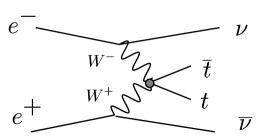
Figure 1: Diagrams for $e^{-}e^{+}\rightarrow\nu{\overline{\nu}}t\bar{t}$ through anomalous  $W^{+}W^{-}t{\bar{t}}\;$ couplings.

As this process also appears in the Higgsless SM, what we hope to observe is actually an interference between the diagrams containing the anomalous couplings and those from Higgsless SM. Let us analyze the latter for the moment, and then examine the effects of the  $W^{+}W^{-}t{\bar{t}}\;$ operators in Section 3.2.

3.1 $t\bar{t}$ with missing $p_{T_{(t\bar{t})}}$ in the Higgsless SM

The Higgsless SM prediction for the process $e^{+}e^{-}\rightarrow t{\bar{t}}\,$ with missing $p_{T_{(t\bar{t})}}$ consists dominantly of two subprocesses: one in which the missing $p_{T_{(t\bar{t})}}$ is carried by two neutrinos, and the other where it is carried by a particle (i.e., a hard photon) which escapes detection.

In the Higgsless SM there are 19 tree level diagrams for the process $e^{-}e^{+}\rightarrow\nu{\overline{\nu}}t\bar{t}$. There are three $W^{+}W^{-}$ fusion diagrams which, at high energies are the most important contributions, along with six $W$ exchange diagrams of a lower magnitude [cf. Fig. 2(a) and (b) respectively]. (These nine diagrams form a gauge invariant subset). The set of 10 diagrams in Fig. 2(c) contribute to less than about one percent of the total $t{\bar{t}}\nu{\bar{\nu}}$ rate after imposing the kinematic cuts (cf. Eq. (4)) for suppressing the $\gamma t\bar{t}$ background.

Since our signal consists of a $t\bar{t}$ pair with missing transverse momentum (carried by the neutrinos), we also must consider the background process (at order $\alpha_{em}^{2}$) $e^{-}e^{+}\rightarrow\gamma t\bar{t}$ [cf. Fig. 3], where the photon escapes the range covered by the detector, but is sufficiently hard to generate the required missing $p_{T_{(t\bar{t})}}$. The pictured diagrams correspond to initial state radiation (ISR). There are also contributions due to final state radiation (FSR), where a photon is radiated from the $t$ or $\bar{t}$ in the final state, but these contributions are suppressed by the heavy top mass and thus provide a negligible effect.

Figure 2: Representative diagrams for Higgsless SM $e^{-}e^{+}\rightarrow\nu{\overline{\nu}}t\bar{t}$: (a) $W^{+}W^{-}$ fusion, (b) $W$ exchange, and (c) $e^{-}e^{+}$ anihilation.

Figure 3: Diagrams for the ISR subprocess, $e^{-}e^{+}\rightarrow\gamma t\bar{t}\;$.

Using a Monte-Carlo program to calculate the total cross section for the $e^{-}e^{+}\rightarrow\nu{\overline{\nu}}t\bar{t}$ process, we compare the results with the ones obtained in Ref. [6], in which the effective $W$ approximation method was applied and a total cross section $\sigma_{{W^{+}}_{L}{W^{-}}_{L}\rightarrow t\bar{t}}=2$ fb was obtained. In that calculation only the longitudinal components of the massive $W$ bosons were considered, as well as the leading terms in powers of $E$ for the helicity amplitudes ${W^{+}}_{L}{W^{-}}_{L}\rightarrow t\bar{t}$. By applying the same requirements as used in the effective $W$ study, we can compare our exact calculations to see how well the effective $W$ approximation works in this process. Namely, we require the invariant mass of the $t\bar{t}$ system to be $M_{t\bar{t}}>500$ GeV and the rapidity and the transverse momentum of $t$ and $\bar{t}$ to be $|y|\leq 2$ and $p_{T}\geq 20$ GeV, respectively. From the complete matrix element calculation, we obtain a similar value of 2.2 fb for the total cross section. Comparing this with the $2$ fb obtained from the effective $W$ approximation, we conclude that the effective $W$ approximation provides an accurate estimate of the total cross section in this kinematic region to about 10%.

In order to suppress the background from the ISR subprocess of $e^{+}e^{-}\rightarrow\gamma t\bar{t}$, we have found it essential to require that the $t\bar{t}$ system have a minimum of transverse momentum, $p_{T_{(t\bar{t})}}\geq 20$ GeV. Because this ISR subprocess dominantly produces photons approximately co-linear with the beam axis, this constraint will remove much of the background. Any photon with polar angle $\theta$ less than 0.15 rad and energy more than $20/0.15\simeq 130$ GeV will not be removed by this cut. Roughly speaking, only $10\%$ of the initial state radiation carries this (or more) energy [13]. Thus we are effectively cutting out most of the ISR background, which nonetheless remains the order of the $W^{+}W^{-}$ fusion Higgsless SM cross section ($\sigma_{\gamma t\bar{t}}=1.8$ fb).

After imposing the minimal set of constraints:

$$|y_{t}|,\,|y_{\bar{t}}|\, \leq 2\,,$$

$$p_{T_{(t)}},p_{T_{(\bar{t})}} \geq 20\,{\rm GeV}\,,$$

$$p_{T_{(t\bar{t})}} \geq 20\,{\rm GeV},$$ (4)

we find that the cross section for $e^{+}e^{-}\rightarrow\nu{\bar{\nu}}t\bar{t}$ is about 4.0 fb in the Higgsless SM. This indicates that the effective $W$ approximation used in [6] estimated the total rate for $t\bar{t}$ production via $W^{+}W^{-}$ fusion at the LC by about a factor of 2 too small . However, as we shall show, this will not have a large effect on the limits which can be obtained on $a_{1,2}$ by studying the total rate for $t\bar{t}$ with missing $p_{T_{(t\bar{t})}}$ at the LC, particularly when the ISR contribution to the background is included.

The two type of processes, $\nu{\bar{\nu}}t\bar{t}$ by $W^{+}W^{-}$ fusion, and $\gamma t\bar{t}$ by $e^{+}e^{-}$ anihilation, have different distributions in several kinematical variables. For instance, in Fig. 4 we show the rapidity ($y_{t\bar{t}}$) of the $t\bar{t}$ system for each subprocess. For the ISR process, which is a two-to-three process, the rapidity has a minimum absolute value of about 0.18; this means that the $t\bar{t}$ pair must have a minimum thrust toward the beam axis. This can be easily understood from the fact that the emitted photon, which must be directed close to the beam axis in order to escape detection, must carry enough energy in order to generate the required missing $p_{T_{(t\bar{t})}}$, and consequently the $t\bar{t}$ system is boosted. On the other hand, the $W^{+}W^{-}$ fusion mechanism prefers the $t$ and $\bar{t}$ to be produced in the rapidity region close to zero.

Figure 4: Distribution of $y_{t\bar{t}}$ for Higgsless SM $e^{-}e^{+}\rightarrow\nu{\overline{\nu}}t\bar{t}$ (upper curve), and for $e^{-}e^{+}\rightarrow\gamma t\bar{t}$ (lower curve).

Another important difference between these processes is their dependence on the polarization of the initial electron and positron beams. For $W^{+}W^{-}$ fusion the only non-zero contribution comes from a purely left-handed electron and a purely right-handed positron. The rate for polarized $e^{+}$ or $e^{-}$ beams can be written in terms of the rate for unpolarized beams by using the relation,

$$\sigma_{e^{-}e^{+}\rightarrow\nu{\overline{\nu}}t\bar{t}}\,=\,\sigma^{(0)}_{e^{-}e^{+}\rightarrow\nu{\overline{\nu}}t\bar{t}}\times(1+P^{-}_{e^{-}})\times(1+P^{+}_{e^{+}})$$ (5)

where $\sigma^{(0)}_{e^{-}e^{+}\rightarrow\nu{\overline{\nu}}t\bar{t}}$ is the unpolarized beam rate (determined to be 4 fb after imposing the minimal cuts described above), and $P^{-}_{e^{-}}$ ($P^{+}_{e^{+}}$) are the fractional left (right) polarization of the electron (positron) beams respectively. On the other hand, for $t\bar{t}\gamma$ production the vector coupling also allows for contribution from a right (left) handed electron (positron). Therefore, to enhance the signal-to-background ratio we should consider the possibility of enhancing the $W^{+}W^{-}$ fusion with an $e^{-}$ ($e^{+}$) beam with some degree of left (right) handed polarization. In Fig. 5 we show the ratio of the total cross sections of these two processes as a function of the left-handed polarization of the electron beam, and for three different values of right-handed polarization of the positron beam.

Figure 5: Ratio of $\sigma_{e^{-}e^{+}\rightarrow t\bar{t}\gamma}$ and $\sigma_{e^{-}e^{+}\rightarrow\nu{\overline{\nu}}t\bar{t}}$ as a function of the left handed polarization of the electron beam and for three different values of $P^{+}_{e^{+}}$ right handed polarization of the positron beam: 0, 0.5 and 1 for the upper, middle and lower curves respectively.

Apart from the expected reduction of $\sigma_{e^{-}e^{+}\rightarrow t\bar{t}\gamma}$ relative to the size of $\sigma_{e^{-}e^{+}\rightarrow\nu{\overline{\nu}}t\bar{t}}$ for higher degrees of polarization, there are two things that can be noticed from Fig. 5. First, for higher degrees of (left-handed) polarization of the electron beam there is no substantial reduction in the ratio ${\sigma_{e^{-}e^{+}\rightarrow t\bar{t}\gamma}}/{\sigma_{e^{-}e^{+}\rightarrow\nu{\overline{\nu}}t\bar{t}}}$ if we also increase the positron’s right-handed polarization. Second, for the case of an unpolarized positron beam the rate of reduction of the ratio falls off as one polarizes the electron beam more and more. In other words, there is more progress in the relative reduction of ${\sigma_{e^{-}e^{+}\rightarrow t\bar{t}\gamma}}$ as one sets the electron’s polarization from 0 to 0.5 than from 0.5 to 1.0. As a consequence of this, the best improvements in the bounds of the anomalous couplings $a_{1}$ and $a_{2}$ take place in the lower degrees of polarization (assuming that no significant deviation from the SM prediction is observed). In Fig. 6 we show the improvement of the bounds for $a_{1}$ and $a_{2}$ depending on the polarization of the electron beam (assuming an unpolarized positron beam). From this study we see that an improvement of about 43% for $a_{1}$ and 11% for $a_{2}$ results when one considers the constraint obtained from an unpolarized beam compared to that which is possible from a completely polarized beam. These results lead us to conclude that a polarized electron beam can be an important and useful tool in probing this type of new physics effect at the LC.

Figure 6: Improvement on the upper and lower bounds of $a_{1}$ and $a_{2}$ (solid and dot-dashed lines respectively) for an unpolarized positron beam but a left-handed polarized electron beam.

One more feature that distinguishes the two subprocesses is the polarization of the $t$ and $\bar{t}$ quarks. Should it turn out to be experimentally feasible to measure the polarizations of the $t$ and $\bar{t}$, this information can also be used to separate the two subprocesses. In $W^{+}W^{-}$ fusion we find the parallel helicities (equal sign) final states to dominate over the antiparallel ones. On the other hand, for the ISR sub-process we find that the opposite is true. To illustrate this point, we show in Fig. 7 the contributions to the rapidity distributions from the various $t$ and $\bar{t}$ polarization combinations.

Figure 7: The distribution of $y_{t\bar{t}}$ for Higgsless SM $e^{-}e^{+}\rightarrow\nu{\overline{\nu}}t\bar{t}$ (lower figure), and for $e^{-}e^{+}\rightarrow\gamma t\bar{t}$ (upper figure), for various $t$ and $\bar{t}$ helicities. The solid lines indicate parallel helicities, $t(+){\bar{t}}(+)$ (upper curves) and $t(-){\bar{t}}(-)$ (lower curves). The dashed line shows antiparallel helicities, $t(+){\bar{t}}(-)$. The dotted line represents helicity combination $t(-){\bar{t}}(+)$.

3.2 Effects from the anomalous  $W^{+}W^{-}t{\bar{t}}\;$ couplings

As demonstrated in [6], the anomalous couplings may be discovered or constrained by examining their effect upon the total production rate of $t\bar{t}$ pairs at the LC. In Fig. 8 we show the total number of $W^{+}W^{-}$ fusion events expected at the LC with integrated luminosity $L=200\;{\rm fb}^{-1}$, as a function of the anomalous operator couplings, $a_{1}$ and $a_{2}$. We can use these results to obtain bounds on $a_{1}$ and $a_{2}$ at the 95% C.L., provided no new physics effects are observed at the LC. In Table 1, we present the constraints on $a_{1}$ and $a_{2}$ from the total rate estimated in [6], as well as the more realistic bounds obtained in this work, including the ISR process $t\bar{t}\gamma$ discussed above, and the intrinsic Higssless SM background processes. We find that the two results are in agreement to within a factor of two, though the more realistic estimation does suffer in some cases when the $t\bar{t}\gamma$ background is included.

Figure 8: Number of $W^{+}W^{-}$ fusion $t\bar{t}$ pairs as a function of the anomalous couplings $a_{1}$ (solid line) and $a_{2}$ (dash-dot line). The point $a_{1}=a_{2}=0$ corresponds to the prediction of the Higgsless SM.

However, as we have discussed above, the background from $t\bar{t}\gamma$ has different rapidity distributions from the $W^{+}W^{-}$ fusion process we wish to study. In Figs. 9, 10, and 11 we show that the effects of  $W^{+}W^{-}t{\bar{t}}\;$ operators can modify the shape of these distributions. Thus, by examining the effect on the shape of the rapidity distributions, we find that it is possible to improve the bounds obtained by studying the total cross section. Because the contribution of the scalar operator ($a_{1}$) is largely S-wave, as is the SM contribution, the scalar operator does not have a large effect on the rapidity distributions of $t$, $\bar{t}$, or the $t\bar{t}$ system. Thus we find that the bounds on $a_{1}$ improve only slightly. For the tensor operator (which contributes to the P-wave) we find a larger effect, and there is a significant improvement on the lower constraint on $a_{2}$. In particular, we find that the effect of the tensor operator is to shift the rapidity distribution of the $t$ and $\bar{t}$ in opposite directions [cf. Figs. 9, 10, and 11]. For this reason it is useful to look at the distribution of $y_{t}-y_{\bar{t}}$ in order to constrain $a_{2}$.

Quantity	bounds for $a_{1}$	bounds for $a_{2}$
Events($W^{+}W^{-}\rightarrow t\bar{t}$)	$-0.06\leq a_{1}\leq 0.07$	$-0.56\leq a_{2}\leq 0.24$
Events($e^{+}e^{-}\rightarrow t{\bar{t}}\nu\bar{\nu}$)	$-0.13\leq a_{1}\leq 0.18$	$-0.9\leq a_{2}\leq 0.2$
$\chi^{2}(y_{t\bar{t}})$	$-0.10\leq a_{1}\leq 0.12$	$-0.78\leq a_{2}\leq 0.18$
$\chi^{2}(y_{t}-y_{\bar{t}})$	$-0.18\leq a_{1}\leq 0.3$	$-0.3\leq a_{2}\leq 0.2$

Table 1: The $95\%$ C.L. limits on $a_{1}$ and $a_{2}$ obtained from studying the total $t\bar{t}$ production rate at the LC and from $\chi^{2}$ analysis of the effects on the distributions of $y_{t\bar{t}}$ and $y_{t}-y_{\bar{t}}$.

Figure 9: Distribution of rapidity of $t$ for the Higgsless SM $W^{+}W^{-}$ fusion process, the $t\bar{t}\gamma$ process, and the $W^{+}W^{-}$ fusion process including one value of $a_{1}$ and $a_{2}$. The solid line corresponds to Higgsless SM $e^{-}e^{+}\rightarrow\nu{\overline{\nu}}t\bar{t}$. The dashed line is $e^{-}e^{+}\rightarrow\gamma t\bar{t}$. The dashed-dotted line is $e^{-}e^{+}\rightarrow\nu{\overline{\nu}}t\bar{t}$ with $a_{2}=0.6$ and the dotted line corresponds to $e^{-}e^{+}\rightarrow\nu{\overline{\nu}}t\bar{t}$ with $a_{1}=-0.4$.

Figure 10: Same as Fig. 9, but for $y_{\bar{t}}$.

Figure 11: Same as Fig. 9, but for $y_{t}-y_{\bar{t}}$.

We analyze the $y_{t}-y_{\bar{t}}$ and $y_{t\bar{t}}$ distributions by computing the $\chi^{2}$ deviation between the distribution including the anomalous effects and that predicted by the Higssless SM, according to the formula,

$$\chi^{2}\,=\,\Sigma^{K}_{j=1}\frac{(N^{A}_{j}-N^{SM}_{j})^{2}}{N^{SM}_{j}},$$ (6)

where $K$ is the total number of bins in the histogram, $N^{A}_{j}$ is the number of events in bin $j$ including the anomalous effects, and $N^{SM}_{j}$ is the number of events predicted by the Higgsless SM in bin $j$. We find that given the statistics available at the LC, for the $y_{t\bar{t}}$ analysis it is optimal to use 3 (equally sized) bins in the region $-0.6\leq y_{t\bar{t}}\leq 0.6$, and 4 bins for the $y_{t}-y_{\bar{t}}\;$ analysis (in the region $0\leq y_{t}-y_{\bar{t}}\leq 2$). In Figs. 12 and 13 we show the dependance of $\chi^{2}$ on the size of the anomalous couplings. Carrying through this analysis and extracting the 95% C.L. bounds on $a_{1}$ and $a_{2}$, we find, as expected, that the limits on $a_{1}$ show a small improvement, while the limits on $a_{2}$ may be improved by about a factor of 2 by considering the $y_{t}-y_{\bar{t}}$ distribution. These results are summarized in Table 1.

Figure 12: $\chi^{2}$ function for $y_{t\bar{t}}$ as a function of $a_{1}$ (solid line) and $a_{2}$ (dash-dotted line).

Figure 13: $\chi^{2}$ function for $y_{t}-y_{\bar{t}}$. The solid line shows the $\chi^{2}$ as a function of $a_{1}$, while the dash-dotted line shows $\chi^{2}$ as a function of coupling $a_{2}$.

The $\chi^{2}$ deviation function for $y_{t\bar{t}}$ shows an interesting behavior at positive (negative) values of $a_{1}$ ($a_{2}$). Instead of growing continually for greater values of the anomalous coupling, it turns over at about a value of 0.5 (-0.3), falls to a minimum at 0.85 (-0.6), and then rises again as the anomalous coupling is increased. This can easily be understood from Fig. 8, which shows the total number of events expected as a function of $a_{1}$ and $a_{2}$. Since the shape of the $y_{t\bar{t}}$ distribution for the Higgsless SM and anomalous cases are very similar, the $\chi^{2}$ is largely a measure of the effect of the anomalous couplings on the total production rate. For positive (negative) values of $a_{1}$ ($a_{2}$) the interference between the Higgsless SM and anomalous amplitudes is destructive, and thus the rate diminishes. However, as $a_{1}$ ($a_{2}$) becomes more positive (negative) the anomalous amplitude begins to dominate the Higgsless SM one and the rate returns to the Higgsless SM value, thus causing a local minimum in the $\chi^{2}$ function. As the magnitude of the anomalous coupling continues to rise, the production rate rises monotonically above the Higgsless SM value, and thus the $\chi^{2}$ increases. This feature is generic to any such analysis where the process under study receives both SM and anomalous contributions to the total rate (and thus can interfere at the amplitude level) and the distribution under study does not under-go a large change in shape due to the effect of the anomalous operator.

It may be possible to use the information of the rapidity distributions under consideration to dis-entangle the effects of the two  $W^{+}W^{-}t{\bar{t}}\;$ operators under study. In this way one could identify whether an observed  $W^{+}W^{-}t{\bar{t}}\;$ new physics effect at the LC was due to the scalar operator or the tensor operator in Eq. (1). As we have shown in Fig. 11, the $y_{t}-y_{\bar{t}}$ distribution shape can be considerably modified by the effect of a tensor operator, where-as the scalar operator shows a distribution much more like that predicted by the Higgsless SM. Thus if a signal is observed at the LC, the rapidity distribution can serve to help identify which operator is responsible.

Moreover, there is a correlation between the $\chi^{2}$ analysis and the total production rate. For instance, assume that a there are a total of 1400 events (about 200 greater than the Higgsless SM prediction), then according to Fig. 8 this effect is due to either $a_{1}$ being of order -0.3 or $a_{2}$ being of order 0.5. If $a_{1}=-0.3$ we expect then $\chi^{2}_{y_{t\bar{t}}}$ to be of order $10^{2}$ and $\chi^{2}_{y_{t}-y_{\bar{t}}}$ to be of order 30. On the other hand, if $a_{2}=0.5$ we also expect $\chi^{2}_{y_{t\bar{t}}}$ to be of order $10^{2}$, but $\chi^{2}_{y_{t}-y_{\bar{t}}}$ to be of order $90$ (3 times higher than the other case).

3.3 Polarization of $t$ and $\bar{t}$

Should it prove possible to reconstruct the polarization information of the $t$ and $\bar{t}$ at the LC, we expect that this information could be useful in both improving the bounds on $a_{1,2}$ and in identifying the operator responsible if a new physics signal is observed at the LC.

In Eq. (2) we presented the dependence on the anomalous couplings of the process $W^{+}W^{-}\rightarrow t\bar{t}$ for the four possible polarizations of the $t$ and $\bar{t}$ final state. Since the $t(+)\bar{t}(-)$ and $t(-)\bar{t}(+)$ matrix elements do not depend on $a_{1}$, it could be possible to use their rates to probe $a_{2}$ independently from $a_{1}$. In the full calculation of $e^{+}e^{-}\rightarrow t\bar{t}\nu\bar{\nu}$, we find that this is indeed the case. If a large deviation is observed only for parallel $t\bar{t}$ polarizations ($t(+){\bar{t}}(+)$ or $t(-){\bar{t}}(-)$), with no corresponding effect in the anti-parallel rate, one could thus be sure that the tensor operator, $O_{\sigma{\cal W}{\cal W}}^{(5)}$, is not responsible. As discussed above, the rapidity distribution $y_{t}-y_{\bar{t}}$ could further be used to identify the scalar operator, $O_{g{\cal W}{\cal W}}^{(5)}$, as the source of the deviation.

The total number of events for various $t$ and $\bar{t}$ polarizations at the LC (assuming an integrated luminosity of $L=200\;{\rm fb}^{-1}$) are shown in Fig. 14. As noted above, we see that the $t(+)\bar{t}(-)$ rate is independent of $a_{1}$. Thus, by studying the $t(+)\bar{t}(+)$ rate we find that we can improve the bounds on $a_{1}$ by about a factor of 2 (here, we are considering unpolarized electron and positron beams) [cf. Table 2]. We also find a substantial improvement in the lower bound on $a_{2}$ by studying the $t(+)\bar{t}(-)$ rate, due to the fact that the Higgsless SM contribution to this channel is small, thus making new effects from the tensor operator more prominent.

Figure 14: Number of $t\bar{t}$ pairs of various polarizations at the LC (with $L=200\;{\rm pb}^{-1}$ of data) as a function of the anomalous couplings. The solid line is the number of $t{(+)}{\bar{t}}{(+)}$ produced as a function of $a_{1}$. The long-dashed line is the number of $t{(+)}{\bar{t}}{(-)}$ as a function of $a_{1}$. The short-dashed line is the number of $t{(+)}{\bar{t}}{(+)}$ as a function of the coupling $a_{2}$. The dotted line is the number of $t{(+)}{\bar{t}}{(-)}$ as a function of $a_{2}$.

Quantity	bounds for $a_{1}$	bounds for $a_{2}$
Events($e^{+}e^{-}\rightarrow\nu\bar{\nu}t(+){\bar{t}}(+)$)	$-0.08\leq a_{1}\leq 0.08$	$-0.85\leq a_{2}\leq 0.42$
Events($e^{+}e^{-}\rightarrow\nu\bar{\nu}t(+){\bar{t}}(-)$)	-	$-0.28\leq a_{2}\leq 0.20$
$\chi^{2}(y_{t(+)\bar{t}(+)})$	$-0.08\leq a_{1}\leq 0.08$	$-0.76\leq a_{2}\leq 0.4$
$\chi^{2}(y_{t(+)\bar{t}(-)})$	-	$-0.28\leq a_{2}\leq 0.20$
$\chi^{2}(y_{t(+)}-y_{\bar{t}(+)})$	$-0.15\leq a_{1}\leq 0.15$	$-0.20\leq a_{2}\leq 0.20$
$\chi^{2}(y_{t(+)}-y_{\bar{t}(-)})$	-	$-\leq a_{2}\leq 0.38$

Table 2: The bounds from polarized $t$ and $\bar{t}$ quantities ($95\%$ CL). Since $a_{1}$ is not sensitive to the $t(+)\bar{t}(-)$ production, no bounds on $a_{1}$ are given for that polarization. There is no 95% C.L. lower bound on $a_{2}$ from $y_{t}-y_{\bar{t}}$.

Finally, we combine the $t\bar{t}$ polarization information with the effects upon the shape of the rapidity distributions, $y_{t}-y_{\bar{t}}$ and $y_{t\bar{t}}$, for two separate choices of $t\bar{t}$ polarizations: $t(+)\bar{t}(+)$ and $t(+)\bar{t}(-)$, thus combining all of the (possibly in the case of $t$ polarization) measurable quantities considered in this study. The results for the $\chi^{2}$ functions are presented in Fig. 15 and Fig. 16 respectively. At the 95% C.L., we find that the constraints on $a_{1}$ do not change appreciably, because the scalar operator does not have a large effect on the shape of the rapidity distributions, while those on $a_{2}$ are improved some-what by the $y_{t}-y_{\bar{t}}$ analysis. These results are summarized in Table 2.

Figure 15: $\chi^{2}$ function for $y_{t}-y_{\bar{t}}$ for various $t\bar{t}$ polarizations. The solid line shows $t{(+)}{\bar{t}}{(+)}$ and coupling $a_{1}$. The short-dashed line is $t{(+)}{\bar{t}}{(+)}$ and coupling $a_{2}$. The dotted line shows $t{(+)}{\bar{t}}{(-)}$ as a function of coupling $a_{2}$.

Figure 16: $\chi^{2}$ function for $y_{t\bar{t}}$ for polarizations $t{(+)}{\bar{t}}{(+)}$ as a function of $a_{1}$ (solid line) and $a_{2}$ (short dashed line) and for polarizations $t(+){\bar{t}}(-)$ as a function of $a_{2}$ (dotted line). For coupling $a_{1}$ $\chi^{2}$ values for $t{(+)}{\bar{t}}{(-)}$ are smaller than 1.0.

4 Conclusions

In this paper, we present a complete, realistic calculation of the rate for producing $t\bar{t}$ pairs at the LC, an $e^{+}e^{-}$ collider with $\sqrt{s}=1.5$ TeV and $200\;{\rm fb}^{-1}$ of integrated luminosity. We have considered both $t\bar{t}\nu\bar{\nu}$ and $t\bar{t}\gamma$ production, within the frame-work of the the Higgsless Standard model, an effective theory in which the SU(2$)_{L}\times$ U(1$)_{Y}$ gauge symmetry is realized non-linearly. In order to parameterize the effect of “new physics” coming from a high energy scale, we include the possibility of anomalous dimension five  $W^{+}W^{-}t{\bar{t}}\;$ local operators. We have chosen to focus on a scalar ($O_{g{\cal W}{\cal W}}^{(5)}$) and a tensor ($O_{\sigma{\cal W}{\cal W}}^{(5)})$) operator as representative terms in the effective lagrangian which contribute to scattering amplitudes at energy order $E^{3}$, in the S-wave and P-wave channels respectively. Comparing the rate for $e^{+}e^{-}\rightarrow t\bar{t}\nu\bar{\nu}$ to previous work [6], in which the effective $W$ approximation was used to estimate this rate, we find that the effective $W$ method is in good agreement with the full calculation (to within a factor of 2).

We found that by studying the total production rate, it is possible to constrain a dimension five anomalous scalar  $W^{+}W^{-}t{\bar{t}}\;$ coupling by $-0.13\leq a_{1}\leq 0.18$, and a tensor  $W^{+}W^{-}t{\bar{t}}\;$ coupling by $-0.9\leq a_{2}\leq 0.2$. However, one can hope to improve these bounds by considering the effect of the operators on the rapidity distributions $y_{t\bar{t}}$ and $y_{t}-y_{\bar{t}}\;$ to $-0.10\leq a_{1}\leq$ 0.12 and $-0.3\leq a_{2}\leq$ 0.2. In addition, since the deviations from the Higgsless SM distributions depend on $a_{1}$ and $a_{2}$, we can use the $\chi^{2}$ analysis to decide whether the anomalous effect comes from the scalar coupling, the tensor coupling, or from both.

We have also studied the improvements in constraining $a_{1}$ and $a_{2}$ resulting from a polarized electron and/or positron beam. We find that an improvement of about 43% in the bounds on $a_{1}$ and 11% in the bounds on $a_{2}$ result when the electron beam is 100% polarized, and that no large further improvement is expected if the positron beam is also polarized.

Should it prove experimentally feasible to reconstruct the polarization of the $t$ and $\bar{t}$, we can hope to further improve these bounds. By considering the rapidity distributions of $t(+)\bar{t}(+)$ and $t(+)\bar{t}(-)$ separately, one can hope to achieve the constraints $-0.08\leq a_{1}\leq 0.08$ and $-0.20\leq a_{2}\leq 0.20$. Finally, because the scalar operator does not contribute to the $t(+)\bar{t}(-)$ channel, one can also use measurements of the polarized production rates to determine directly which operator is responsible for an observed new physics effect, should an excess in the $t\bar{t}$ with missing $p_{T_{(t\bar{t})}}$ rate be observed at the LC.

Thus, we conclude that the LC would provide an excellent experiment for probing anomalous  $W^{+}W^{-}t{\bar{t}}\;$ couplings, and thus could provide key information on the details associated with the electroweak symmetry breaking sector, should a light Higgs boson fail to be discovered.

References

-
[1]
F. Abe et al., Phys. Rev. Lett. 73, 225 (1994);
S. Abachi et al.,Phys. Rev. Lett. 72, 2138 (1994);
CDF Collaboration, Phys. Rev. Lett. 74, 2626 (1995);
D0 Collaboration, Phys. Rev. Lett. 74, 2632 (1995);
L. Roberts, to appear in the Proceedings of the 28th International Conference on High Energy Physics, Warsaw, Poland, 1996. -
[2]
R.D. Peccei and X. Zhang, Nucl. Phys. B337, 269 (1990);
R.D. Peccei, S. Peris and X. Zhang, Nucl. Phys. B349, 305 (1990).
-
[3]
R.S. Chivukula, E. Gates, E.H. Simmons and J. Terning,
Phys. Lett. B311, 157 (1993);
R.S. Chivukula, E.H. Simmons and J. Terning, Phys. Lett. B331, 383 (1994). -
[4]
D.O. Carlson, E. Malkawi, C.–P. Yuan, Phys. Lett.
B337 145 (1994);
E. Malkawi and C.–P. Yuan. Phys. Rev. D50, 4462 (1994); and Phys. Rev. D52, 472 (1995);
E. Malkawi, Ph.D. Thesis, Michigan State University, August 1996;
E. Malkawi, T. Tait, C.–P. Yuan, Phys. Lett. B385, 304 (1996). - [5] G.L. Kane, published in Proceedings of the Workshop on High Energy Phenomenology, Mexico City, July 1–10, 1991.
- [6] F. Larios and C.–P. Yuan, Phys. Rev. D55, 7218 (1997).
-
[7]
H.-J. He, Y.-P. Kuang, and C.-P. Yuan,
Phys. Rev. D51, 6463 (1995);
hep-ph/9503359, Published in Proc. International Symposium on Beyond The Standard Model IV, Eds. J.F. Gunion, T. Han, J. Ohnemus, December 13-18, 1994, Tahoe, California, USA. -
[8]
J. Bagger, V. Barger, K. Cheung, J. Gunion, T. Han, G.A.
Ladinsky, R. Rosenfeld, and C.–P. Yuan,
Phys. Rev. D49, 1246 (1994); and D52, 3878
(1995).
V. Barger, J. F. Beacom, K. Cheung, T. Han, Phys. Rev. D50, 6704 (1993).
E. Boos, H.–J. He, W. Kilian, A. Pukhov, C.–P. Yuan, and P.M. Zerwas, DESY-96-256, Aug 1997. -
[9]
H. Georgi, Weak Interactions and Modern Particle Theory
(The Benjamin/Cummings Publishing Company, 1984);
A. Manohar and H. Georgi, Nucl. Phys. B234, 189 (1984). - [10] M. Jacob and G. C. Wick, Ann. Phys. 7, 404 (1959).
- [11] M.S. Chanowitz, M.A. Furman and I. Hinchliffe, Nucl. Phys. B153, 402 (1979).
- [12] M. Peskin and H. Murayama, SLAC-PUB-7149, June 1996.
-
[13]
E.A. Kuraev and V.S. Fadin, Sov. J. Nucl. Phys.
41, 466 (1985).
O. Nicrosini and L. Trentadue, Phys. Lett. B196, 551 (1987); Z. Phys. C39, 479 (1988). - [14] Review of Particle Physics, Physical Review D54, 1 (1996).