Abstract

One particle inclusive cross sections in the target fragmentation region are considered and an explicit calculation is performed in $(\phi^{3})_{6}$ model field theory. The collinear divergences can be correctly absorbed into a parton density and a fragmentation function but the renormalized cross section gets a large logarithmic correction as expected in a two scale regime. We find that the coefficient of such a correction is precisely the scalar DGLAP kernel. Furthermore the consistency of this result with an extended factorization hypothesis is investigated.

PACS 13.85.Ni

1 Introduction

Asymptotic freedom has led to important predictions for hard inclusive hadronic processes in perturbative QCD. The basic tools are factorization theorems [1] together with perturbative evaluation of scaling properties. Nevertheless perturbative QCD has been successfully applied also to various semi-inclusive processes, for which a complete factorization proof is still lacking.

In a deep inelastic semi-inclusive reaction a hadron with momentum $p$ is scattered by a far off shell photon with momentum $q$ ($Q^{2}=-q^{2}\gg\Lambda_{QCD}^{2}$) and from the inclusive final state, a hadron with momentum $p^{\prime}$ is detected. Until some years ago the main interest has been devoted in hadron production in the current fragmentation region, that is in the region in which the momentum transfer $t=-(p-p^{\prime})^{2}$ is of order $Q^{2}$ [2]. In the last few years, after the introduction of fracture functions [3], a novel attention has been payed to the target fragmentation region ($t\ll Q^{2}$) [3, 4, 5]. With the observation of diffractive deep inelastic events at HERA part of this attention has been focused on the limit in which the longitudinal momentum fraction of the observed hadron is close to unity and $t$ is of order $1~{}GeV^{2}$ or less.

In this paper we want to deal with semi-inclusive deep inelastic scattering (DIS) in a rather simplified context, that is we will work in $(\phi^{3})_{6}$. The scalar $(\phi^{3})_{6}$ model share with QCD some important aspect. It is an asymptotically free theory and the Feynman diagrams have the same topology as in QCD. Moreover there are no soft but only collinear divergences and so factorization become simpler to deal with. For this reasons it has been customary, in the past, to face a QCD problem by studying it first in $(\phi^{3})_{6}$ [7, 8, 9, 10, 11].

In $(\phi^{3})_{6}$ one can define as in QCD a scalar parton density and a fragmentation function which obey DGLAP evolution equations [8, 11]. It is in this framework that we are going to calculate here the one particle deep inelastic cross section in the limit $t\ll Q^{2}$. The aim of such a calculation is twofold. On one hand we want to verify that the renormalized one particle cross section gets large $\log Q^{2}/t$ corrections, as one naturally expects in the two scale regime $t\ll Q^{2}$. On the other hand we want to check the consistence of our result with the factorization put forward in Ref.[12].

This paper is organized as follows: in Sect.2 we will recall the result one gets in $(\phi^{3})_{6}$ for inclusive DIS. In Sect. 3 we will perform the calculation of the semi-inclusive cross section. In Sect. 4 we will show how an interpretation in terms of cut vertices can be given. In Sect. 5 we will sketch our conclusions.

2 DIS

As a first step we will focus on the deep inelastic inclusive cross section. We consider the process $p+J(q)\to X$ where $J=\frac{1}{2}\phi^{2}$ is a scalar operator which plays the role of the electromagnetic current. We define as usual

$$Q^{2}=-q^{2}~{}~{}~{}~{}~{}~{}x=\frac{Q^{2}}{2pq}.$$ (2.1)

The structure function is

$$W(x,Q^{2})=\frac{Q^{2}}{2\pi}\int d^{6}ye^{iqy}<\!p|J(y)J(0)|p\!>.$$ (2.2)

Figure 1: Lowest order contribution to the deep inelastic cross section

We want to calculate the parton-current cross section $w(x,Q^{2})$ at $p^{2}=0$ in dimensional regularization ($D=6-2\epsilon$), by retaining only divergent contributions. At Born level we have (see Fig. 1)

$$w_{0}(x,Q^{2})=\frac{Q^{2}}{2\pi}2\pi\delta((p+q)^{2})=\delta(1-x).$$ (2.3)

The first order corrections are shown in Fig. 2 and give

$$w_{1a}(x,Q^{2})=\frac{\lambda^{2}}{(4\pi)^{3}}x(1-x)\left(-\frac{1}{\epsilon}\right)\left(\frac{4\pi\mu^{2}}{Q^{2}}\right)^{\epsilon}$$ (2.4)

$$w_{1b}(x,Q^{2})=2\times\frac{1}{2}\frac{\lambda^{2}}{(4\pi)^{3}}\frac{1}{\epsilon}\left(\frac{4\pi\mu^{2}}{Q^{2}}\right)^{\epsilon}\delta(1-x)$$ (2.5)

$$w_{1c}(x,Q^{2})=\frac{1}{12}\frac{\lambda^{2}}{(4\pi)^{3}}\left(-\frac{1}{\epsilon}\right)\left(\frac{4\pi\mu^{2}}{Q^{2}}\right)^{\epsilon}\delta(1-x).$$ (2.6)

The factor $2$ in eq. (2.5) takes into account the contribution from the symmetric diagram. The diagram in Fig.2d gives only a finite correction. External self energies have not be taken into account since we work at $p^{2}=0$.

Figure 2: One loop corrections to the deep inelastic cross section

Usually one has not to worry about current renormalization, because the electromagnetic current is not renormalized by strong interactions. However in our simplified model the operator $J_{0}=\frac{1}{2}\phi_{0}^{2}$ is renormalized by the interaction. The renormalization constant $Z_{J}$ is defined by

$$J=Z_{J}^{-1}J_{0}.$$ (2.7)

We get, in the MS scheme

$$Z_{J}=1+\frac{5}{12}\frac{\lambda^{2}}{(4\pi)^{3}}\frac{1}{\epsilon}.$$ (2.8)

As a matter of fact, being the renormalization scale dependent, the coupling to the current becomes scale dependent, so it turns out more convenient to define a $Q^{2}$ dependent renormalization

$$Z_{J}(Q^{2})=1+\frac{5}{12}\frac{\lambda^{2}}{(4\pi)^{3}}\frac{1}{\epsilon}\left(\frac{4\pi\mu^{2}}{Q^{2}}\right)^{\epsilon}$$ (2.9)

which takes into account this effect. Therefore the cross section is obtained summing up all the contributions and multiplying by $Z_{J}^{-2}(Q^{2})$. Up to finite corrections we get

$$w(x,Q^{2})=\delta(1-x)+\frac{\lambda^{2}}{(4\pi)^{3}}P(x)\left(-\frac{1}{\epsilon}\right)\left(\frac{4\pi\mu^{2}}{Q^{2}}\right)^{\epsilon}$$ (2.10)

where

$$P(x)=x(1-x)-\frac{1}{12}\delta(1-x)$$ (2.11)

is the DGLAP kernel for this model [8, 14]. We see that this result has the same structure one gets in QCD. The contribution to the structure function is obtained as a convolution with the bare parton density $f_{0}(x)$

$$W(x,Q^{2})=\int_{x}^{1}\frac{du}{u}f_{0}(u)w(x/u,Q^{2}).$$ (2.12)

The collinear divergence in $w(x,Q^{2})$ can be absorbed as usual by defining a $Q^{2}$ dependent scalar parton density $f(x,Q^{2})$ by means of the equation

$$f_{0}(x)=\int_{x}^{1}\frac{du}{u}\left[\delta(1-u)+\frac{\lambda^{2}}{(4\pi)^{3}}P(u)\frac{1}{\epsilon}\left(\frac{4\pi\mu^{2}}{Q^{2}}\right)^{\epsilon}\right]f(x/u,Q^{2}).$$ (2.13)

This renormalized scalar parton density obeys the DGLAP evolution equation

$$Q^{2}\frac{\partial}{\partial Q^{2}}f(x,Q^{2})=\int_{x}^{1}\frac{du}{u}P(u)f(x/u,Q^{2}).$$ (2.14)

On the same footing one can define for the process $J(q)\to p+X$ with $q$ timelike a fragmentation function $d(x,Q^{2})$ which obeys the same DGLAP evolution equation. Thanks to the Gribov-Lipatov reciprocity relation [15] at one loop level the timelike DGLAP kernel is the same as in the spacelike case, but this relation is broken at two loop, as explicitly verified for $(\phi^{3})_{6}$ in Ref.[9].

3 Semi-inclusive DIS

We are now ready to discuss the process $p+J(q)\to p^{\prime}+X$. In this case a semi-inclusive structure function can be defined as

$$W(p,p^{\prime},q)=\frac{Q^{2}}{2\pi}\sum_{X}\int d^{6}xe^{iqx}<\!p|J(x)|p^{\prime}X\!><\!Xp^{\prime}|J(0)|p\!>.$$ (3.1)

We define

$$z=\frac{p^{\prime}q}{pq}.$$ (3.2)

We will calculate the partonic cross section in the limit

$$t\ll Q^{2}$$ (3.3)

at leading power, by keeping only divergent terms and possible $\log Q^{2}/t$ contributions. It turns out that the approximation (3.3) selects a special class of diagrams, those in which the produced particle is radiated by the incoming one. As a matter of fact at the lowest order in $\lambda$ there is no contribution in the region $t\ll Q^{2}$. The first diagram is the one in Fig. 3 which gives

Figure 3: Leading order contribution to the one particle deep inelastic cross section in the region $t\ll Q^{2}$

$$w_{1}(x,z,t,Q^{2})=\frac{\lambda_{0}^{2}}{t^{2}}x\delta(1-x-z)$$ (3.4)

where $\lambda_{0}$ is the bare coupling constant. Notice that, at this order it is necessary to distinguish between $\lambda$ and $\lambda_{0}$.

Figure 4: One loop leading contributions to the one particle deep inelastic cross section

Figure 5: One loop finite corrections to the one particle deep inelastic cross section

The other contributions come from the one loop corrections listed in Figs. 4,5. It appears that the topology of the diagrams is much richer than the one for the inclusive scattering. The diagram in Fig. 4(a) gives

$$w_{2a}(x,z,t,Q^{2})=\frac{Q^{2}}{2\pi}\int\frac{d^{D}k}{(2\pi)^{D}}\frac{1}{k^{4}}\frac{1}{(k-p^{\prime})^{4}}\lambda^{4}2\pi\delta_{+}\left((p-k)^{2}\right)2\pi\delta_{+}\left((k-p^{\prime}+q)^{2}\right).$$ (3.5)

We choose as a pair of lightlike vectors $p$ and $q^{\prime}\equiv q+xp$ and set

$$k=\alpha p+\beta q+{\bf k}_{\perp}$$ (3.6)

$$p^{\prime}=\alpha^{\prime}p+\beta^{\prime}q+{\bf p}^{\prime}_{\perp}$$ (3.7)

$$s=2pq.$$ (3.8)

The delta functions can be used to integrate over $\alpha$ and $\beta$. It turns out that the integral over ${\bf k}_{\perp}$ gets the leading contribution in the region of small ${\bf k}_{\perp}^{2}$. In this limit we have

$$w_{2a}(x,z,t,Q^{2})\simeq\frac{1}{2}x(1-x-z)^{3}\lambda^{4}$$

$$\times\int\frac{d^{D-2}{\bf k}_{\perp}}{(2\pi)^{D-1}}\frac{1}{{\bf k}_{\perp}^{4}}\frac{1}{\left((1-z){\bf k}_{\perp}^{2}-2(1-x-z){\bf p}^{\prime}_{\perp}{\bf k}_{\perp}+(1-x-z)(x+z)t\right)^{2}}$$ (3.9)

so there is a collinear divergence at ${\bf k}_{\perp}=0$ which corresponds to the configuration in which $k$ becomes parallel to $p$. The result is

$$w_{2a}(x,z,t,Q^{2})=\frac{\lambda^{2}}{(4\pi)^{3}}\frac{\lambda^{2}}{t^{2}}x\frac{1-x-z}{(x+z)^{2}}\left(-\frac{1}{\epsilon}\right)\left(\frac{4\pi\mu^{2}}{t}\right)^{\epsilon}.$$ (3.10)

In the same way the diagram in Fig. 4(b) has a collinear pole when $k$ gets parallel to $p^{\prime}$ and we get

$$w_{2b}(x,z,t,Q^{2})=\frac{\lambda^{2}}{(4\pi)^{3}}\frac{\lambda^{2}}{t^{2}}x\frac{1-x-z}{(1-x)^{2}}\left(-\frac{1}{\epsilon}\right)\left(\frac{4\pi\mu^{2}}{t}\right)^{\epsilon}.$$ (3.11)

The other calculations are straightforward and give

$$w_{2c}(x,z,t,Q^{2})=\frac{\lambda^{2}}{(4\pi)^{3}}\frac{\lambda^{2}}{t^{2}}\frac{x}{1-z}(1-\frac{x}{1-z})\log\frac{Q^{2}}{t}$$ (3.12)

$$w_{2d}(x,z,t,Q^{2})=\frac{1}{12}\frac{\lambda^{2}}{(4\pi)^{3}}\frac{\lambda^{2}}{t^{2}}x\left(-\frac{1}{\epsilon}\right)\left(\frac{4\pi\mu^{2}}{Q^{2}}\right)^{\epsilon}\delta(1-x-z)$$ (3.13)

$$w_{2e}(x,z,t,Q^{2})=2\times\frac{1}{2}\frac{\lambda^{2}}{(4\pi)^{3}}\frac{\lambda^{2}}{t^{2}}x\left(\frac{1}{\epsilon}\right)\left(\frac{4\pi\mu^{2}}{t}\right)^{\epsilon}\delta(1-x-z)$$ (3.14)

$$w_{2f}(x,z,t,Q^{2})=2\times\frac{1}{2}\frac{\lambda^{2}}{(4\pi)^{3}}\frac{\lambda^{2}}{t^{2}}x\left(\frac{1}{\epsilon}\right)\left(\frac{4\pi\mu^{2}}{Q^{2}}\right)^{\epsilon}\delta(1-x-z)$$ (3.15)

$$w_{2g}(x,z,t,Q^{2})=2\times\frac{1}{12}\frac{\lambda^{2}}{(4\pi)^{3}}\frac{\lambda^{2}}{t^{2}}x\left(-\frac{1}{\epsilon}\right)\left(\frac{4\pi\mu^{2}}{t}\right)^{\epsilon}\delta(1-x-z).$$ (3.16)

Again the factor $2$ in eqs. (3.14)-(3.16) takes into account the contribution of the symmetric diagrams. The diagrams in Fig. 5 are finite and don’t give $\log Q^{2}/t$ contributions so they will be neglected.

There are of course many other diagrams which have not been considered here. They are either diagrams in which the produced particle comes from the fragmentation of the current and diagrams which represent interference between target and current fragmentation. However one can verify immediately that these diagrams are suppressed by powers of $t/Q^{2}$, and so they are not relevant here. For example, consider the diagram depicted in Fig.6(a), in which the observed final state particle comes from current fragmentation. The explicit calculation shows that this diagram is suppressed by two powers of $t/Q^{2}$. This fact can be better understood if we redraw it as in Fig. 6(b): in the large $Q^{2}$ limit there are actually four lines going into a hard vertex and the diagram is suppressed by power counting [12].

Figure 6: (a) A current fragmentation contribution to the semi-inclusive cross section       (b) The same diagram depicted in a different form

Summing up all the contributions, multiplying by $Z_{J}^{-2}(Q^{2})$, introducing the running coupling constant

$$\lambda^{2}(t)=\frac{\lambda^{2}}{1+\beta_{0}\lambda^{2}\log t/4\pi\mu^{2}}\simeq\lambda^{2}\left(1-\frac{3}{4}\frac{1}{(4\pi)^{3}}\lambda^{2}\log\frac{t}{4\pi\mu^{2}}\right)$$ (3.17)

and using

$$\lambda^{2}_{0}=\lambda^{2}\left(1-\frac{3}{4}\frac{\lambda^{2}}{(4\pi)^{3}}\frac{1}{\epsilon}\right)=\lambda^{2}(t)\left(1-\frac{3}{4}\frac{\lambda^{2}}{(4\pi)^{3}}\frac{1}{\epsilon}\left(\frac{4\pi\mu^{2}}{t}\right)^{\epsilon}\right)$$ (3.18)

we finally get

$$w(x,z,t,Q^{2}) =\frac{\lambda^{2}(t)}{t^{2}}x\Big{(}\delta(1-x-z)+\frac{1}{6}\delta(1-x-z)\frac{\lambda^{2}}{(4\pi)^{3}}\frac{1}{\epsilon}\left(\frac{4\pi\mu^{2}}{t}\right)^{\epsilon}$$

$$+\frac{\lambda^{2}}{(4\pi)^{3}}\left(\frac{1-x-z}{(x+z)^{2}}+\frac{1-x-z}{(1-x)^{2}}\right)\left(-\frac{1}{\epsilon}\right)\left(\frac{4\pi\mu^{2}}{t}\right)^{\epsilon}$$

$$+\frac{1}{x}P\left(\frac{x}{1-z}\right)\frac{\lambda^{2}}{(4\pi)^{3}}\log\frac{Q^{2}}{t}\Big{)}.$$ (3.19)

We have now to verify that the collinear divergences in eq. (3) can be correctly absorbed in the redefinition of parton density and fragmentation function. We have

$$W(x,z,t,Q^{2}) =\int_{0}^{1}\frac{du}{u}\int_{0}^{1}\frac{dv}{v^{4}}f_{0}(u)w(up,p^{\prime}/v,q)d_{0}(v)$$

$$=\int_{0}^{1}\frac{du}{u}\int_{0}^{1}\frac{dv}{v^{4}}f_{0}(u)w(x/u,z/uv,tu/v,Q^{2})d_{0}(v).$$ (3.20)

Here the integration measure $dv/v^{4}$ takes into account the scaling of the phase space element of the detected particle.

By using the definition of scale dependent parton density (2.13) and the corresponding definition for fragmentation function, eventually we find

$$W(x,z,t,Q^{2}) =\int_{x+z}^{1}\frac{du}{u}\int_{\frac{z}{u-x}}^{1}\frac{dv}{v^{4}}f(u,t)\frac{\lambda^{2}(t)}{t^{2}}\frac{v^{2}}{u^{2}}\Big{[}\delta\left(1-\frac{x/u}{1-z/uv}\right)$$

$$+\frac{\lambda^{2}}{(4\pi)^{3}}P\left(\frac{x/u}{1-z/uv}\right)\log\frac{Q^{2}}{t}\Big{]}d(v,t)$$ (3.21)

where again only leading $\log Q^{2}/t$ terms have been considered and the integration limits are derived using momentum conservation.

Eq. (3) is our final result. We see that the renormalized hard cross section gets, as expected, a large $\log Q^{2}/t$ corrections whose coefficient is precisely the DGLAP kernel. Such correction, if not properly resummed, can spoil perturbative calculations in the region $t\ll Q^{2}$.

Moreover we find that in the limit $t\to 0$ a new singularity appears in the cross section, which corresponds to the configuration in which $p$ becomes parallel to $p^{\prime}$. As pointed out in Ref.[4], when integrating over $t$, such singularity can’t be absorbed in ordinary parton densities and fragmentation functions and the introduction of a new phenomenological distribution, the fracture function [3] becomes necessary.

Eq. (3) can also be rewritten in the following form (see Fig. 7):

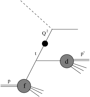
Figure 7: Graphical interpretation of eq. (3)

$$W(x,z,t,Q^{2}) =\frac{\lambda^{2}(t)}{zt^{2}}\int_{x}^{1-z}\frac{dr}{r}\int_{z+r}^{1}\frac{du}{u(u-r)}{\hat{P}}\left(\frac{r}{u}\right)f(u,t)\Big{[}\delta\left(1-\frac{x}{r}\right)$$

$$+\frac{\lambda^{2}}{(4\pi)^{3}}P\left(\frac{x}{r}\right)\log\frac{Q^{2}}{t}\Big{]}d\left(\frac{z}{u-r},t\right)$$ (3.22)

where we have defined the A-P real scalar vertex ${\hat{P}}(x)=x(1-x)$. The function

$$E^{(1)}(x,Q^{2},Q^{2}_{0})=\delta(1-x)+\frac{\lambda^{2}}{(4\pi)^{3}}P(x)\log\frac{Q^{2}}{Q^{2}_{0}}$$ (3.23)

is the first order approximation of the evolution kernel $E(x,Q^{2},Q^{2}_{0})$ which resums the leading logarithmic series [14]. This fact suggests that an interpretation of eq. (3) can be given in terms of Jet Calculus [14].

4 Interpretation in terms of cut vertices

The cut vertex expansion is a generalization of the Wilson expansion originally proposed by Mueller in Ref.[16] and applied to a variety of hard processes in Ref.[17]. We will briefly recall it for DIS in $(\phi^{3})_{6}$.

Let us go back to Sect.2 and set $p^{2}<0$ with $p=(p_{+},{\bf 0},p_{-})$. If we choose a frame in which $p_{+}\gg p_{-}$ we can write for the parton-current cross section [16]

$$w(p,q)=\int\frac{du}{u}v(p^{2},u)C(x/u,Q^{2})$$ (4.1)

where

$$v(p^{2},x)=\int V(p,k)x\delta\left(x-\frac{k_{+}}{p_{+}}\right)\frac{d^{6}k}{(2\pi)^{6}}$$ (4.2)

is a spacelike cut vertex, which fully contains the mass singularities of the cross section, and $C(x,Q^{2})$ is the corresponding coefficient function. In eq. (4.2) $V(p,k)$ is defined as the discontinuity of the four point amplitude in the channel $(p-k)^{2}$ and the integration over $k$ is properly renormalized.

The results of the previous sections can be easily recast in the form of cut vertex expansion. If we define

$$v(x,\epsilon)=\delta(1-x)+\frac{\lambda^{2}}{(4\pi)^{3}}P(x)\left(-\frac{1}{\epsilon}\right)$$ (4.3)

$$C(x,Q^{2})=\delta(1-x)+\frac{\lambda^{2}}{(4\pi)^{3}}P(x)\log\frac{Q^{2}}{4\pi\mu^{2}}$$ (4.4)

we can write eq. (2.10) in the form

$$w(x,Q^{2})=\int_{x}^{1}\frac{du}{u}v(u,\epsilon)C(x/u,Q^{2}).$$ (4.5)

Here $v(x,\epsilon)$ is a spacelike cut vertex defined at $p^{2}=0$ whose mass divergence is regularized dimensionally.

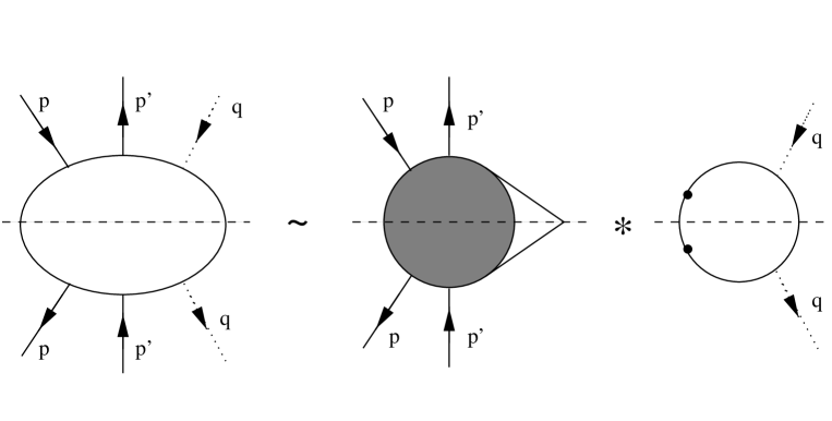
Figure 8: Factorization of the semi-inclusive structure function

It turns out that a similar interpretation can be given of eq. (3). We define

$${\bar{x}}=\frac{x}{1-z}$$ (4.6)

and

$$v({\bar{x}},z,t,\epsilon) =\frac{\lambda^{2}(t)}{t^{2}}\Big{[}\delta(1-{\bar{x}})+P({\bar{x}})\frac{\lambda^{2}}{(4\pi)^{3}}\log\frac{4\pi\mu^{2}}{t}+\frac{\lambda^{2}}{(4\pi)^{3}}\frac{1}{\epsilon}\left(\frac{4\pi\mu^{2}}{t}\right)^{\epsilon}$$

$$\times\left(\frac{1}{6}\delta(1-{\bar{x}})-\frac{(1-z)^{2}{\bar{x}}(1-{\bar{x}})}{({\bar{x}}(1-z)+z)^{2}}-\frac{(1-z)^{2}{\bar{x}}(1-{\bar{x}})}{(1-{\bar{x}}(1-z))^{2}}\right)\Big{]}$$ (4.7)

as a generalized cut vertex [12] which contains all the leading mass singularities of the cross section. We can write up to ${\cal O}(t/Q^{2})$ corrections (see Fig. 8)

$$w({\bar{x}},z,t,Q^{2},\epsilon)=\int_{\bar{x}}^{1}\frac{du}{u}v(u,z,t,\epsilon)C({\bar{x}}/u,Q^{2})$$ (4.8)

where the coefficient function is the same which occurs in inclusive DIS.

It is well known that in dimensional regularization there is a mixing between collinear and ultraviolet divergences. In order to avoid it one should distinguish between $\epsilon$ and $\epsilon^{\prime}$ to regulate UV and collinear divergences, respectively. Moreover external self energies should be taken into account since they are zero on shell for a cancelation of the two kind of divergences. In this framework one can show that factorization (4.8) actually holds graph by graph [19].

5 Conclusions

In this paper we have studied the deep inelastic semi-inclusive cross section in the target fragmentation region and we have performed an explicit calculation in $(\phi^{3})_{6}$ model field theory. We have shown that the renormalized hard cross section gets a large $\log Q^{2}/t$ correction as expected in a two scale regime. Furthermore we have found that the coefficient driving this logarithmic correction is precisely the scalar DGLAP kernel. This result suggests that the $Q^{2}$ dependence of the cross section in such processes at fixed $z$ and $t$ is driven by the same anomalous dimension which controls the inclusive DIS, as proposed in Ref. [12], and in in the context of diffraction in Ref.[6].

We have then examined our result from the point of view of extended factorization and we have found that it is consistent with such an hypothesis. In this framework the partonic semi-inclusive cross section factorizes into a convolution of a new object, a generalized cut vertex $v(p,p^{\prime},{\bar{x}})$ [12], with four rather than two external legs, and a coefficient function $C({\bar{x}},Q^{2})$. The former is of long distance nature and embodies the leading mass singularities of the cross section, while the latter is of perturbative nature and, what is important, it is the same as in inclusive DIS.

Therefore these results verify the validity of the approach proposed in Ref. [12]. Of course the calculation performed here is only a one loop calculation in a scalar model. Nevertheless we believe that the results obtained maintain the same structure in QCD, by assuming in $(\phi^{3})_{6}$ a particularly simple and appealing form.

Acknowledgments

The author would like to thank G. Camici, S. Catani, D.E. Soper and G. Veneziano for useful discussions, and particularly L. Trentadue for his advice and encouragement during the course of this work.

References

• [1] D. Amati, R. Petronzio and G. Veneziano, Nucl. Phys. B140 (1978) 54, B146 (1978) 29; R.K. Ellis, H. Georgi, M. Machacek, H.D. Politzer and G. Ross, Nucl. Phys. B152 (1979) 285.
• [2] G. Altarelli, R.K. Ellis, G. Martinelli, S.Y. Pi, Nucl. Phys. B160 (1979) 301.
• [3] L. Trentadue and G. Veneziano, Phys. Lett. B323 (1994) 201.
• [4] D. Graudenz, Nucl. Phys. B432 (1994) 351.
• [5] D. De Florian and R. Sassot, Phys. Rev. D56 (1997) 426.
• [6] A. Berera and D.E. Soper, Phys. Rev. D53 (1996) 6162; Z. Kunszt and W.J. Stirling, hep-ph/9609245.
• [7] J.C. Taylor, Phys. Lett. B73 (1978) 85.
• [8] Y. Kazama and Y.P. Yao, Phys. Rev. Lett. 41 (1978) 611; Phys. Rev. D19 (1979) 3111.
• [9] T. Kubota, Nucl. Phys. B165 (1980) 277.
• [10] L. Baulieu, E.G. Floratos and C. Kounnas, Phys. Rev. D23 2464 (1981).
• [11] J.Collins, D.E. Soper and G. Sterman in Perturbative QCD ed. by A.H. Mueller (1982) 1.
• [12] M. Grazzini, L. Trentadue and G. Veneziano, to appear.
• [13] J. Collins, Renormalization, Cambridge University Press (1984).
• [14] K. Konishi, A. Ukawa and G. Veneziano, Nucl. Phys. B157 (1979) 45.
• [15] V.N. Gribov and L.N. Lipatov, Phys. Lett. B37 (1971) 78; Sov. J. Nucl. Phys. 15 (1972).
• [16] A.H. Mueller, Phys. Rev. D18 (1978) 3705; Phys. Rep. 73 (1981) 237.
• [17] S. Gupta and A.H. Mueller, Phys. Rev. D20 (1979) 118.
• [18] L. Baulieu, E.G. Floratos and C. Kounnas, Nucl. Phys. B166 (1980) 321.
• [19] M. Grazzini, PHD thesis, in preparation.