SAGA-HE-124-97, SLAC-PUB-7626 Sept. 2, 1997

a) Department of Physics, Saga University

Honjo-1, Saga 840, Japan ^∗

b) Stanford Linear Accelerator Center

Stanford University, Stanford, CA 94309, U.S.A. ^†

 

* Email: kumanos@cc.saga-u.ac.jp, 96td25@edu.cc.saga-u.ac.jp.
 Information on their research is available at http://www.cc.saga-u.ac.jp

/saga-u/riko/physics/quantum1/structure.html.

$\dagger$ Work partially supported by the US Department of Energy under the contract

DE–AC03–76SF00515.

to be published in proceedings by the World Scientific

One and two loop anomalous dimensions
for the chiral-odd structure function $\bf h_{1}$

Because the chiral-odd structure function $h_{1}$ will be measured in the polarized Drell-Yan process, it is important to predict the behavior of $h_{1}$ before the measurement. In order to study the $Q^{2}$ evolution of $h_{1}$, we discuss one and two loop anomalous dimensions which are calculated in the Feynman gauge and minimal subtraction scheme.

1 Introduction

Despite much effort to understand the proton spin structure, we have not reached a consensus in interpreting it in terms of quark and gluon spins. As another way to investigate the proton spin, the transversity distribution $h_{1}$ is proposed. It will be measured in transversely polarized Drell-Yan processes at RHIC. Before the experimental data are taken, we had better predict the behavior of $h_{1}$ as much as we can. Some model estimates on the $x$ dependence have been already done, for example, in the MIT bag model. Furthermore, the leading-order (LO) splitting function and anomalous dimensions were already calculated.$\!{}^{{\bf?}}$ Therefore, rough behavior is already known although they subject to experimental tests.

In these days, the next-to-leading (NLO) analyses are the standard in studying parton distributions not only in the unpolarized ones but also in the longitudinally polarized ones. Hence, it is very important to understand the NLO splitting function or equivalently anomalous dimensions for $h_{1}$. Here, we discuss the one and two loop results, which had been completed recently.$\!{}^{{\bf?}}$ The bare operator is defined by $O_{B}^{n}=\overline{\psi}_{B}Q_{B}^{n}\psi_{B}=Z_{O^{n}}O_{R}^{n}$ with the renormalized one $O_{R}^{n}$. Once the renormalization constant $Z_{O^{n}}$ is determined, the anomalous dimension is calculated by $\gamma_{{}_{O^{n}}}=\mu\,\partial(\ln Z_{O^{n}})/\partial\mu$. We discuss the calculations of $\gamma_{{}_{O^{n}}}$ for chiral-odd operators in the Feynman gauge and minimal subtraction scheme.

2 One-loop anomalous dimensions for $\bf h_{1}$

Because the gluon field does not contribute to the anomalous dimensions directly due to the chiral-odd nature of $h_{1}$, the calculation becomes simpler. In order to study $h_{1}$ in perturbative QCD, we need to introduce a set of local operators ($n=1,2,\cdot\cdot\cdot$)

$$O^{\nu\mu_{1}\cdot\cdot\cdot\mu_{n}}=S_{n}\,\overline{\psi}\,i\,\gamma_{5}\,\sigma^{\nu\mu_{1}}\,iD^{\mu_{2}}\cdot\cdot\cdot iD^{\mu_{n}}\,\psi-\ {\rm trace}\ {\rm terms}\ .$$ (1)

Here, $S_{n}$ symmetrizes the Lorentz indices $\mu_{1}$, …, $\mu_{n}$, and $iD^{\mu}=i\partial^{\mu}+gt^{a}A_{a}^{\mu}$ is the covariant derivative. For calculating the anomalous dimensions of these operators, Feynman rules at the operator vertices should be provided. In order to satisfy the symmetrization condition and to remove the trace terms, the tensor $\Delta_{\mu_{1}}\Delta_{\mu_{2}}\cdot\cdot\cdot\Delta_{\mu_{n}}$ with the constraint $\Delta^{2}=0$ is multiplied. However, the operators in Eq. (1) are associated with one-more Lorentz index $\nu$, so that it is convenient to introduce another vector $\Omega_{\nu}$ with the constraint $\Omega\cdot\Delta$=0. Then, Feynman rules with zero, one, and two gluon vertices become those in Fig. 2.$\!{}^{{\bf?}}$

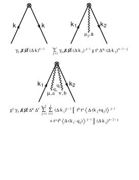
Figure 1: Feynman rules.

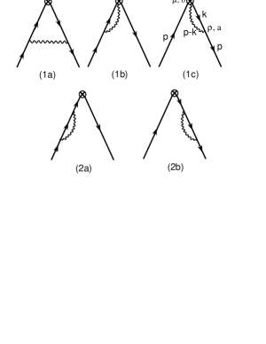
Figure 2: One-loop diagrams.

The one-loop diagrams are shown in Fig. 2. The anomalous dimension $\gamma_{n}$ can be calculated from the $1/\epsilon$ singularity in the dimensional regularization with the dimension $d=4-\epsilon$. Evaluating the diagram (1a), we find that there is no such singularity. It means that there is no contribution to $\gamma_{n}$ from (1a). Obviously, contributions from the diagrams (1b) and (1c) are the same. We show the calculation of the (1c) diagram. With the Feynman rules in Fig. 2, the diagram is evaluated as

$$I_{(1c)} =\int\frac{d^{d}k}{(2\pi)^{d}}\,igt^{a}\gamma^{\rho}\,\frac{ik\!\!\!/}{k^{2}}\,\frac{-ig_{\rho\mu}\delta_{ab}}{(p-k)^{2}}\,\sum_{j=1}^{n-1}\,\gamma_{5}\,\Delta\!\!\!\!/\,\Omega\!\!\!\!/\,(\Delta\cdot p)^{j-1}\,gt^{b}\Delta^{\mu}\,(\Delta\cdot k)^{n-1-j}$$

$$=\gamma_{5}\Delta\!\!\!\!/\,\Omega\!\!\!\!/\,(\Delta\cdot p)^{n-1}\,\biggl{[}-\frac{1}{\epsilon}\frac{4g^{2}}{(4\pi)^{2}}C_{F}\,\left(\frac{-p^{2}}{4\pi}\right)^{-\epsilon/2}\sum_{j=1}^{n-1}\frac{1}{j+1}\biggl{]}\ ,$$ (2)

where $C_{F}$ is given by $C_{F}=(N_{c}^{2}-1)/(2N_{c})$ with the number of color $N_{c}$. From this equation, the diagram (1c) contribution to the anomalous dimension becomes $\gamma_{n}^{(1c)}=\gamma_{n}^{(1b)}=4\,C_{F}\,\sum_{j=1}^{n-1}\,1/(j+1)$. Throughout this paper, we show the anomalous dimension multiplied by the factor $(4\pi)^{2}/g^{2}$ in the one-loop case and $(4\pi)^{4}/g^{4}$ in the two-loop one. Adding all the one-loop contributions in Fig. 2, we obtain $\!{}^{{\bf?}}$

$$\gamma_{n}^{(0)}=2\,C_{F}\biggl{[}\,1+4\,\sum_{j=1}^{n-1}\frac{1}{j+1}\ \biggl{]}\ .$$ (3)

The corresponding LO splitting function is given in Appendix.

3 Two-loop anomalous dimensions

The two-loop anomalous dimensions were calculated recently. $\!{}^{{\bf?}}$ Because the gluon field does not contribute directly, the calculation is similar to the nonsinglet one.$\!{}^{{\bf?}}$ All the two-loop contributions are shown in Figs. 5 and 5.

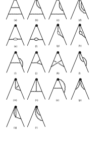
Figure 3: Two-loop contributions.

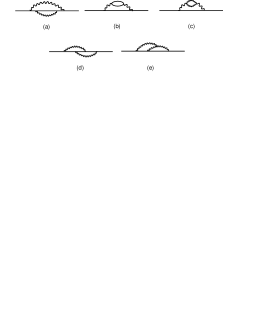
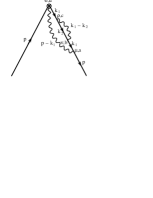
Figure 4: Quark field renormalization.

Figure 5: Lorentz and color indices.

The quark-field renormalization in Fig. 5 was already calculated, so that the problem is to calculate the contributions in Fig. 5. Because it is too complex to explain all the calculations, we discuss only a simple example. The Lorentz and color indices of the diagram (d) in Fig. 5 are shown in Fig. 5, and it is given by

$$I_{(d)}= \int\frac{d^{d}k_{1}}{(2\pi)^{d}}\frac{d^{d}k_{2}}{(2\pi)^{d}}\,igt^{a}\gamma^{\mu}\,\frac{ik\!\!\!/_{1}}{k_{1}^{2}}\,igt^{b}\gamma^{\nu}\,\frac{ik\!\!\!/_{2}}{k_{2}^{2}}\,\frac{-ig_{\nu\rho}\delta_{bc}}{(k_{1}-k_{2})^{2}}\,igt^{c}\gamma^{\rho}\,\frac{ik\!\!\!/_{1}}{k_{1}^{2}}\,\frac{-ig_{\mu\sigma}\delta_{ad}}{(p-k_{1})^{2}}$$

$$\times\,\,\sum_{j=1}^{n-1}\,\gamma_{5}\Delta\!\!\!\!/\,\Omega\!\!\!\!/\,\,(\Delta\cdot p)^{j-1}\,gt^{d}\Delta^{\sigma}\,(\Delta\cdot k_{1})^{n-1-j}\ .$$ (4)

Subtracting a one-loop counter term from the above equation and evaluating singular terms, we have

$$I_{(d)}^{\prime}=\gamma_{5}\Delta\!\!\!\!/\,\Omega\!\!\!\!/\,\,(\Delta\cdot p)^{n-1}\frac{2g^{4}}{(4\pi)^{4}}C_{F}^{2}\sum_{j=1}^{n-1}\frac{1}{j+1}\left[-\frac{2}{\epsilon^{2}}+\frac{1}{\epsilon}\,\{1-S_{1}(j+1)\}\right]\ ,$$ (5)

where $S_{1}(n)=\sum_{k=1}^{n}1/k$. From the above equation, $\gamma_{n}$ becomes $\gamma_{n}^{(d)}=8\,C_{F}^{2}\,[\,G_{1}(n)-S_{1}(n)\,]$ with $G_{1}(n)=\sum_{j=1}^{n}(1/j)\sum_{i=1}^{j}(1/i)$. The factor of two is included by considering a similar diagram with gluons attached to the initial quark line. This result is exactly the same as the unpolarized one in Ref. 3. The reason is the following. Because the operator vertex part $\gamma_{5}\Delta\!\!\!\!/\,\Omega\!\!\!\!/\,$ can be separated from the integrals in Eq. (4), the renormalization constant is independent of the operator form. Therefore, if the gluon lines are attached only to the final-quark or initial-quark line, the anomalous dimensions are the same as those of the unpolarized. In this way, we do not have to repeat the same calculations for the diagrams (d), (g), (h), (l), (m), (q), and (r). The results are listed in Ref. 3. Furthermore, calculating the integrals, we find easily that there is no contribution from the diagrams (a), (b), (c), and (p). The problem reduces to calculations of remaining diagrams (e), (f), (i), (j), (k), (n), and (o). It is tedious to calculate some of these diagrams. Because the calculation is rather lengthy, we do not show each calculation. Adding all the contributions in Figs. 5 and 5, we obtain the final result for the two-loop anomalous dimensions as $\!{}^{{\bf?}}$

$$\gamma_{n}^{(1)}= C_{F}^{2}\,\bigg{[}\,32\,S_{1}(n)\,\{\,S_{2}(n)\,-\,S_{2}^{\prime}(n/2)\,\}\,+\,24\,S_{2}(n)\,-\,8\,S_{3}^{\prime}(n/2)\,+\,64\,\widetilde{S}(n)$$

$$\ \ \ \ \,-\,8\,\frac{1-(-1)^{n}}{n(n+1)}\,-\,3\,\,\bigg{]}+\,C_{F}\,T_{R}\,\bigg{[}\,-\,\frac{160}{9}\,S_{1}(n)\,+\,\frac{32}{3}\,S_{2}(n)\,+\,\frac{4}{3}\,\,\bigg{]}$$

$$+\,C_{F}\,C_{G}\,\bigg{[}\,\frac{536}{9}\,S_{1}(n)\,-\,\frac{88}{3}\,S_{2}(n)\,+\,4\,S_{3}^{\prime}(n/2)\,-\,32\,\hat{S}(n)$$

$$\ \ \ \ -\,16\,S_{1}(n)\,\{\,2S_{2}(n)\,-\,S_{2}^{\prime}(n/2)\,\}\,+\,4\,\frac{1-(-1)^{n}}{n(n+1)}\,-\,\frac{17}{3}\,\,\bigg{]}\ .$$ (6)

The corresponding NLO splitting function is given in Appendix.

4 Conclusion

The two-loop anomalous dimensions had been calculated recently, so that the next-to-leading-order analyses became possible not only for unpolarized and $g_{1}$ structure functions but also for the structure function $h_{1}$.

Appendix: Splitting functions

The LO and NLO splitting functions are $\!{}^{{\bf?}}$

$$\Delta_{T}P_{qq}^{(0)}(x) =C_{F}\left[\frac{2x}{(1-x)_{+}}+\frac{3}{2}\delta(1-x)\right]\ ,$$ (7)

$$\Delta_{T}P_{qq,\pm}^{(1)}(x) \equiv\Delta_{T}P_{qq}^{(1)}(x)\pm\Delta_{T}P_{q\bar{q}}^{(1)}(x)\ ,$$ (8)

$$\Delta_{T}P_{qq}^{(1)}(x) =C_{F}^{2}\Bigg{[}1-x-\left(\frac{3}{2}+2\ln(1-x)\right)\ln x\;\;\delta_{T}P_{qq}^{(0)}(x)$$

$$\!\!\!\!\!\!\!\!\!\!\!\!\!\!\!\!\!\!\!\!\!\!\!\!\!\!\!+\left.\left(\frac{3}{8}-\frac{\pi^{2}}{2}+6\zeta(3)\right)\delta(1-x)\right]+\frac{1}{2}C_{F}N_{C}\bigg{[}-(1-x)$$

$$\!\!\!\!\!\!\!\!\!\!\!\!\!\!\!\!\!\!\!\!\!\!\!\!\!\!\!\left.+\left(\frac{67}{9}+\frac{11}{3}\ln x+\ln^{2}x-\frac{\pi^{2}}{3}\right)\delta_{T}P_{qq}^{(0)}(x)+\left(\frac{17}{12}+\frac{11\pi^{2}}{9}-6\zeta(3)\right)\delta(1-x)\right]$$

$$\!\!\!\!\!\!\!\!\!\!\!\!\!\!\!\!\!\!\!\!\!\!\!\!\!\!\!+\frac{2}{3}C_{F}T_{f}\left[\left(-\ln x-\frac{5}{3}\right)\delta_{T}P_{qq}^{(0)}(x)-\left(\frac{1}{4}+\frac{\pi^{2}}{3}\right)\delta(1-x)\right]\ ,$$ (9)

$$\Delta_{T}P_{q\bar{q}}^{(1)}(x) =C_{F}\left(C_{F}-\frac{1}{2}N_{C}\right)\Bigg{[}-(1-x)+2S_{2}(x)\,\delta_{T}P_{qq}^{(0)}(-x)\Bigg{]}\ ,$$ (10)

where $\delta_{T}P_{qq}^{(0)}(x)=2x/(1-x)_{+}$ and $S_{2}(x)=\int_{x/(1+x)}^{1/(1+x)}dz/z\ln[(1-z)/z]$.

References

References

• [1] X. Artru and M. Mekhfi, Z. Phys. C45 (1990) 669; Y. Koike and K. Tanaka, Phys. Rev. D51 (1995) 6125.
• [2] S. Kumano and M. Miyama, Phys. Rev. D56 (1997) 2504; W. Vogelsang, hep-ph/9706511; A. Hayashigaki, Y. Kanazawa, and Y. Koike, hep-ph/9707208. The NLO evolution results are discussed in Ref. 4.
• [3] E. G. Floratos, D. A. Ross, and C. T. Sachrajda, Nucl. Phys. B129 (1977) 66; B139 (1978) 545.
• [4] S. Scopetta and V. Vento, hep-ph/9707250.