Implications of the Fleischer-Mannel Bound

Abstract

Fleischer and Mannel (FM) have shown that it may become possible to constrain the angle $\gamma$ of the unitarity triangle from measurements of various $B\to\pi K$ decays. This constraint is independent of hadronic uncertainties to the few percent level. We show that, within the Standard Model, the FM bound gives strong constraints on the CKM parameters. In particular, it could predict a well defined sign for $\sin 2\gamma$ and $\sin 2\alpha$. In a class of extensions of the Standard Model, where the New Physics affects only $\Delta B=2$ (and, in particular, not $\Delta B=1$) processes, the FM bound can lead to constraints on CP asymmetries in $B$ decays into final CP eigenstates even if $B-\bar{B}$ mixing is dominated by unknown New Physics. In our analysis, we use a new method to combine in a statistically meaningful way the various measurements that involve CKM parameters.

I Introduction

Fleischer and Mannel [1] have shown that, using the branching ratios of four $B\to\pi K$ decay modes, it is possible to derive a bound on the angle $\gamma$ of the unitarity triangle which, under certain circumstances, is free of hadronic uncertainties. In this work we show that this bound can provide strong constraints on the CKM parameters within the standard model as well as model independent predictions for various CP asymmetries in neutral $B$ decays.

CKM unitarity allows one to describe any $B$ decay amplitudes as a sum of two terms, each with a definite weak phase related to a particular combination of CKM-matrix elements [2]. For $b\to q\bar{q}s$ decays, it is convenient to choose the two terms as $A=A_{c}+A_{u}e^{-i\gamma}e^{i\delta}$, where $A_{c}\propto|V_{cb}V_{cs}|$, $A_{u}\propto|V_{ub}V_{us}|$, $\gamma$ is the CP violating angle of the unitarity triangle [3] and $\delta$ is a CP conserving strong phase. The amplitudes for the relevant $B\to\pi K$ decays are then written as follows:

$$A(B^{0}\to\pi^{-}K^{+})=A_{c}^{0}-A_{u}^{0}e^{i\gamma}e^{i\delta}, A(\bar{B}^{0}\to\pi^{+}K^{-})=A_{c}^{0}-A_{u}^{0}e^{-i\gamma}e^{i\delta},$$ (1)

$$A(B^{+}\to\pi^{+}K^{0})=A_{c}^{+}-A_{u}^{+}e^{i\gamma}e^{i\delta^{\prime}}, A(B^{-}\to\pi^{-}\bar{K}^{0})=A_{c}^{+}-A_{u}^{+}e^{-i\gamma}e^{i\delta^{\prime}},$$ (2)

The following two assumptions are very likely to hold with regard to these four channels:

1. The contributions to $A_{u}$ that do not come from tree-level amplitudes can be neglected [4]. The reason is that the penguin amplitudes contributions to $A_{u}$ are suppressed compared to their contributions to $A_{c}$ by ${\cal O}(|V_{ub}V_{us}|/|V_{tb}V_{ts}|)\sim 0.02$. Then in the charged $B$ decays, which require a $b\to d\bar{d}s$ transition, we can neglect $A_{u}$ while in the neutral $B$ decays, which are mediated by a $b\to u\bar{u}s$ transition, we take into account only the tree-level amplitude $A_{T}$:

$$A_{u}^{+}=0,\ \ \ A_{u}^{0}=A_{T}.$$ (3)

2. The contributions from electroweak penguins can be neglected [4]. Indeed these contributions can be reliably estimated and they are expected to be of ${\cal O}(0.01)$ of the leading contributions. Then $A_{c}$ comes purely from QCD penguin amplitudes $A_{P}$ which, as a result of the $SU(2)$ isospin symmetry of the strong interactions, contribute equally to the charged and neutral $B$ decays:

$$A_{c}^{0}=A_{c}^{+}=A_{P}.$$ (4)

With the two approximations (3) and (4) one gets [1]

$$\Gamma(B_{d}\to\pi^{\mp}K^{\pm}) \equiv {\Gamma(B^{0}\to\pi^{-}K^{+})+\Gamma(\bar{B}^{0}\to\pi^{+}K^{-})\over 2}\propto|A_{P}|^{2}(1-2r\cos\gamma\cos\delta+r^{2}),$$ (5)

$$\Gamma(B^{\pm}\to\pi^{\pm}K) \equiv {\Gamma(B^{+}\to\pi^{+}K^{0})+\Gamma(B^{-}\to\pi^{-}\bar{K}^{0})\over 2}\propto|A_{P}|^{2},$$ (6)

where

$$r\equiv A_{T}/A_{P}.$$ (7)

This leads to

$$R\equiv{\Gamma(B_{d}\to\pi^{\mp}K^{\pm})\over\Gamma(B^{\pm}\to\pi^{\pm}K)}=1-2r\cos\gamma\cos\delta+r^{2}.$$ (8)

It is clear that $R$ can be smaller than 1 only if there is a destructive interference between the penguin and tree contributions in the neutral $B$ decays. This requires that both $\cos\gamma$ and $\cos\delta$ do not vanish. Thus, if $R<1$ we may get some useful information on $\gamma$.

In general, the constraints on $\gamma$ will depend on hadronic physics. In particular, while $R$ is a measurable quantity, $r$ and $\cos\delta$ are hadronic, presently unknown parameters. (We treat $r$ as a free parameter. Estimates based on factorization and on $SU(3)$ relations prefer $r\lesssim 0.5$ [1].) Fortunately, for a given value of $\cos\gamma\cos\delta$, $R$ has a minimum value as a function of $r$. To find this minimum, we solve

$${dR\over dr}=-2\cos\gamma\cos\delta+2r=0,$$ (9)

which leads to $R_{\rm min}=R(r=\cos\gamma\cos\delta)$, namely

$$R\geq 1-\cos^{2}\gamma\cos^{2}\delta.$$ (10)

The Fleischer-Mannel (FM) bound is derived by setting $\cos\delta=1$:

$$\sin^{2}\gamma\leq R.$$ (11)

Note that a similar bound for $\delta$, $\sin^{2}\delta\leq R$, can be obtained. Also note that additional decay modes, such as $B\to\pi K^{*}$ and $B\to\rho K$, can be used for this analysis.

Clearly, the bound (11) is significant only for $R<1$, as explained in [1]. Recent CLEO results [5] give

$$R=0.65\pm 0.40.$$ (12)

Thus, we may be fortunate and indeed have $R<1$. As soon as an upper bound on $R$ below unity is obtained, the limit (11) will give useful constraints in the $\rho-\eta$ plane within the Standard Model and in the $a_{\pi\pi}-a_{\psi K_{S}}$ (the CP asymmetries in $B\to\pi\pi$ and $B\to\psi K_{S}$, respectively) plane for a class of extensions of the Standard Model [10]. We now describe the derivation and significance of these constraints.

II Standard Model Analysis

Within the Standard Model, bounds on the CKM parameters are often presented as constraints on the unitarity triangle in the $\rho-\eta$ plane. In Fig. 1, we show the present bounds from $|V_{cb}|$, $|V_{ub}/V_{cb}|$, $\Delta m_{B_{d}}$, $\varepsilon_{K}$ and $\Delta m_{B_{s}}$ (see the Appendix for a detailed explanation of our method in combining the constraints). The limit (11) translates into an exclusion region in this plane:

$${\eta^{2}\over\rho^{2}+\eta^{2}}\leq R.$$ (13)

Examples of the exclusion regions are shown in Fig. 2. Once the upper bound on $R$ is below 1, a region around $\rho=0$ is excluded. The choice of these examples is based on the following naive scaling arguments. The CLEO result (12) was obtained with about 3.3 fb^-1. By the beginning of the $B$-factories era, CLEO should reach about 10 fb^-1, so a gain of $\sqrt{3}$ on the statistical error is expected. This gives $\sigma_{R}=0.22$ which, for a central value of $R=0.65$, has still only a small effect compared to the allowed region of Fig. 1. After one year of CLEOIII, BaBar and BELLE we could have about 80 fb^-1, so a gain of about a factor of 5 on the error is expected, namely $\sigma_{R}=0.08$.

Another useful presentation is in the $\sin 2\alpha-\sin 2\beta$ plane [11, 12]. The present allowed region at 95% CL is shown in Fig. 3. Since $\sin^{2}\gamma=1$ corresponds to $\sin 2\alpha=\sin 2\beta$, once the upper bound on $R$ is below 1, a region around the $\sin 2\alpha=\sin 2\beta$ line is excluded. Examples of such constraints are depicted in Fig. 4.

We would like to point out two potentially interesting situations which might develop in the future.

First, the combination of a lower bound on $B_{s}-\bar{B}_{s}$ mixing and an upper bound on $R$ may be very powerful in excluding the possibility of a negative $\cos\gamma$. The reason is that the $\Delta m_{B_{s}}/\Delta m_{B_{d}}$ bound puts a lower bound on $\cos\gamma$ while the $R$ bound translates into an upper bound on negative $\cos\gamma$. To see this explicitly, let us define an $SU(3)$ breaking factor

$$R_{SU(3)}=\left({m_{B_{s}}\over m_{B_{d}}}\right)\left({B_{B_{s}}f_{B_{s}}^{2}\over B_{B_{d}}f_{B_{d}}^{2}}\right).$$ (14)

Then, $|V_{td}/V_{ts}|^{2}=R_{SU(3)}(\Delta m_{B_{d}}/\Delta m_{B_{s}})$ gives

$$\cos\gamma\geq{|V_{us}|^{2}+|V_{ub}/V_{cb}|^{2}-R_{SU(3)}(\Delta m_{B_{d}}/\Delta m_{B_{s}})_{\rm max}\over 2|V_{us}||V_{ub}/V_{cb}|}\geq 1.97-{27.5\;{\rm ps}^{-1}\over\Delta m_{B_{s}}},$$ (15)

where we use $|V_{us}|=0.22$, $\Delta m_{B_{d}}<0.481\;$ps^-1 [13], $|V_{ub}/V_{cb}|>0.06$ [14] and $R_{SU(3)}<1.51$ [15] to get the second inequality. On the other hand, the bound (11) gives an upper bound on $\cos\gamma$ if $\cos\gamma$ is negative:

$$\cos\gamma\leq-\sqrt{1-R}\ \ {\rm for}\ \cos\gamma<0.$$ (16)

Eq. (15) implies that if $(\Delta m_{B_{s}})_{\rm min}\geq 14.0\;$ps^-1 is reached, then the $\Delta m_{B_{s}}$ bound by itself will be enough to exclude negative $\cos\gamma$. But for the interesting range between the present 95% CL lower bound [13], $(\Delta m_{B_{s}})_{\rm min}=10.0\;$ps^-1, and $(\Delta m_{B_{s}})_{\rm min}=14.0\;$ps^-1, only the combination with a low enough $R_{\rm max}$ can exclude the negative $\cos\gamma$ range. For example, with $(\Delta m_{B_{s}})_{\rm min}=10.0\;$ps^-1, eq. (15) gives $\cos\gamma\geq-0.78$, while $R\leq 0.39$ allows negative $\cos\gamma$ only below –0.78. The combination of $\Delta m_{B_{s}}\geq 10.0\;$ps^-1 and $R\leq 0.39$ excludes then a negative $\cos\gamma$ and actually allows only $\cos\gamma\geq 0.78$. The $R_{\rm max}$ values required to close the negative $\cos\gamma$ window for various $(\Delta m_{B_{s}})_{\rm min}$ values are given in Table 1. Of course, a stronger lower bound on $|V_{ub}/V_{cb}|$ (above 0.06) and/or a stronger theoretical upper bound on $R_{SU(3)}$ (below 1.51) will make the task of closing the negative $\cos\gamma$ window easier.

$\displaystyle\begin{array}[]{||c||c|c|c|c||}\hline\cr\hline\cr(\Delta m_{B_{s}})_{\rm min}\ \left[{\rm ps}^{-1}\right]&10&11&12&13\\ \hline\cr R_{\rm max}&0.39&0.72&0.90&0.98\\ \hline\cr(\cos\gamma)_{\rm min}&0.78&0.53&0.32&0.15\\ \hline\cr\hline\cr\end{array}$

TABLE I.: Lower bounds on $\Delta m_{B_{s}}$ and upper bounds on $R$ that close the negative $\cos\gamma$ window and the corresponding lower bound on $\cos\gamma$.

Second, the above $\Delta m_{B_{s}}-R$ combination, together with the existing strong constraints on $\beta$, can exclude a positive $\sin 2\alpha$. The bound $|V_{ub}/V_{cb}|\leq 0.10$ gives $\beta<0.15\pi$. Suppose that $R<0.79$ is established and, furthermore, $\Delta m_{B_{s}}$ is known to be large enough that the negative $\cos\gamma$ window is closed (this would happen under these circumstances with $\Delta m_{B_{s}}>11.3\;$ps^-1). Then we will get a lower bound $\cos\gamma>0.46$ which is equivalent to $\gamma<0.35\pi$. Together with the upper bound on $\beta$, we get $\alpha>\pi/2$, namely $\sin 2\alpha<0$.

To summarize: a combination of (i) a range for $|V_{ub}/V_{cb}|$, (ii) a lower bound on $\Delta m_{B_{s}}$, (iii) an upper bound on $R$ and (iv) the information from $\varepsilon_{K}$ that $\eta>0$, might exclude large regions in the $\rho-\eta$ and $\sin 2\alpha-\sin 2\beta$ planes that are presently allowed. An example of the above situations is given in Figs. 2(b) and 4(b) where an improved measurement for $R$ is assumed. We have a clear prediction of $\cos\gamma>0$ (see Fig. 2(b)) and $\sin 2\alpha<0$ (see Fig. 4(b)).

III Beyond the Standard Model

We now turn to a discussion of the implications of the FM bound for theories beyond the Standard Model. If new physics affects the $B\to\pi K$ decay rates of eq. (1), then the resulting bound (11) might be in conflict with other CKM constraints, thus probing this new physics [16]. In this work, we focus on extensions of the Standard Model where the four decay modes (1) are dominated by the Standard Model diagrams. Yet, we allow for large, even dominant, contributions from New Physics to $B-\bar{B}$ mixing and to $\varepsilon_{K}$. This class of models (without any assumptions on New Physics in $B\to\pi K$ decays) was studied in ref. [10]. It was shown there that combining the information from the CP asymmetries in $B\to\psi K_{S}$ ($a_{\psi K_{S}}$) and in $B\to\pi\pi$ ($a_{\pi\pi}$) with the measurement of $|V_{ub}/V_{cb}|$ allows one to reconstruct the unitarity triangle. Obviously, the FM bound can test this construction. But it also gives a completely new aspect in the model independent analysis by predicting correlations between $a_{\pi\pi}$ and $a_{\psi K_{S}}$. In particular, it might forbid regions in the $a_{\psi K_{S}}-a_{\pi\pi}$ plane. No such definite constraint arises from the $|V_{ub}/V_{cb}|$ bound alone, which is the only other CKM constraint that is viable in a large class of models of new physics.

Let us first repeat the basis for the model independent analysis [10]. We study extensions of the Standard Model with arbitrary (within, of course, phenomenological constraints) new physics contributions to $B-\bar{B}$ mixing and to $K-\bar{K}$ mixing. On the other hand, we assume that the following features hold:

  $(i)$

The $\bar{b}\to\bar{c}c\bar{s}$ and $\bar{b}\to\bar{u}u\bar{d}$ decays for $a_{\psi K_{S}}$ and $a_{\pi\pi}$ respectively, as well as the semileptonic $B$ decays for the $|V_{ub}/V_{cb}|$ measurement, are dominated by Standard Model tree level diagrams.

  $(ii)$

Unitarity of the three generation CKM matrix is practically maintained.

Then, it is possible to use the measurements of $a_{\psi K_{S}}$, $a_{\pi\pi}$ and $|V_{ub}/V_{cb}|$ to construct the Unitarity Triangle and, in particular, to determine the angle $\gamma$ up to an eightfold discrete ambiguity [10]. The validity of these ingredients in extensions of the Standard Model was discussed in [10]. An example of model independent constraints in the $\rho-\eta$ plane is shown in Fig. 5(a). The derivation of the allowed regions is explained in the Appendix.

The FM bound provides a constraint on $\gamma$ and therefore is very interesting for a model independent analysis. However, to apply it in this analysis, one has to make one further assumption:

  $(iii)$

The $\bar{b}\to\bar{u}u\bar{s}$ and $\bar{b}\to\bar{d}d\bar{s}$ decays for the $B\to\pi K$ decays of (1) are dominated by Standard Model diagrams.

We emphasize that this assumption holds much less generically than assumption ($i$) above. While ($i$) concerns decays that are dominated by Standard Model tree diagrams, ($iii$) concerns decays that are dominated by $b\to s$ penguin transitions. The latter are suppressed by loop factors and small CKM factors in the Standard Model and thus are more sensitive to New Physics. Calling the analysis below ‘model-independent’ might be somewhat misleading in this sense. Yet, there is a reasonably large class of models where our three assumptions hold while simultaneously allowing for interesting effects in $B-\bar{B}$ mixing. For example, in models with extra down quark singlets, there could be large CP violating contributions to $B-\bar{B}$ mixing [17], while the contributions to $b\to s$ transitions are constrained by the $B\to\mu^{+}\mu^{-}X$ and $B\to\nu\bar{\nu}X$ bounds to be small [18, 19, 20].

To make things clear we state again that the following analysis applies only to models where the three assumptions $(i)-(iii)$ hold. This is only a subclass of the models to which the analysis of [10] applies.

Examining Fig. 5(a), we learn that the FM bound can test the assumptions that underlie the model independent analysis. A very strong upper bound on $\sin^{2}\gamma$ may turn out to be inconsistent with any of the eight solutions for $\gamma$, implying that there is new physics in at least some of the relevant $\Delta B=1$ processes. In other cases the FM bound can be useful in reducing the discrete ambiguity to fourfold. An example of such a situation is given in Fig. 5(b).

The line of thought that stands in the basis of [10] can be taken a step further: if the angle $\gamma$ of the unitarity triangle is known or, at least, constrained by experimental data, then the predictions for the CP asymmetries $a_{\psi K_{S}}$ and $a_{\pi\pi}$ will be correlated.

The $|V_{ub}/V_{cb}|$ measurement does not constrain $\gamma$. Therefore, the analysis of [10] could not predict any correlations between $a_{\psi K_{S}}$ and $a_{\pi\pi}$: the whole plane (between $-1$ and $+1$ for each asymmetry) is allowed. But the FM bound does constrain $\gamma$. Given an angle $\gamma$ of the unitarity triangle, the crucial relation in the model independent analysis of [10] is

$$2\gamma+\arcsin(a_{\psi K_{S}})+\arcsin(a_{\pi\pi})=2\pi({\rm mod}\ 4\pi),$$ (17)

which is translated in a straightforward way to the following relation between $\sin^{2}\gamma$ and the two asymmetries:

$$(a_{\psi K_{S}}+a_{\pi\pi})^{2}+\tan^{2}\gamma(a_{\psi K_{S}}-a_{\pi\pi})^{2}=4\sin^{2}\gamma.$$ (18)

Eq. (18) defines an ellipse in the $a_{\pi\pi}-a_{\psi K_{S}}$ plane. The principal axes are on the diagonals, and the ratio between them is $|\tan\gamma|$.

An upper bound on $\sin^{2}\gamma$, such as (11), excludes then a region in the $a_{\pi\pi}-a_{\psi K_{S}}$ plane. The excluded region is the area between the ellipse and the boundaries of the plane close to the $(+1,+1)$ and $(-1,-1)$ corners. To understand this picture, one can think in the following way: for $\sin^{2}\gamma=0$, eq. (18) gives the diagonal from $(-1,+1)$ to $(+1,-1)$. As $\sin^{2}\gamma$ increases, the diagonal turns into an ellipse with the ratio between the principal axes, $\tan\gamma$, increasing from $0$ to $\infty$. This corresponds to the ellipse deforming within the plane. At $\sin^{2}\gamma=1$, eq. (18) gives the diagonal from $(-1,-1)$ to $(+1,+1)$. If we have a bound $\sin^{2}\gamma<1$, the ellipse in its deformation does not cover the upper-right and lower-left corners. An example of the exclusion regions is shown in Fig. 6.

A very interesting constraint on the allowed CP asymmetries arises in models where a fourth assumption holds:

  $(iv)$

CP violation in the neutral kaon system is dominated by the Standard Model box diagrams. In other words, $\varepsilon_{K}$ is accounted for by the CKM phase.

This is an interesting situation because, in this case, $\varepsilon_{K}$ gives a lower bound on $\sin^{2}\gamma$. This excludes yet another region in the $a_{\pi\pi}-a_{\psi K_{S}}$ plane. The excluded region is the area between the ellipse (18) that corresponds to $(\sin^{2}\gamma)_{\rm min}$ and the boundaries of the plane close to the $(-1,+1)$ and $(+1,-1)$ corners. This should be intuitively clear from our discussion above of the FM bound in this context. Taking $B_{K}<1$, $|V_{cb}|<0.043$ and $|V_{ub}/V_{cb}|<0.10$, the bound from $\varepsilon_{K}$ reads $\sin\gamma>0.3$. (The information that is relevant to correlating the asymmetries through (18) is $\sin^{2}\gamma>0.1$. The fact that $\varepsilon_{K}$ excludes negative $\sin\gamma$ is irrelevant here.)

The combination of upper and lower bounds on $\sin^{2}\gamma$ (for example the FM bound and the $\varepsilon_{K}$ bound) is even more powerful. If neither $\sin^{2}\gamma=1$ nor $\sin^{2}\gamma=0$ are allowed, then the ellipse in its deformation does not reach not only the corners but also the origin $(0,0)$. Consequently, in addition to the areas excluded separately by each of the bounds, also the area around $(0,0)$ that is inside the overlap of the respective ellipses is excluded. An example of the three regions is given in Fig. 6.

In ref. [10], two more possible scenarios were examined:

  $(iv)^{\prime}$

The $K_{L}\to\pi\nu\bar{\nu}$ decay is dominated by the Standard Model diagrams.

  $(iv)^{\prime\prime}$

The ratio $\Delta m_{B_{s}}/\Delta m_{B_{d}}$ corresponds to $R_{SU(3)}|V_{ts}/V_{td}|^{2}$, even though each of the two mixing parameters is affected by new physics.

Each of $(iv$), ($iv)^{\prime}$ and ($iv)^{\prime\prime}$ holds in some class of models. For certain models, more than one of these assumptions might hold. In any case, the important feature for our analysis is that under any of the three assumptions, future measurements might constrain $\sin^{2}\gamma$. Particularly useful will be a lower bound on $\sin^{2}\gamma$ which can be combined with the FM bound as explained above. Such a lower bound exists already for $\varepsilon_{K}$ and can be achieved with a lower bound on $BR(K_{L}\to\pi\nu\bar{\nu})$ or if $\Delta m_{B_{s}}$ is measured. An upper bound on $\sin^{2}\gamma$ from any of these three measurements (or bounds) is also interesting as it will allow an analysis similar to that of the FM bound within the corresponding class of models.

Finally we note that if any other method to measure or constrain $\gamma$ becomes available, and if the relevant processes are dominated by Standard Model contributions in a class of new physics models, then the above analysis could be applied in a similar way. In particular, Atwood, Dunietz and Soni [21] have recently proposed an improvement of the Gronau-Wyler [22, 23, 24] method to measure $\gamma$ via $B\to KD^{0}(\bar{D}^{0})$ decays. The new method is not only theoretically clean but might also be experimentally feasible. The relevant quark transitions are $b\to c\bar{u}s$ and $b\to\bar{c}us$ which are dominated by the Standard Model tree diagrams in many new physics models (see examples in [25]). Similarly, various proposed methods to measure $\gamma$ through $B_{s}$ decays (see e.g. [26]) can be subject to a similar analysis.

IV Summary

Fleischer and Mannel have suggested a method which, under certain circumstances, can give an upper bound on $\sin^{2}\gamma$ that is almost free of hadronic uncertainties. We have shown that within the Standard Model such a bound can give strong constraints on the unitarity triangle. While at present the information from $\varepsilon_{K}$, $\Delta m_{B_{d}}$ and $|V_{ub}/V_{cb}|$ constrains only $\beta$ to be within one quadrant, the addition of the FM and $\Delta m_{B_{s}}$ bounds can potentially constrain each of $\gamma$ and $\alpha$ to a single quadrant. In particular, if $\sin 2\alpha<0$, this can be deduced from improved FM and $\Delta m_{B_{s}}$ bounds (while currently $\sin 2\alpha$ can assume any value).

In extensions of the Standard Model where the New Physics contributes significantly to $B-\bar{B}$ mixing but to none of the relevant decay processes, the FM bound can give correlations between the allowed values of the CP asymmetries in $B\to\psi K_{S}$ and $B\to\pi\pi$. If also a lower bound on $\sin^{2}\gamma$ is available, for example in models where $\varepsilon_{K}$ is dominated by the Standard Model, the excluded region for these asymmetries is very significant.

A Fitting the CKM Parameters

1 Description of the Basic Method

We explain here our method of statistically combining many measurements involving CKM parameters [27]. The method described below was adopted by the BaBar collaboration [28]. In this work, we combine existing measurements of $|V_{cb}|$, $|V_{ub}/V_{cb}|$, $\Delta m_{B_{d}}$, $\varepsilon_{K}$, and (the lower bound on) $\Delta m_{B_{s}}$ with future measurements of the ratio $R$ defined in eq. (8).

There are two types of errors which enter the determination of the CKM parameters: experimental errors and uncertainties due to theoretical model dependence. These two types of errors will be treated differently.

Experimental errors are generally assumed to be Gaussianly distributed and can then enter a $\chi^{2}$ test. In the following they will be denoted by $\sigma_{cb}$, $\sigma_{ub}$, $\sigma_{\Delta m}$, $\sigma_{\epsilon}$, $\sigma_{\cal A}$ and $\sigma_{R}$ in an obvious notation. (The $\sigma_{\cal A}$ error is related to the $\Delta m_{B_{s}}$ bound and is discussed separately below.) For the quantities with Gaussian errors, we use [13, 14]

$$|V_{cb}| = 0.039\pm 0.004,$$ (A1)

$$|V_{ub}/V_{cb}|_{\rm exp} = |V_{ub}/V_{cb}|_{T}\pm 0.05,$$ (A2)

$$\Delta m_{B_{d}} = 0.463\pm 0.018\ {\mbox{ps}}^{-1},$$ (A3)

$$|\varepsilon_{K}| = (2.258\pm 0.018)\times 10^{-3}.$$ (A4)

$|V_{ub}/V_{cb}|_{T}$ is a central value, defined below. (We actually use yet another parameter in the fit, that is the top mass $\bar{m}_{t}$, with the constraint $\bar{m}_{t}=165\pm 8~{}GeV$.)

A large part of the uncertainty in translating the experimental observables to the CKM parameters comes, however, from errors related to the use of hadronic models. In our work here these are related to the value of $|V_{ub}/V_{cb}|_{T}$ (the subscript $T$ implies that we here refer to the hadronic model dependent range for $|V_{ub}/V_{cb}|$ to which an experimental error should be added to give the full uncertainty) and to the parameters $B_{B_{d}}f_{B_{d}}^{2}$ and $B_{K}$ which enter the calculations of $\Delta m_{B}$ and $\varepsilon_{K}$. At present, one cannot assume any shape for the probability density of these quantities (certainly not Gaussian) and include it in the fit. We thus do not assume any shape for these distributions but use a whole set of ‘reasonable’ values for the parameters. Specifically, we scan the ranges

$$0.06\leq|V_{ub}/V_{cb}|_{T} \leq 0.10,$$ (A5)

$$160\leq f_{B_{d}}\sqrt{B_{B_{d}}} \leq 240\ {\mbox{MeV}},$$ (A6)

$$0.6\leq B_{K} \leq 1.0.$$ (A7)

Once a set of values $M=(|V_{ub}/V_{cb}|_{T},f_{B_{d}}\sqrt{B_{B_{d}}},B_{K})$ has been chosen, a classical least-square minimization can be performed to estimate the CKM parameters (we use here the Wolfenstein parameters [29] $A$, $\rho$ and $\eta$), by relating measurements (with Gaussian errors) to theoretical calculations:

$$\chi^{2}_{M}(A,\rho,\eta) = \left({\langle|V_{cb}|\rangle-|V_{cb}|(A)\over\sigma_{cb}}\right)^{2}+\left({|V_{ub}/V_{cb}|_{T}-|V_{ub}/V_{cb}|(\rho,\eta)\over\sigma_{ub}}\right)^{2}$$ (A8)

$$+ \left({\langle\Delta m_{B_{d}}\rangle-\Delta m_{B_{d}}(A,\rho,\eta)\over\sigma_{\Delta m}}\right)^{2}+\left({\langle|\varepsilon_{K}|\rangle-|\varepsilon_{K}|(A,\rho,\eta)\over\sigma_{\epsilon}}\right)^{2},$$ (A9)

where $\langle a\rangle$ denotes the experimental central value of a quantity $a$. To study the $(\rho,\eta)$ estimates obtained from the global fit, we turn to the usual unitarity triangle representation. In this plane we plot the hypercontour of $\chi^{2}=\chi^{2}_{\rm min}+5.99$ corresponding to the 95% CL contour. Sets of values $M$ with a $\chi^{2}$ probability smaller than 0.05 are rejected and not shown in the plots. Note that for each point of the contour a new minimization is performed with respect to all parameters, meaning that this method takes into account the correlations between the plotted parameters and all other ones. The superposition of the contours for each scanned set of values $M$ is shown in our figures together with the fitted estimates of $(\rho,\eta)$.

Also shown are the ‘minimum and maximum limit’ contours obtained from varying coherently all the uncertainties (theoretical uncertainties are varied within the limits of (A5) and experimental errors between $2\sigma$). These last contours are just shown for comparison, since their statistical meaning is not clear.

The $\chi^{2}$ can also be expressed in terms of another set of parameters: $\chi^{2}(A,\sin 2\alpha,\sin 2\beta)$. It is minimized in the same way as before (using the 5% probability cut) and the 95% CL contours are displayed in the ($\sin 2\alpha,\sin 2\beta$) representation. A subtlety that arises in this analysis is that of discrete ambiguities. As a value $\sin 2\phi$ ($\phi=\alpha$ or $\beta$) corresponds to several possible values of $\phi$, there is a fourfold ambiguity in the values of $(\rho,\eta)$ that correspond to a given pair of values ($\sin 2\alpha,\sin 2\beta$). All four possibilities have to be considered in the fit. In practice, two of them are always incompatible with present data and consequently rejected by the $P(\chi^{2})>0.05$ cut.

2 Including $\Delta m_{B_{s}}$ Properly

The mass difference in the $B_{s}$ system has not been measured and only 95% CL limits have been obtained. Such a limit is only a small part of the information and it cannot be included directly in the $\chi^{2}$ minimization. These problems have been overcome by the amplitude method that is now being used by the LEP $\Delta m_{B_{s}}$ averaging Working Group [13].

For an initially ($t=0$) produced pure $B_{s}$, the probability of a $\bar{B}_{s}$-tagging decay at time $t$ is

$${\cal P}_{m}={1\over 2\tau}e^{-t/\tau}(1-\cos\Delta m_{B_{s}}t),$$ (A10)

while that of a $B_{s}$-tagging decay at time $t$ is

$${\cal P}_{u}={1\over 2\tau}e^{-t/\tau}(1+\cos\Delta m_{B_{s}}t).$$ (A11)

($\tau$ is the $B_{s}$ lifetime.) The amplitude method assumes that the probabilities are described by

$${\cal P}_{m,u}={1\over 2\tau}e^{-t/\tau}(1\pm{\cal A}\cos\Delta m_{B_{s}}t).$$ (A12)

Then, for each value of $\Delta m_{B_{s}}$, ${\cal A}$ and its uncertainty $\sigma_{\cal A}$ are obtained. If ${\cal A}$ is compatible with 0, there is no visible oscillation at this frequency. If ${\cal A}$ were compatible with 1, an oscillation would be observed at this frequency. The 95% CL on $\Delta m_{B_{s}}$ is set at the frequency for which ${\cal A}+1.645\sigma_{\cal A}=1$.

To include this information in our fit, we calculate $\Delta m_{B_{s}}$ for each set of the free parameters $(A,\rho,\eta)$ and find the corresponding measured values of ${\cal A}$ and $\sigma_{\cal A}$. This amplitude is then compared to the one expected if the tested value of $\Delta m_{B_{s}}$ was the correct one (${\cal A}=1)$ and the global $\chi^{2}$ is modified by adding

$$\left({{\cal A}-1\over\sigma_{\cal A}}\right)^{2}$$ (A13)

to the right hand side of eq. (A8).

3 Adding the FM Bound

The FM bound is different from the other constraints that we use, in that experiments give a measurement (see (12)) but the clean information is only an upper bound (see (11)). The way we implement this in our fit (based on a Maximum Likelihood analysis) is the following. Suppose that the experimental result is $R=\langle R\rangle\pm\sigma_{R}$. Then we add to the to $\chi^{2}(A,\rho,\eta)$ a term of the form :

$$0\ \ \ {\rm if} \ \ \ \sin^{2}\gamma(\rho,\eta)<\langle R\rangle,$$ (A14)

$$\left({\sin^{2}\gamma(\rho,\eta)-\langle R\rangle\over\sigma_{R}}\right)^{2}\ \ \ {\rm if} \ \ \ \sin^{2}\gamma(\rho,\eta)>\langle R\rangle.$$ (A15)

We also draw in the figures the two lines corresponding to 95% CL exclusion region which, for one-sided error, are given by $\sin^{2}\gamma=R+1.645\sigma_{R}$.

4 Including New Physics

In the model independent analysis, New Physics effects can be parameterized by 2 new parameters: $r_{d},\theta_{d}$. The theoretical calculations of $\Delta B=2$ processes are to be modified accordingly [10]:

$$\Delta m_{B_{d}}^{NP}(A,\rho,\eta,r_{d})=r_{d}^{2}\Delta m_{B_{d}}^{SM}(A,\rho,\eta)$$ (A16)

$$a_{\psi K_{S}}(A,\rho,\eta,\theta_{d})=\sin 2(\beta(\rho,\eta)+\theta_{d})$$ (A17)

$$a_{\pi\pi}(A,\rho,\eta,\theta_{d})=\sin 2(\alpha(\rho,\eta)-\theta_{d})$$ (A18)

The full $\chi^{2}$ can then be written in terms of all the unknown parameters, once enough measurements are available:

$$\chi^{2}_{M}(A,\rho,\eta,r_{d},\theta_{d}) = \left({\langle|V_{cb}|\rangle-|V_{cb}|(A)\over\sigma_{cb}}\right)^{2}+\left({|V_{ub}/V_{cb}|_{T}-|V_{ub}/V_{cb}|(\rho,\eta)\over\sigma_{ub}}\right)^{2}$$ (A19)

$$+ \left({\langle\Delta m_{B_{d}}\rangle-\Delta m_{B_{d}}^{NP}(A,\rho,\eta,r_{d})\over\sigma_{\Delta m}}\right)^{2}$$ (A20)

$$+ \left({\langle a_{\psi K_{S}}\rangle-a_{\psi K_{S}}(A,\rho,\eta,\theta_{d})\over\sigma_{a_{\psi K_{S}}}}\right)^{2}+\left({\langle a_{\pi\pi}\rangle-a_{\pi\pi}(A,\rho,\eta,\theta_{d})\over\sigma_{a_{\pi\pi}}}\right)^{2}.$$ (A21)

In this case there is no extra degree of freedom to perform a $\chi^{2}$ probability test, but the minimization can be performed and contours can be obtained.

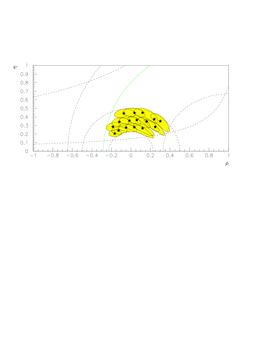
FIG. 1.: The present allowed region for the Unitarity Triangle in the $\rho-\eta$ plane. The input values and the method used for this determination are given in the Appendix.

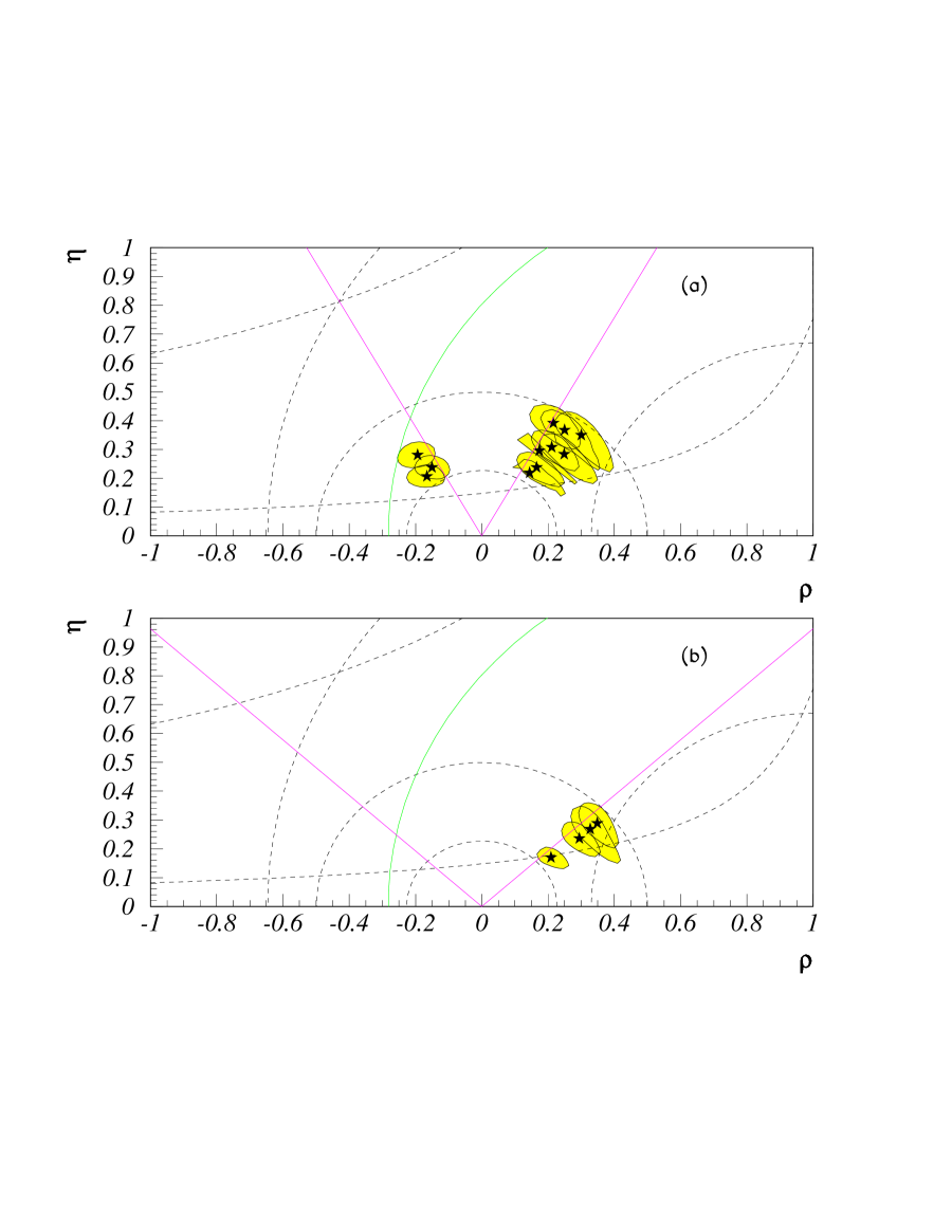
FIG. 2.: The allowed range for the Unitarity Triangle for $(a)$ $R=0.65\pm 0.08$, $(b)$ $R=0.35\pm 0.08$. For all other constraints we use present data.

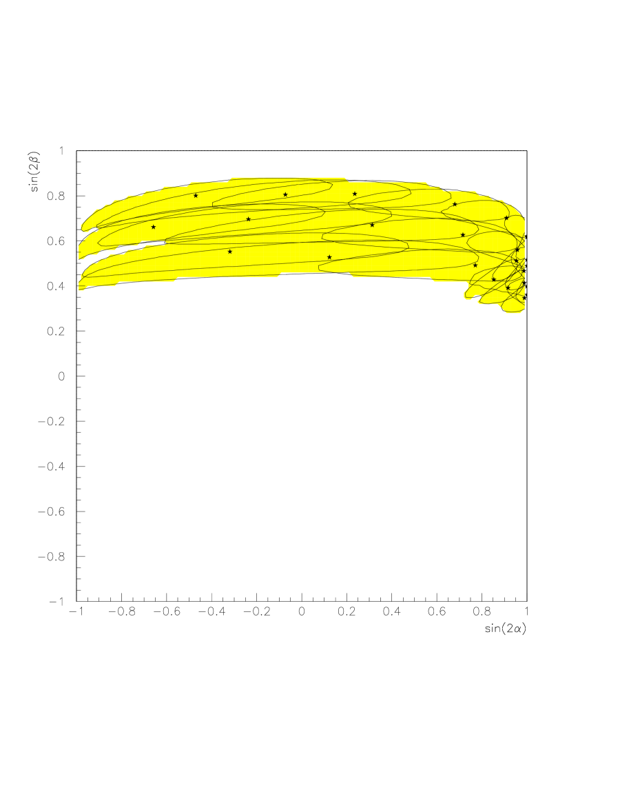
FIG. 3.: The present allowed region in the $\sin 2\alpha-\sin 2\beta$ plane. The input values and the method used for this determination are given in the Appendix.

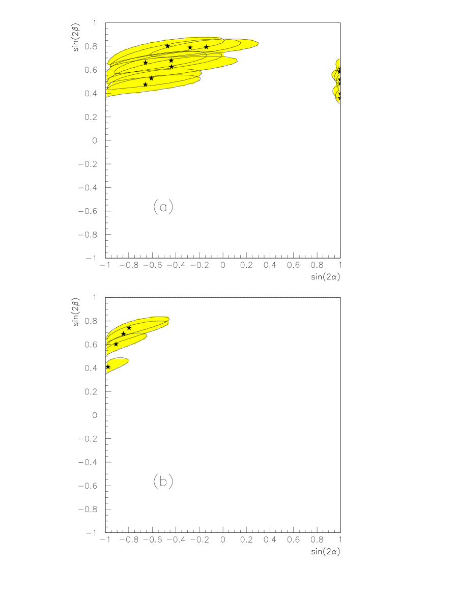
FIG. 4.: The allowed range in $\sin 2\alpha-\sin 2\beta$ plane for $(a)$ $R=0.65\pm 0.08$, $(b)$ $R=0.35\pm 0.08$. For all other constraints we use present data.

FIG. 5.: The model independent construction of the Unitarity Triangle $(a)$ without the FM bound and $(b)$ with $R=0.35\pm 0.08$. We use the current range for $|V_{ub}/V_{cb}|$, $a_{\pi\pi}=0.60\pm 0.09$ and $a_{\psi K_{S}}=0.20\pm 0.06$.

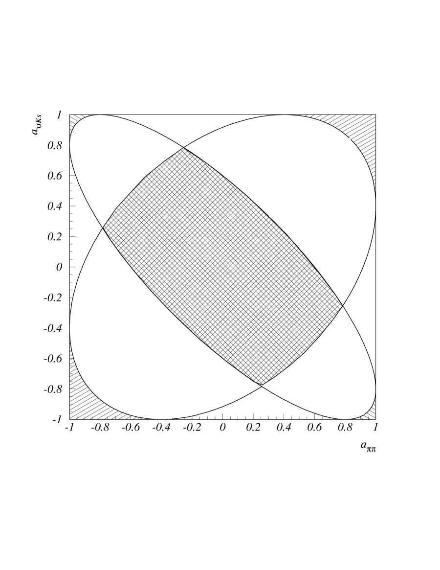
FIG. 6.: The allowed range in the $a_{\pi\pi}-a_{\psi K_{S}}$ plane with New Physics satisfying the conditions specified in the text. The right-hatched area is excluded by an upper bound $\sin^{2}\gamma<0.7$. The left-hatched area is excluded by a lower bound $\sin^{2}\gamma>0.1$. For the combined bound, $0.1<\sin^{2}\gamma<0.7$, the cross-hatched area is also excluded.

REFERENCES

- [1] R. Fleischer and T. Mannel, hep-ph/9704423.
- [2] Y. Grossman and H.R. Quinn, hep-ph/9705356.
- [3] For a review see e.g. Y. Nir and H.R. Quinn, Ann. Rev. Nucl. Part. Sci. 42 (1992) 211.
- [4] For a review see e.g. R. Fleischer, hep-ph/9612446.
- [5] F. Würthwein, the CLEO Collaboration, hep-ex/9706010.
- [6] M. Gronau and D. London, Phys. Rev. Lett. 65 (1990) 3381.
- [7] H.J. Lipkin, Y. Nir, H.R. Quinn and A.E. Snyder, Phys. Rev. D44 (1991) 1454.
- [8] M. Gronau, Phys. Lett. B265 (1991) 389.
- [9] A.E. Snyder and H.R. Quinn, Phys. Rev. D48 (1993) 2139.
- [10] Y. Grossman, Y. Nir and M.P. Worah, hep-ph/9704287.
- [11] J.M. Soares and L. Wolfenstein, Phys. Rev. D47 (1993) 1021.
- [12] Y. Nir and U. Sarid, Phys. Rev. D47 (1993) 2818.
- [13] “Combined Results on Oscillations: Update for the Summer 1997 Conferences”, LEP B Oscillations Working Group, ALEPH 97-083, CDF Internal Note 4297, DELPHI 97-135, L3 Internal Note, OPAL Technical Note TN 502, SLD Physics Note 62.
- [14] R.M. Barnett et al., Particle Data Group, Phys. Rev. D54 (1996) 1.
- [15] C. Sachrajda, a talk presented at the 18th international symposium on lepton – photon interactions, July 28 - August 1, 1997 (Hamburg).
- [16] R. Fleischer and T. Mannel, hep-ph/9706261.
- [17] Y. Nir and D. Silverman, Phys. Rev. D42 (1990) 1477.
- [18] D. Silverman, Phys. Rev. D45 (1992) 1800.
- [19] G. Branco et al., Phys. Rev. D48 (1993) 1167.
- [20] Y. Grossman, Z. Ligeti and E. Nardi, Nucl. Phys. B465 (1996) 369, (E) B480 (1996) 753.
- [21] D. Atwood, I. Dunietz and A. Soni, Phys. Rev. Lett. 78 (1997) 3257.
- [22] M. Gronau and D. London, Phys. Lett. B253 (1991) 483.
- [23] M. Gronau and D. Wyler, Phys. Lett. B265 (1991) 172.
- [24] I. Dunietz, Phys. Lett. B270 (1991) 75; Z. Phys. C56 (1992) 129.
- [25] Y. Grossman and M.P. Worah, Phys. Lett. B395 (1997) 241.
- [26] R. Fleischer and I. Dunietz, Phys. Rev. D55 (1997) 259.
- [27] S. Plaszczynski and M.H. Schune, BaBar Note 340.
- [28] The BaBar Physics Book, SLAC-R-504, in preparation.
- [29] L. Wolfenstein, Phys. Rev. Lett. 51 (1983) 1945.