KEK-TH-537

hep-ph/9709279

November 1997

Abstract
The string theory predicts the unification of the gauge couplings and gravity. The minimal supersymmetric Standard Model, however, gives the unification scale $\sim 2\times 10^{16}$ GeV which is significantly smaller than the string scale $\sim 5\times 10^{17}$ GeV of the weak coupling heterotic string theory. We study the unification scale of the non-supersymmetric minimal Standard Model quantitatively at the two-loop level. We find that the unification scale should be at most $\sim 4\times 10^{16}$ GeV and the desired Kac-Moody level of the hyper-charge coupling should be $1.33~{}{\mathop{<}\limits_{\sim}}~{}k_{Y}~{}{\mathop{<}\limits_{\sim}}~{}1.35$.

The theory of $E_{8}\times E_{8}$ heterotic string [1] has some attractive impacts on the model of low-energy particle physics. The theory has a potential of explaining the low-energy gauge groups, the quantum numbers of quarks, leptons and the Higgs bosons, the number of generations, and the interactions among these light particles which are not dictated by the gauge principle. One of the immediate consequences of the string theory is the unification of the gauge interactions and the gravity. Since, in the string theory, gravitational and gauge interactions are naturally related, the strength of the gauge couplings and the unification scale are both given by the Newton constant. The unification scale of the heterotic string theory is predicted to be [2, 3]

$$m_{U}|_{\rm string}\approx 5\times 10^{17}~{}{\rm GeV},$$ (1)

in the weak coupling limit where the 1-loop string effects are taken into account. On the other hand, the minimal supersymmetric Standard Model (MSSM) predicts the unification scale

$$m_{U}|_{\rm MSSM}\approx 2\times 10^{16}~{}{\rm GeV},$$ (2)

by using the recent results of precision electroweak measurements as inputs. The discrepancy between (1) and (2) is a few percent of the logarithms of these scales. However the extrapolation of (1) to the weak scale leads the experimentally unacceptable values of $\sin^{2}\theta_{W}$ and $\alpha_{s}$ under the hypothesis that the spectrum below the string scale is that of the MSSM. Various attempts to modify this naive prediction are reviewed in ref. [3]. For instance, the 2-loop string effects are not known. On the other hand, it has been suggested [4] that the strong coupling limit of the $E_{8}\times E_{8}$ heterotic string theory, which is considered to be the 11-dimensional M-theory, can give rise to a significantly lower string scale than the estimation (1) in the weak coupling limit.

Alternatively, the gauge coupling unification scale can be modified in string theories with non-standard Kac-Moody levels. The coupling constant $g_{U}$, which is related to the Newton constant in the string theory, is expressed in terms of the SU(3)_C, SU(2)_L and U(1)_Y gauge couplings and the corresponding Kac-Moody level $k_{i}~{}(i=Y,2,3)$ as [5]

$$g_{U}^{2}=k_{i}g_{i}^{2},$$ (3)

at the unification scale $m_{U}$. The factor $k_{i}$ should be positive integer for the non-Abelian gauge group. On the other hand, for the Abelian group, its value depends on the structure of four-dimensional string models. In view of the gauge field theory, $k_{i}$ plays the role of a normalization factor for $g_{i}$ and, for example, the set $(k_{Y},k_{2},k_{3})=(5/3,1,1)$ is taken to embed the hyper-charge $Y$ in the SU(5) GUT group.

It has been known that the SU(5) grand unification is not achieved if one extrapolates the observed three gauge couplings by using the renormalization group equations (RGE) in the minimal Standard Model (SM). It has been noted [3], however, that the trajectories of the SU(2)_L and the SU(3)_C couplings intersect at near the unification scale $m_{U}$ predicted by the string theory: for example, the leading order RGE with a certain choice of the weak mixing angle and the QED coupling in the $\overline{{\rm MS}}$ scheme,

$$\sin^{2}\theta_{W}(m_{Z})_{\overline{{\rm MS}}} = 0.2315,$$ (4a)

$$1/\alpha(m_{Z})_{\overline{{\rm MS}}} = 128,$$ (4b)

gives the following results,

$$m_{U} \approx 1\times 10^{17}~{}{\rm GeV}~{}~{}~{}~{}~{}~{}~{}~{}~{}~{}~{}~{}~{}{\rm for}~{}~{}\alpha_{s}(m_{Z})=0.118,$$ (5a)

$$\approx 2\times 10^{17}~{}{\rm GeV}~{}~{}~{}~{}~{}~{}~{}~{}~{}~{}~{}~{}~{}{\rm for}~{}~{}\alpha_{s}(m_{Z})=0.121.$$ (5b)

The above unification scale $m_{U}$ is remarkably close to the string scale (1), which may suggest the string unification without supersymmetry for the Kac-Moody level $k_{Y}\approx 1.27$ for $k_{2}=k_{3}=1$.

Of course, deserting supersymmetry (SUSY) after compactification into four-dimension means that both the gauge hierarchy and the fine-tuning problems have to be solved without SUSY. The existence of a consistent string theory without the four-dimensional SUSY has not been demonstrated. It has been argued that the solution to these problems, if it exists, should be intimately related to the vanishing of the cosmological constant; see, $e.g.$, ref. [3] for a review of some exploratory investigations. Recently, as an application of this idea of minimal particle contents, the mechanism of baryogenesis in non-SUSY, non-GUT string model has been proposed [6].

In this letter we examine quantitatively at the next-to-leading-order (NLO) level the possibility of the string unification of the gauge couplings in the SM without SUSY. Because, in the string theory, the U(1)_Y coupling can be rather arbitrarily normalized by the Kac-Moody level $k_{Y}$, we define $m_{U}$ as the scale at which the trajectories of the SU(2)_L and the SU(3)_C running couplings intersect with $k_{2}=k_{3}=1$. Our purposes are to find the scale $m_{U}$ and the corresponding $k_{Y}$ under the current experimental and theoretical constraints on the parameters in the minimal SM. In the NLO level, the scale $m_{U}$ is not only affected by the uncertainty in the SU(3)_C coupling but also by threshold corrections due to the SM particles such as the top-quark and the Higgs boson. The top-quark Yukawa coupling affects the RGE at the two-loop level. Therefore, it is interesting to examine whether the scale $m_{U}$ in the minimal SM still lie in the string scale $\sim O(10^{17}~{}{\rm GeV})$ after the NLO effects are taken into account.

We first evaluate quantitatively the U(1)_Y and SU(2)_L $\overline{{\rm MS}}$ couplings at the weak scale boundary of the RGE. The magnitudes of the $\overline{{\rm MS}}$ couplings are determined in general by comparing the perturbative expansions of a certain set of physical observables with the corresponding experimental data. The correspondence can be made manifest by using the effective charges $\bar{e}^{2}(q^{2})$ and $\bar{s}^{2}(q^{2})$ of ref. [7]. The $\overline{{\rm MS}}$ couplings $\hat{\alpha}(\mu)=\hat{e}^{2}(\mu)/4\pi$ and $\hat{\alpha}_{2}(\mu)=\hat{g}_{2}^{2}(\mu)/4\pi$ are related with the effective charges as

$$\frac{1}{\bar{\alpha}(q^{2})} = \frac{1}{\hat{\alpha}(\mu)}+4\pi{\rm Re}\overline{\Pi}^{QQ}_{T,\gamma}(\mu;q^{2}),$$ (6a)

$$\frac{\bar{s}^{2}(q^{2})}{\bar{\alpha}(q^{2})} = \frac{1}{\hat{\alpha}_{2}(\mu)}+4\pi{\rm Re}\overline{\Pi}^{3Q}_{T,\gamma}(\mu;q^{2}),$$ (6b)

where $\bar{\alpha}(q^{2})=\bar{e}^{2}(q^{2})/4\pi$. The explicit form of the vacuum polarization functions $\overline{\Pi}^{AB}_{T,V}(\mu;q^{2})$ in the SM can be found in Appendix A of ref. [7]. The above expressions are manifestly RG invariant in the one-loop order and give good perturbative expansions at $q^{2}=m_{Z}^{2}$ for $\mu=m_{Z}$. We hence need as inputs $\bar{\alpha}(m_{Z}^{2})$ and $\bar{s}^{2}(m_{Z}^{2})$. Recent estimate of the hadronic contribution to the running of the effective QED charge finds [8]

$$1/\bar{\alpha}(m_{Z}^{2})=128.75\pm 0.09.$$ (7)

All the other recent estimations [9] find consistent results. Relation between the running QED charge of refs. [8, 9] and the effective charge $\bar{\alpha}(q^{2})$ of ref. [7] that contain the $W$-boson contribution is found in ref. [10]. The effective charge $\bar{s}^{2}(m_{Z}^{2})$ is measured directly at LEP1 and SLC from various asymmetries on the $Z$-pole [7, 10]. In the SM, however, its magnitude can be accurately calculated as a function of $m_{t}$ and $m_{H}$ through the following formula [7, 10],

$$\bar{s}^{2}(m_{Z}^{2}) = \frac{1}{2}-\sqrt{\frac{1}{4}-4\pi\overline{\alpha}(m_{Z}^{2})\biggl{(}\frac{1+0.0055-\alpha T}{4\sqrt{2}G_{F}m_{Z}^{2}}+\frac{S}{16\pi}\biggr{)}},$$ (8)

where $G_{F}$ and $\alpha$ are the Fermi coupling constant and the fine structure constant, respectively. Accurate parametrizations of the SM contributions to the $S$ and $T$ parameters [11] are found in ref. [10], as functions of the scaled mass parameters

$$x_{t} \equiv \frac{m_{t}({\rm GeV})-175~{}{\rm GeV}}{10~{}{\rm GeV}},$$ (9a)

$$x_{H} \equiv \log\frac{m_{H}({\rm GeV})}{100\ {\rm GeV}}.$$ (9b)

Finally the $\overline{{\rm MS}}$ coupling of the effective 5-quark QCD has been estimated as [12]

$$\alpha_{s}(m_{Z})=0.118\pm 0.003.$$ (10)

For later convenience, we introduce the following parametrizations to the observed and calculated values of the three effective charges of the SM:

$$\frac{1}{\bar{\alpha}(m_{Z}^{2})} = 128.75+0.09x_{\alpha},$$ (11a)

$$\frac{\bar{s}^{2}(m_{Z}^{2})}{\bar{\alpha}(m_{Z}^{2})} = 29.66-0.044x_{t}+0.067x_{H}+0.002x_{H}^{2}-0.01x_{\alpha},$$ (11b)

$$\alpha_{s}(m_{Z}) = 0.118+0.003x_{s},$$ (11c)

where $x_{s}$ and $x_{\alpha}$ are defined as

$$x_{s} \equiv (\alpha_{s}(m_{Z})-0.118)/0.003,$$ (12a)

$$x_{\alpha} \equiv (1/\bar{\alpha}(m_{Z}^{2})-128.75)/0.09.$$ (12b)

The three $\overline{{\rm MS}}$ couplings of the SM that enter as the boundary condition of the 2-loop RGE are then determined via eqs. (S0.EGx3) and the corresponding matching equation of the 5-quark and 6-quark QCD as follows:

$$\frac{k_{Y}}{\hat{\alpha}_{1}(m_{Z})} = \frac{1-\bar{s}^{2}(m_{Z}^{2})}{\bar{\alpha}(m_{Z}^{2})}-0.77+0.19\log\frac{m_{t}}{m_{Z}},$$ (13a)

$$\frac{1}{\hat{\alpha}_{2}(m_{Z})} = \frac{\bar{s}^{2}(m_{Z}^{2})}{\bar{\alpha}(m_{Z}^{2})}-0.11+0.12\log\frac{m_{t}}{m_{Z}},$$ (13b)

$$\frac{1}{\hat{\alpha}_{3}(m_{Z})} = \frac{1}{\alpha_{s}(m_{Z})}+\frac{1}{3\pi}\log\frac{m_{t}}{m_{Z}}.$$ (13c)

We use (13a) to (13c) as inputs to determine the unification scale $m_{U}$, and the relation $\hat{\alpha}_{1}(\mu)=k_{Y}\hat{\alpha}_{Y}(\mu)$ to fix the desired Kac-Moody level $k_{Y}$.

The estimates (7) and (10) give, respectively, $x_{\alpha}=0\pm 1$ and $x_{s}=0\pm 1$. The observed top-quark mass [13] $m_{t}=175\pm 6$ GeV gives $x_{t}=0\pm 0.6$. The global fit including the electroweak precision experiments gives [10] $m_{t}=172\pm 6$ GeV, or $x_{t}=-0.3\pm 0.6$. The error estimate of eq. (7) is conservative [10], while that of eq. (10) may be too optimistic. We will therefore explore the region of $|x_{\alpha}|~{}{\mathop{<}\limits_{\sim}}~{}1,~{}|x_{t}|~{}{\mathop{<}\limits_{\sim}}~{}1$ and $|x_{s}|~{}{\mathop{<}\limits_{\sim}}~{}2$. As for the Higgs boson mass $m_{H}$, the measurements of $\bar{s}^{2}(m_{Z}^{2})$ and the other electroweak observables constrain it indirectly [10], while the direct search at LEP gives $m_{H}~{}{\mathop{>}\limits_{\sim}}~{}70~{}{\rm GeV}$. In addition, there are theoretical bounds, both the lower and the upper limits in order for the minimal SM to be valid up to the unification scale $m_{U}$. The lower limit of $m_{H}$ is obtained from the stability of the SM vacuum. Its recent evaluation [14, 15] finds

$$m_{H}>137.1+21x_{t}+2.3x_{s}~{}~{}{\rm GeV}~{}~{}~{}~{}~{}~{}{\rm for~{}\Lambda\sim 10^{19}~{}GeV}.$$ (14)

Since the dependence on the cut-off scale $\Lambda$ is found to be small for $\Lambda>10^{15}~{}{\rm GeV}$ [14], we can adopt eq. (14) as the lower limit of $m_{H}$ for $\Lambda\sim m_{U}$. On the other hand, the upper bound is obtained by requiring the effective Higgs self-coupling to remain finite up to the cut-off scale $\Lambda$. A recent study finds [16];

$$m_{H}<260\pm 10\pm 2~{}~{}{\rm GeV}~{}~{}~{}~{}~{}~{}{\rm for~{}\Lambda\sim 10^{15}~{}GeV},$$ (15)

where the first error denotes the uncertainty of theoretical estimation and the second one comes from the experimental uncertainty in $m_{t}$. Since the $m_{t}$-dependence of the upper limit is rather small, and since the upper limit decreases as $\Lambda$ increases, we set the upper limit of $m_{H}$ to be $270~{}{\rm GeV}$ for $\Lambda\sim m_{U}$.

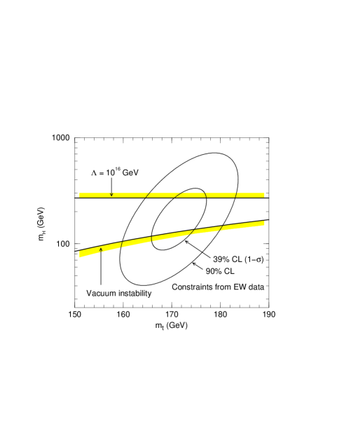
Figure 1: Constraint on the Higgs boson mass for the electroweak precision measurement and the theoretical bounds of the Higgs potential. The contours are obtained from the SM fit to all electroweak data with $m_{t}=175\pm 6$ GeV, $\alpha_{s}=0.118\pm 0.003$ and $1/\bar{\alpha}(m_{Z}^{2})=128.75\pm 0.09$. The inner and outer contours correspond to $\Delta\chi^{2}=1$ $(\sim 39\%{\rm CL})$, and $\Delta\chi^{2}=4.61$ $(\sim 90\%{\rm CL})$, respectively [10]. The upper and lower lines come from the triviality and vacuum stability bounds for the cut-off scale $\Lambda\sim 10^{16}$ GeV.

In summary, we consider the following range of the Higgs boson mass

$$137.1+21x_{t}+2.3x_{s}<m_{H}~{}({\rm GeV})<270,$$ (16)

in our analysis. We show in Fig. 1 the allowed region of the Higgs boson mass which is obtained from the SM fit to all electroweak precision measurements [10], where the contours are obtained from the SM fit to all the electroweak data and the external constraints $m_{t}=175\pm 6$ GeV [13], $\alpha_{s}=0.118\pm 0.003$ [12] and $1/\bar{\alpha}(m_{Z}^{2})=128.75\pm 0.09$ [8]. Theoretically allowed region of $m_{H}$, eq. (16), is also shown in the figure. It is clearly seen that the theoretically allowed range of $m_{H}$ with $\Lambda>10^{16}~{}{\rm GeV}$ is in perfect agreement with the constraint from these precision electroweak experiments.

The 2-loop RGE for the gauge couplings $\hat{\alpha}_{i}(\mu)$ in the $\overline{{\rm MS}}$ scheme is given as follows;

$$\mu\frac{d\hat{\alpha}_{i}}{d\mu}=\frac{1}{2\pi}b_{i}\hat{\alpha}_{i}^{2}+\frac{1}{8\pi^{2}}\hat{\alpha}_{i}^{2}\biggl{[}b_{ij}\hat{\alpha}_{j}+c_{ik}\frac{\hat{y}_{k}^{2}}{4\pi}\biggr{]},$$ (17)

where $i=1,2,3$ and $k=t,b,\tau$. The U(1) hyper-charge normalization is taken as $\hat{\alpha}_{1}=k_{Y}\hat{\alpha}_{Y}$. The term $\hat{y}_{k}$ denotes the $\overline{{\rm MS}}$ Yukawa coupling. The coefficients $b_{i},b_{ij}$ and $c_{ik}$ are given in the minimal SM as [17];

$$b_{i} = \biggl{(}\displaystyle{\frac{1}{k_{Y}}\frac{41}{6},-\frac{19}{6},-7\biggr{)}},$$ (18a)

$$b_{ij} = \left(\begin{array}[]{ccc}\displaystyle{\frac{1}{k_{Y}^{2}}\frac{199}{18}}&\displaystyle{\frac{1}{k_{Y}}\frac{9}{2}}&\displaystyle{\frac{1}{k_{Y}}\frac{44}{3}}\\ \vskip 8.5359pt\cr\displaystyle{\frac{1}{k_{Y}}\frac{3}{2}}&\displaystyle{\frac{35}{6}}&12\\ \vskip 8.5359pt\cr\displaystyle{\frac{1}{k_{Y}}\frac{11}{6}}&\displaystyle{\frac{9}{2}}&-26\end{array}\right),$$ (18e)

$$c_{ik} = \left(\begin{array}[]{ccc}\displaystyle{-\frac{1}{k_{Y}}\frac{17}{6}}&\displaystyle{-\frac{1}{k_{Y}}\frac{5}{6}}&\displaystyle{-\frac{1}{k_{Y}}\frac{5}{2}}\\ \vskip 8.5359pt\cr\displaystyle{-\frac{3}{2}}&\displaystyle{-\frac{3}{2}}&\displaystyle{-\frac{1}{2}}\\ \vskip 8.5359pt\cr-2&-2&0\end{array}\right).$$ (18i)

The $\overline{{\rm MS}}$ Yukawa coupling for fermion $f$ is given in terms of the corresponding pole mass $m_{f}$ as

$$\hat{y}_{f}(\mu)=2^{3/4}G_{F}^{1/2}m_{f}\{1+\delta_{f}(\mu)\},$$ (19)

where the factor $\delta_{f}(\mu)$ denotes the QCD and electroweak corrections. Because only the top-quark Yukawa coupling is found to affect our results significantly, we set $\hat{y}_{b}=\hat{y}_{\tau}=0$. The explicit form of $\delta_{t}(\mu)$ has been given in ref. [18]. Only the leading order $\mu$-dependence of $\hat{y}_{t}(\mu)$ is needed in our analysis [17];

$$\mu\frac{d}{d\mu}\biggl{(}\frac{\hat{y}_{t}^{2}}{4\pi}\biggr{)} = \frac{1}{2\pi}\biggl{(}\frac{\hat{y}_{t}^{2}}{4\pi}\biggr{)}\left[-\frac{1}{k_{Y}}\frac{17}{12}\hat{\alpha}_{1}-\frac{9}{4}\hat{\alpha}_{2}-8\hat{\alpha}_{3}+\frac{9}{2}\biggl{(}\frac{\hat{y}_{t}^{2}}{4\pi}\biggr{)}\right].$$ (20)

We can now solve the RGE in the NLO level and find the unification scale $m_{U}$ and the unified coupling $\alpha_{U}$ as functions of $\alpha_{s}(m_{Z})$, $m_{t},m_{H}$ and $\bar{\alpha}(m_{Z}^{2})$.

We show the result of our numerical study in Fig. 2. In order to show the $\alpha_{s}(m_{Z})$-dependence explicitly, we choose $m_{t}=175~{}{\rm GeV},m_{H}=100~{}{\rm GeV}$ and $1/\bar{\alpha}(m_{Z}^{2})=128.75$ in Fig. 2a. In the other figures, we fixed $\alpha_{s}(m_{Z})=0.118$ in Figs. 2b, 2c and 2d, $m_{t}=175~{}{\rm GeV}$ in Figs. 2c and 2d, $m_{H}=100~{}{\rm GeV}$ in Figs. 2b and 2d, and $1/\bar{\alpha}(m_{Z}^{2})=128.75$ in Figs. 2b and 2c.

Figure 2: Four parameter dependences of the SU(2)_L and SU(3)_C running couplings. Each figures correspond to: a) $\alpha_{s}(m_{Z})=0.118\pm 0.003$, b) $160~{}{\rm GeV}<m_{t}<190~{}{\rm GeV}$, c) $100~{}{\rm GeV}<m_{H}<270~{}{\rm GeV}$, d) $1/\bar{\alpha}(m_{Z}^{2})=128.75\pm 0.09.$

From Fig. 2, it is clearly seen that the 2-loop RGE gives the unification scale $m_{U}$ which is much smaller than the 1-loop RGE estimate of eq. (S0.EGx2). The scale $m_{U}$ increases for larger $\alpha_{s}(m_{Z})$, larger $\bar{\alpha}(m_{Z}^{2})$, larger $m_{H}$, and for smaller $m_{t}$. We find the following parametrization:

$$m_{U} = 2.75+0.93x_{s}+0.13x_{s}^{2}-0.20x_{t}+0.30x_{H}+0.03x_{H}^{2}$$ (21a)

$$~{}~{}~{}~{}~{}~{}~{}-0.04x_{\alpha}~{}~{}~{}~{}~{}(\times 10^{16}~{}{\rm GeV}),$$

$$\alpha_{U}^{-1} = 46.15+0.16x_{s}-0.07x_{t}+0.12x_{H}+0.004x_{H}^{2}-0.02x_{\alpha},$$ (21b)

for the unification scale $m_{U}$ and the unified coupling $\alpha_{U}$. It is remarkable that the unification scale of the minimal SM as determined above is almost the same as that of the MSSM, eq. (2). We can find from eq. (21a) that the largest value of the unification scale is $m_{U}\sim 4.4\times 10^{16}~{}{\rm GeV}$ for $\alpha_{s}(m_{Z})=0.121,m_{t}=165~{}{\rm GeV},m_{H}=270~{}{\rm GeV}$ and $1/\bar{\alpha}(m_{Z}^{2})=128.66$. Even with the extreme choice of $\alpha_{s}(m_{Z})=0.124~{}(x_{s}=2)$, the scale can reach $m_{U}\sim 5.7\times 10^{16}~{}{\rm GeV}$. It is still smaller than the expected string scale about one order of magnitude.

Figure 3: Parameter $\Delta$ as a function of the hyper-charge Kac-Moody level $k_{Y}$ for $m_{t}=175~{}{\rm GeV},m_{H}=100~{}{\rm GeV}$, and $1/\bar{\alpha}(m_{Z}^{2})=128.75$. The desired $k_{Y}$ is given at $\Delta=0$ where the three gauge couplings are unified.

The above result tells us that the string unification requires either extra matter particles or non-perturbative effects, as discussed in ref. [4], even in the non-SUSY minimal SM. There may also be a possibility that the 2-loop string effects can lower the unification scale. The desired Kac-Moody level $k_{Y}$ is then found by studying the difference

$${\Delta\equiv 1/\hat{\alpha}_{1}(m_{U})-1/\alpha_{U}},$$ (22)

where $\hat{\alpha}_{1}(\mu)=k_{Y}\hat{\alpha}_{Y}(\mu)$. In the absence of the significant string threshold corrections among the gauge couplings, the desired range of $k_{Y}$ that gives the unification of all three gauge couplings is determined by the condition $\Delta=0$. We show $\Delta$ as a function of $k_{Y}$ in Fig. 3 for $m_{t}=175~{}{\rm GeV}$, $m_{H}=100$ GeV and $1/\bar{\alpha}(m_{Z}^{2})=128.75$. We find that the unification is achieved when $1.33~{}{\mathop{<}\limits_{\sim}}~{}k_{Y}~{}{\mathop{<}\limits_{\sim}}~{}1.35$ for $\alpha_{s}(m_{Z})=0.118\pm 0.003$. On the other hand, the SU(5) case, $k_{Y}=5/3$, gives $\Delta=-9.02\pm 0.38$.

To summarize, we have quantitatively studied the possibility of the gauge coupling unification of the minimal non-SUSY SM at the string scale with a non-standard Kac-Moody level $k_{Y}$. Taking into account of the threshold corrections at the boundary of the RGE given by $m_{t}$ and $m_{H}$, and the uncertainties in $\alpha_{s}(m_{Z})$ and $\bar{\alpha}(m_{Z}^{2})$, we calculated the unification scale $m_{U}$ in the next-to-leading order. Current theoretical and experimental knowledge then tells us that the unification scale should satisfy $m_{U}~{}{\mathop{<}\limits_{\sim}}~{}4\times 10^{16}~{}{\rm GeV}$, which is one order of magnitude smaller than the naive string scale of $5\times 10^{17}~{}{\rm GeV}$ [2, 3]. If non-perturbative string effects or perturbative higher order effects can lower the string scale, then the hyper-charge Kac-Moody level should be $1.33~{}{\mathop{<}\limits_{\sim}}~{}k_{Y}~{}{\mathop{<}\limits_{\sim}}~{}1.35$.

We thank H. Aoki and H. Kawai for fruitful discussions. The work of G.C.C. is supported in part by Grant-in-Aid for Scientific Research from the Ministry of Education, Science and Culture of Japan.

References

• [1] D.J. Gross, J.A. Harvey, E. Martinec and R. Rohm, Nucl. Phys. B256 (1985) 253.
• [2] V. Kaplunovsky, Nucl. Phys. B307 (1988) 145, B382 (1992) 436 (E).
• [3] K.R. Dienes, Phys. Rept. 287 (1997) 447 (hep-th/9602045).
• [4] E. Witten, Nucl. Phys. B471 (1996) 135.
• [5] P. Ginsparg, Phys. Lett. B197 (1987) 139.
• [6] H. Aoki and H. Kawai, hep-ph/9703421, to be published in Prog. Theor. Phys.
• [7] K. Hagiwara, D. Haidt, C.S. Kim and S. Matsumoto, Z. Phys. C64 (1994) 559, C 68 (1995) 352 (E).
• [8] S. Eidelman and F. Jegerlehner, Z. Phys. C67 (1995) 585.
• [9] A.D. Martin and D. Zeppenfeld, Phys. Lett. B345 (1995) 558.
M.L. Swartz, Phys. Rev. D53 (1995) 5268.
H. Burkhardt and B. Pietrzyk, Phys. Lett. B356 (1995) 398.
• [10] K. Hagiwara, D. Haidt and S. Matsumoto, hep-ph/9706331, to be published in Z. Phys. C.
• [11] M.E. Peskin and T. Takeuchi, Phys. Rev. Lett. 65 (1990) 964, Phys. Rev. D46 (1992) 381.
• [12] Particle Data Group, R.M.Β Barnett et al., Phys. Rev. D54 (1996) 1.
• [13] CDF Collaboration, J.Β Lys, talk at ICHEP96, in Proc. of ICHEP96, (ed) Z. Ajduk and A.K. Wroblewski, World Scentific, (1997).
D0 Collaboration, S.Β Protopopescu, talk at ICHEP96, in the proceedings.
P.Β Tipton, talk at ICHEP96, in the proceedings.
• [14] G. Altarelli and G. Isidori, Phys. Lett. B337 (1994) 141.
• [15] J.A. Casas, J.R. Espinosa and M. Quiros, Phys. Lett. B342 (1995) 171.
• [16] J.S. Lee and J.K. Kim, Phys. Rev. D53 (1996) 6689.
• [17] C. Ford, D.R.T. Jones and P.W. Stephenson, Nucl. Phys. B395 (1993) 17.
• [18] R. Hempfling and B.A. Kniehl, Phys. Rev. D51 (1995) 1386.