Reheating in the Presence of Noise

Abstract

Explosive particle production due to parametric resonance is a crucial feature of reheating in inflationary cosmology. Coherent oscillations of the inflaton field act as a periodically varying mass in the evolution equation for matter fields which couple to the inflaton. This in turn results in the parametric resonance instability. Thermal and quantum noise will lead to a nonperiodic perturbation in the mass. We study the resulting equation for the evolution of matter fields and demonstrate that noise (at least if it is temporally uncorrelated) will increase the rate of particle production. We also estimate the limits on the magnitude of the noise for which the resonant behavior is qualitatively unchanged.

BROWN-HET-1072 August 1997.

hep-ph/yymmdd Typeset in REVTeX

I Introduction

Over the past few years, it has been realized that explosive particle production at the end of the period of inflation is a crucial aspect of inflationary cosmology. At the end of the period of exponential expansion, the energy density of matter and radiation is exponentially small, and without a very fast transfer of energy from the inflaton to ordinary matter, it is not possible to obtain a high post-inflationary temperature.

As was first pointed out in [1] and discussed in more detail in [2, 3, 4] and many other recent papers${}^{\cite[cite]{[\@@bibref{Number}{recent}{}{}]}}$, an oscillating scalar field induces a parametric resonance instability in the mode equations of any bosonic matter fields which couple to it. In particular, this applies to the inflaton, the scalar field responsible for inflation. At the end of the period of exponential expansion of the Universe, the inflaton is predicted to be performing homogeneous oscillations about its vacuum state. This will lead to instabilities in the mode equations of any bosonic matter field which couples to the inflaton, and this instability corresponds to explosive particle production.

Instabilities, due to resonance effects, are in general quite sensitive to the presence or absence of noise. In a real physical system we expect some non-periodic noise in the evolution of the inflaton. Such noise could be due to quantum fluctuations (the same quantum zero point oscillations which are believed to be the source of classical density perturbations${}^{\cite[cite]{[\@@bibref{Number}{flucts}{}{}]}}$ in the inflationary Universe scenario) or thermal fluctuations. In both cases, the amplitude of this noise is expected to be very small. Nevertheless, it is important to analyse the effects of this noise on parametric resonance.

In this paper, we study the effects of noise in the inflaton field on the evolution equation of matter fields which couple to the inflaton. As a first step, we take the noise to be homogeneous in space. In a subsequent paper we plan to study the (more realistic) case of inhomogeneous noise. Our main result is that noise which is not correlated temporally will on the average lead to an increase in the rate of particle production. We also derive limits on the amplitude of the noise for which the parametric resonance behavior persists. This result eliminates a further doubt on the effectiveness of resonance in realistic inflationary models. Most of our results apply for both narrow and broad-band resonance. For simplicity we neglect the expansion of the Universe; however, we do not believe that including effects of expansion would change our main conclusions.

In this paper we shall consider a simple model of reheating in the presence of a spatially homogeneous noise term. The inflaton field is taken to be a real scalar field and is denoted by $\varphi$. In the period immediately after inflation, $\varphi(t)$ is assumed to be oscillating coherently about (one of) its ground state(s). We shall, however, include a small aperiodic perturbation, i.e.

$$\varphi(t)=Acos(\omega t)+q(t)\,,$$ (1)

where $\omega$ is the natural frequency of oscillation of $\varphi$ and $q(t)$ denotes the noise.

We shall (following [1, 2, 3]) take $\varphi$ to be coupled to a second scalar field $\chi$ (which represents matter) via an interaction Lagrangian which is quadratic in $\chi$, for example of the form

$${\cal L}_{int}\propto{1\over 2}\varphi\chi^{2}\,.$$ (2)

To simplify the discussion, we neglect nonlinearities in the equation of motion for $\chi$. Such nonlinearities may very well be important and lead to an early termination of parametric resonance. This issue has recently been discussed extensively, see e.g. [7, 8, 9], but is not the topic of our paper. Instead, we are interested whether the presence of noise such as included in (1) will effect the onset of resonance.

For simplicity, we will neglect the expansion of the Universe. In [1, 2, 3] it has been shown that the expansion can be included without difficulty, and that it does not prevent the onset of the parametric resonance instability. Since the equation of motion for $\chi(x,t)$ is linear and translation invariant, the Fourier modes evolve independently. We can immediately write down the evolution equations for the Fourier modes of $\chi$, denoted by $\chi_{k}$, in the case of “coherent” noise. They take the form

$$\ddot{\chi_{k}}+\left[\omega_{k}^{2}+(p(\omega t)+q(t))\right]\chi_{k}=0\,,$$ (3)

where $p(x)$ is a periodic function whose frequency is $2\pi$, $q(t)$ represents the noise which we consider as a perturbation of the driving function $p(t)$, and

$$\omega_{k}^{2}=m_{\chi}^{2}+k^{2}\,.$$ (4)

Note that our analysis applies both to the case of narrow-band${}^{\cite[cite]{[\@@bibref{Number}{TB,stb}{}{}]}}$ ($p/{\omega^{2}}\ll 1$) and broad-band${}^{\cite[cite]{[\@@bibref{Number}{kls94}{}{}]}}$ ($p/{\omega^{2}}\gg 1$) resonance.

By assumption, $q(t)$ is a small perturbation of $\varphi(t)$. Hence, it is suppressed compared to $p(t)$, and in order to represent this, we write

$$q(t)=g\omega^{2}n(t)\,,$$ (5)

where $n(t)$ is a dimensionless “noise function” of amplitude 1, and where we have introduced the dimensionless small coupling $g$ by extracting the dimensions of $q$ by means of the factor $\omega^{2}$.

We wish to consider how the presence of noise in the inflaton effects the excitation of the matter field components $\chi_{k}$ from their vacuum state. Another way in which thermal noise can effect the calculation has recently been studied in [10] where it was shown that parametric resonance is also effective if we consider the field $\chi$ to be initially in a thermal state.

We can study this problem in three ways (see e.g. [11] for a recent review). First, we study the effects of the noise on the solutions of the classical equation of motion (3) using the method of successive approximations and the Furstenberg theorem on products of random matrices. Next, we use the Bogoliubov mode mixing technique ${}^{\cite[cite]{[\@@bibref{Number}{bogol}{}{}]}}$ to analyze the change in the solutions due to the noise. This method is closely related to a consistent semiclassical analysis which treats the excitation of the $\chi$ field as a problem of quantum field theory in a classical background inflaton field (see e.g. Appendix B of [3]). Finally, we study the effects of the noise using the Born approximation and compare with numerical results.

II Exact Results

The principal results of this section are that the exponential growth rate of solutions is a continuous quantity with respect to $q(t)$, so that a small addition of noise will not change it overly. Furthermore, under reasonable assumptions of decorrelation of the noise, the growth rate is shown to be always strictly increased by the noise. For these considerations it proves convenient to rephrase our basic second order differential equation (3) as a first order $2\times 2$ matrix differential equation

$${\dot{\Phi}_{q}}\,=\,M(q(t),t)\Phi_{q}$$ (6)

with initial conditions $\Phi_{q}(0,0)=I$. Here, $M(q(t),t)$ is the matrix

$$M(q(t),t)\,=\,\left(\begin{array}[]{cc}0&1\\ -(\omega_{k}^{2}+p(t)+q(t))&0\end{array}\right)\,,$$ (7)

and $\Phi_{q}(\tau,\sigma)$ is the fundamental solution (or transfer) matrix from time $\sigma$ to time $\tau$;

$$\Phi_{q}(t,0)\,=\,\left(\begin{array}[]{cc}\phi_{1}(t;q)&\phi_{2}(t;q)\\ {\dot{\phi}_{1}(t;q)}&{\dot{\phi}_{2}(t;q)}\end{array}\right)\,,$$ (8)

consisting of two independent solutions $\phi_{1}(t;q)$ and $\phi_{2}(t;q)$ of the second order equation (3).

For vanishing noise, i.e. $q(t)=0$, the content of Floquet theory is that the solution of (6) can be written in the form

$$\Phi_{0}(t,0)\,=\,P_{0}(t)e^{Ct}\,,$$ (9)

where $P_{0}(t)$ is a periodic matrix function with period $T=1/\omega$, and $C$ is a constant matrix whose spectrum in a resonance region is $spec(C)=\{\pm\mu(0)\}$.

We would like the noise $q(t)$ to correspond to random quantum or thermal fluctuations superimposed on the periodic classical oscillation of the inflaton field $\varphi(t)$. Our picture is that of fluctuations driven by Brownian motion, however for the purposes of deriving the exact results to be presented here, it is sufficient to make certain statistical assumptions about the noise $q(t)$. These are phrased in terms of a sample space $\Omega$ from which the realizations $\kappa$ of the noise $q(t)=q(t;\kappa)$ are drawn. On the sample space $\Omega$ there is a probability measure $dP(\kappa)$, and expectation values of functions $f(\kappa)$ with respect to this measure are denoted by

$\displaystyle E(f)\,=\int dP(\kappa)f(\kappa)\,.$For our purposes we may take $\Omega=C({\mathbf{R}})$, the space of bounded continuous functions on ${\mathbf{R}}$, and $dP(\kappa)$ on $\Omega$ a translation invariant measure. We assume that the noise is ergodic, which is to say that

$$E(f(q))\,=\,\lim_{t\rightarrow\infty}{1\over t}\int_{0}^{t}d\tau\ f(q(\cdot+\tau;\kappa_{0}))$$ (10)

for almost all $dP(\kappa)$ realizations $\kappa_{0}$ of the noise.

The first relevant mathematical result (Proposition 1, see Appendix) is that the growth rate (the generalized Floquet exponent, or Lyapunov exponent) of the solutions of (6) is well defined by the limit

$$\mu(q)\,=\,\lim_{N\rightarrow\infty}{1\over{NT}}\log\|\Pi_{j=1}^{N}\Phi(jT,(j-1)T)\|\,,$$ (11)

where $\|\cdot\|$ denotes some matrix norm (the dependence on the specific norm drops out in the large $N$ limit). The limit in (11) exists for almost every sample (with respect to $dP(\kappa)$), and it is almost everywhere $dP(\kappa)$ constant, which is to say that it depends only upon the the statistics of samples $q(t;\kappa)$ and not on the individual realizations.

The first qualitative result (Proposition 2, see Appendix) is that the growth rate $\mu(q)$ is continuous in $q$ in an appropriate topology on $\Omega$ (the topology on $C({\mathbf{R}})$ of uniform convergence on compact sets). In particular, this implies that if we write the noise as in (5) in terms of a dimensionless strength $g$ and view the statistics of the noise as a measure on the function space of $n(t)$, then $\mu(q)$ converges to $\mu(0)$ as $g$ converges to zero. We remark that Propositions 1 and 2 do not depend on the fact that the system is one-dimensional, and will thus also hold for inhomogeneous noise.

The limit (11) also describes $\mu(0)$, which is implicitly a function of the background periodic potential $p(t)$; it shows in particular that $\mu(0)\geq 0$. A second qualitative estimate (Theorem 3, see Appendix and [18]) is that, if the support of the probability measure $dP(\kappa)$ on the space $C({\mathbf{R}})$ includes the sample $q(t)=0$, then $\mu(q)>0$ whenever $\mu(0)>0$.

The results cited above do not give insight into the quantitative value of the growth rate in the presence of noise. A first step in this direction is given by the following theorem. Suppose that the statistics of the noise are such that

  

(i) The noise $q(t)$ is uncorrelated in time on scales larger than $T$, that is, $\{q(t;\kappa)\,:\,jT\leq t\leq(j+1)T\}$ is independent of $\{q(t;\kappa)\,:\,lT\leq t\leq(l+1)T\}$ for integers $l\neq j$, and is identically distributed.

  

(ii) Restricting the noise $q(t;\kappa)$ to the time interval $0\leq t<T$, the samples $\{q(t;\kappa):0\leq t<T\}$ within the support of the probability measure fill a neighborhood, in $C(0,T)$, of the origin.

Hypothesis (i) implies that the noise is ergodic, and therefore the generalized Floquet exponent is well defined. We will show (Theorem 4, Appendix) that in fact $\mu(q)$ is strictly larger than $\mu(0)$;

$$\mu(q)\,>\,\mu(0)\,,$$ (12)

which demonstrates that the presence of noise leads to a strict increase in the rate of particle production. This is a quantitative lower bound on the generalized Floquet exponent with noise. Our result is based on an application of Furstenberg’s theorem, concerning the Lyapunov exponent of products of independent identically distributed random matrices $\{\Psi_{j}:j=1,...,N\}$. It states that (modulo certain assumptions which are shown to hold in the Appendix)

$$\lim_{N\rightarrow\infty}{1\over{NT}}\log\|\Pi_{j=1}^{N}\Psi_{j}\|\,=\,\lambda\,>\,0\,,$$ (13)

where $\lambda=\lambda(q)$ depends again only on the statistics of $\Psi_{j}$, and not on the individual samples. A further result is that for any nonzero vectors $v_{1}$ and $v_{2}$ and for almost all $\{\Psi_{j}(\kappa)\}_{j=1}^{\infty}$

$$\lim_{N\rightarrow\infty}{1\over{NT}}\log\langle v_{1},\Pi_{j=1}^{N}\Psi_{j}v_{2}\rangle\,=\,\lambda\,.$$ (14)

In order to apply Furstenberg’s theorem to obtain (12), we start by factoring out from the transfer matrix $\Phi_{q}(t,0)$ the contribution due to the evolution without noise;

$$\Phi_{q}(t,0)\,=\,\Phi_{0}(t,0)\Psi_{q}(t,0)\,=\,P_{0}(t)e^{Ct}\Psi_{q}(t,0)\,.$$ (15)

The reduced transfer matrix $\Psi_{q}(t,0)$ satisfies the following equation

$${\dot{\Psi}_{q}}\,=\,S(t;\kappa)\Psi_{q}\,=\,\Phi_{0}^{-1}(t)\left(\begin{array}[]{cc}0&0\\ -q(t;\kappa)&0\end{array}\right)\Phi_{0}(t)\Psi_{q}\,,$$ (16)

which can be written as a matrix integral equation

$$\Psi_{q}(t,0)\,=\,I+\int_{0}^{t}d\tau\ S(\tau;\kappa)\Psi_{q}(\tau,0)\,.$$ (17)

Solutions $\Psi_{q}(t,0)$ to (17) are constructed in the next section, using the method of successive approximation, giving rise to the transfer matrices $\Psi_{q}(jT,(j-1)T)$ which are the fundamental solution matrices for the period intervals of the background potential. By properties (ii) of decorrelation of the noise, the quantities $\Psi_{q}(jT,(j-1)T)$ are independent and identically distributed for different integers $j$, and we can apply the Furstenberg theorem to the following decomposition of $\Psi_{q}(NT,0)$;

$\displaystyle\Psi_{q}(NT,0)\,=\,\Pi_{j=1}^{N}\Psi_{q}(jT,(j-1)T)\,.$We may choose for instance the vector $v_{1}$ in (14) to be an eigenvector of $\Phi_{0}(T,0)^{t}=(P_{0}(T)e^{CT})^{t}$, the transpose of the transfer matrix of the system without noise, with eigenvalue $e^{\mu(0)T}$. Then (14) becomes

$${1\over{NT}}\log|\langle v_{1},\Phi_{q}(NT,0)v_{2}\rangle| = {1\over{NT}}\log|\langle v_{1},P_{0}(NT)e^{CNT}\Psi_{q}(NT,0)v_{2}\rangle|$$ (18)

$$= {1\over{NT}}\log(e^{\mu(0)NT}|\langle v_{1},\Psi_{q}(NT,0)v_{2}\rangle|)$$ (19)

$$= \mu(0)\,+\,{1\over{NT}}\log|\langle v_{1},\Pi_{j=1}^{N}\Psi_{q}(jT,(j-1)T)v_{2}\rangle|\,.$$ (20)

Taking the limit $N\rightarrow\infty$ and applying (13) and (14) we obtain

$$\mu(q)\,=\,\mu(0)+\lambda\,>\,\mu(0)$$ (21)

which proves the main result (12). Note in particular that (12) implies that even for modes which without noise are in a stability band ($\mu(0)=0$) there will be exponential particle production in the presence of noise. The fact that there is particle production due to the presence of noise is a nontrivial result, and the fact that the rate of particle production is exponential may be understood physically as a sign of stimulated emission. Note that, strictly speaking, the ergodic hypothesis is only satisfied in the $t\rightarrow\infty$ limit. Finite time intervals, such as the characteristic time of reheating $\mu^{-1}$, may be insufficient for the decorrelation of the noise. In this case, we may observe transient effects (see Section VII).

So far, our results have not given any quantitative upper bound for the growth rate of modes of $\chi$ in the presence of noise. Additionally, they do not show how the evolution of an individual solution is modified, as compared to what occurs in the system without noise. In the following sections we will give estimates on the magnitude of noise for which we can demonstrate that the parametric resonance behavior remains qualitatively unchanged. These estimates are then used in the proof in the appendix of the main result (12).

III An Estimate Using Successive Approximations

In this section we sketch the construction of the fundamental solution matrix $\Psi_{q}(t,0)$ for system (16), showing in particular that $\{\Psi_{q}(jT,(j-1)T)\}_{j=1}^{\infty}$ represents a sequence of independent identically distributed random matrices. The starting point for this estimate is the integral equation (17) for the reduced transfer matrix $\Psi(t,0)$ (dropping the subscript $q$ for notational ease). We solve this equation by constructing a sequence of approximate solutions

$$\Psi_{n+1}(t,0)\,=\,I\,+\,\int_{0}^{t}d\tau\ S(\tau;q(\tau))\Psi_{n}(\tau,0)$$ (22)

with $\Psi_{0}=I$. The differences between successive terms of the sequence satisfy

$$\Psi_{n+1}(t,0)-\Psi_{n}(t,0)\,=\,\int_{0}^{t}d\tau\ S(\tau;q(\tau))\bigl{(}\Psi_{n}(\tau,0)-\Psi_{n-1}(\tau,0)\bigr{)}\,.$$ (23)

We will apply this equation for evolution over the time period $T$.

By induction is can easily be shown that the successive differences satisfy the estimate

$$\|\Psi_{n+1}(T,0)-\Psi_{n}(T,0)\|\,\leq\,M^{n+1}{{T^{n+1}}\over{(n+1)!}}\,,$$ (24)

where the constant $M$ is

$$M\,=\,\sup_{0\leq s\leq T}\|S(s;q)\|\,.$$ (25)

From the definition of the matrix $S$ (see (16) and (9)) it follows that (if the norm $\|\cdot\|$ is taken to be the supremum norm or the norm mentioned after (11))

$$M\,\leq\,e^{2\mu(0)T}\|q(\cdot;\kappa)\|\,.$$ (26)

The following telescoping sum then describes the fundamental solution matrix;

$$\Psi(t,0)\,=\,\sum_{n=1}^{\infty}\bigl{(}\Psi_{n}(t,0)-\Psi_{n-1}(t,0)\bigr{)}+I~{},$$ (27)

and by using (24) we estimate that

$$\|\Psi(t,0)-I\| \,\leq\, \sum_{n=1}^{\infty}{(Mt)^{n}\over n\!}$$ (28)

$$\,=\, e^{Mt}-1\,\leq\,(Mt)e^{Mt}~{}.$$ (29)

The fundamental solution of (6) is $\Phi_{q}(t,0)=\Phi_{0}(t,0)\Psi_{q}(t,0)$, therefore the deviation between the solution with noise and the solution without it can be measured by the estimate

$$\|\Phi_{q}(t,0)-\Phi_{0}(t,0)\| \,=\, \|\Phi_{0}(t,0)(\Psi_{q}(t,0)-I)\|$$ (30)

$$\,\leq\, \|\Phi_{0}(t,0)\|\|R_{q}(t,0)\|~{},$$ (31)

where $R_{q}(t,0)=(\Psi_{q}(t,0)-I)$. When we set $q(t;\kappa)=g\omega^{2}n(t;\kappa)$, and $g$ is taken to zero, then the constant $M$ in (25) also converges to zero, therefore for fixed time $t$ the error $\|R_{q}(t,0)\|\leq(Mt)\exp(Mt)$ is small and thus solutions of the two equations which have the same initial data are shown to be close.

We will now make use of the above estimate in order to bound from above the difference $\mu(q)-\mu(0)$. We consider evolution over a time interval $NT$ and break up the transfer matrix into matrices corresponding to single periods $T$. From (15) and (11) we obtain

$$\mu(q)-\mu(0)\,=\,\lim_{N\rightarrow\infty}{1\over{NT}}E\bigl{(}\log\bigl{[}{{\|\Pi_{j=1}^{N}(P_{0}(T)e^{TC}\Psi_{q}(jT,(j-1)T))\|}\over{\|\Pi_{j=1}^{N}e^{TC}\|}}\bigr{]}\bigr{)}\,.$$ (32)

Making use of the periodicity of $P_{0}$, we can write the norm of the product in the numerator (denoted by $NUM$) as

$\displaystyle NUM\,=\,\|\Pi_{j=1}^{N}\bigl{(}e^{TC}+\Delta_{q}(jT,(j-1)T)\bigr{)}\|\,,$where $\Delta_{q}$ represents the difference in between the transfer matrices with and without noise. We need to bound its contribution in magnitude from above. Due to the fact that the noise is uncorrelated over time intervals larger than $T$, this needs to be done only for one period. Introducing the symbol

$$\Theta\,=\,E\bigl{(}{{\|\Delta_{q}(T,0)\|}\over{\|e^{TC}\|}}\bigr{)}\,,$$ (33)

we can bound the difference in the generalized Floquet exponents (32) by

$$\mu(q)-\mu(0)\,\leq\,\lim_{N\rightarrow\infty}{1\over{NT}}\log(1+\Theta)^{N}\,=\,{1\over T}\log(1+\Theta)\,,$$ (34)

which for low amplitude noise can be approximated by $\Theta/T$.

Making use of the fact that $\mu(0)/\omega\ll 1$, it follows that for noise of the form given by (5), $\Theta$ is of the order $g\omega^{2}T^{2}$. Hence, from (34) we conclude that if

$$g\,\ll\,{{\mu(0)}\over{\omega}}$$ (35)

the effects of the noise do not significantly effect parametric resonance. Furthermore, the estimate (24) shows that solutions of (6) cannot deviate by more than $MT\exp(MT)$ from $\Phi_{0}(t,0)$, over time intervals of length $T$.

IV A Second Estimate Using Successive Approximations

The growth rate $\mu(q)$ of the previous section is the result of a limiting process over many periods $T$ of the background periodic excitation $p(t)$. It may be, however, that the noise acts over small characteristic subintervals of length $\Delta t$, and the reheating epoch only encompasses a finite and relatively small number of periods of the background. By studying directly the second order differential equation (3) with an estimate based on the method of successive approximations, we will exhibit in such a situation a bound in terms of the coupling constant $g$ on the deviation of solutions perturbed by the presence of noise from the unperturbed solution. In case this deviation is small when compared with the size of the unperturbed solution, we can conclude that the growth due to parametric resonance is not destroyed by the presence of the noise term. We obtain an estimate on $g$ for which this holds; it turns out to be of the same character as estimate (35).

The method is to rewrite equation (3) as an integral equation and to determine the general solution in terms of a series of successive approximations. In the following we use a well-known result for differential equations. Let $\chi(t)$ be the solution of the differential equation (we drop the index $k$ on $\chi$ to simplify the notation)

$$\ddot{\chi}+\left[\omega_{k}^{2}+(p(t)+q(t))\right]\chi=0\,,$$ (36)

subject to given initial conditions, and let $\chi_{h}$ be the solution of the unperturbed equation

$$\ddot{\chi}+\left[\omega_{k}^{2}+p(t)\right]\chi=0\,,$$ (37)

satisfying the same initial conditions. Then, Eq. (36) can be rewritten as an inhomogeneous Volterra equation${}^{\cite[cite]{[\@@bibref{Number}{Volterra}{}{}]}}$ of the second kind

$$\chi(t)=\chi_{h}(t)+\int_{t_{i}}^{t}\left[{\phi_{1}(t^{{}^{\prime}})\phi_{2}(t)-\phi_{1}(t)\phi_{2}(t^{{}^{\prime}})\over W}\right]\left[-q(t^{{}^{\prime}})\chi(t^{{}^{\prime}})\right]dt^{{}^{\prime}}\,,$$ (38)

where $\phi_{1}$ and $\phi_{2}$ are two independent solutions of equation (37) and $W$ is their Wronskian, which is independent of time (by Abell’s formula, see e.g. [15]). We then apply the method of successive approximations starting with the unperturbed solution $\chi_{h}(t)$. We define recursively

$$\chi_{0}(t) = \chi_{h}(t)\,,$$ (39)

$$\chi_{n}(t) = \chi_{h}(t)+\int_{t_{i}}^{t}\left[{\phi_{1}(t^{{}^{\prime}})\phi_{2}(t)-\phi_{1}(t)\phi_{2}(t^{{}^{\prime}})\over W}\right]\left[-q(t^{{}^{\prime}})\chi_{n-1}(t^{{}^{\prime}})\right]dt^{{}^{\prime}}\,\quad n\geq 1\,.$$ (40)

From the above, we get an appropriate estimate for the successive approximations

$$\chi_{n+1}(t)-\chi_{n}(t)=\int_{t_{i}}^{t}\left[{\phi_{1}(t^{{}^{\prime}})\phi_{2}(t)-\phi_{1}(t)\phi_{2}(t^{{}^{\prime}})\over W}\right]\left[-q(t^{{}^{\prime}})\right]\left[\chi_{n}(t^{{}^{\prime}})-\chi_{n-1}(t^{{}^{\prime}})\right]dt^{{}^{\prime}}\,.$$ (41)

The function $p(t)$ is periodic, so that the two independent solutions of equation (37) can be written in Floquet’s form${}^{\cite[cite]{[\@@bibref{Number}{Floquet}{}{}]}}$

$$\phi_{1}(t)=e^{\mu(0)t}p_{1}(t)\,,\hskip 28.45274pt\phi_{2}(t)=e^{-\mu(0)t}p_{2}(t)\,,$$ (42)

where $p_{1}$ and $p_{2}$ are both periodic functions of time with period $T$, and $\mu(0)$ is the Floquet exponent discussed in the previous section. Let us focus on the behavior of the solution over an arbitrary time interval $I=[t_{i},t_{f}]$, of length $\Delta T$. Define

$$M_{1}=\max_{0\leq t\leq T}|p_{1}(t)|\,,\quad M_{2}=\max_{0\leq t\leq T}|p_{2}(t)|\,.\\$$ (43)

According to our assumptions, the perturbation $q(t)$ is bounded by $g\omega^{2}$,

$$\max_{t\in{\bf R}}\left|q(t)\right|\leq g\omega^{2}<+\infty\,.$$ (44)

Defining the norm

$$\|\chi_{n}-\chi_{n-1}\|=\max_{t\in I}|\chi_{n}(t)-\chi_{n-1}(t)|\,,$$ (45)

and using equations (41)–(44) it follows that for $t\in I$ then

$$|\chi_{n+1}(t)-\chi_{n}(t)|\leq\,\Bigl{(}2g\omega^{2}{{M_{1}M_{2}}\over{|W|}}e^{\mu(0)\Delta T}\Bigr{)}^{n+1}{(t-t_{i})^{n+1}\over(n+1)!}\|\chi_{h}\|\,.$$ (46)

Define

$$\alpha=2g\omega^{2}{M_{1}M_{2}\over|W|}e^{\mu(0)\Delta T}\,.$$ (47)

Let us now estimate the distance $d=\|\chi-\chi_{h}\|$. We consider the telescopic series

$$\chi_{n+1}(t)-\chi_{h}(t)=\sum_{j=0}^{n}(\chi_{j+1}-\chi_{j})\,,$$ (48)

and use equations (46) and (47) and the triangle inequality to obtain

$$|\chi_{n+1}(t)-\chi_{h}(t)|\,\leq\,\sum_{j=0}^{n}|\chi_{j+1}(t)-\chi_{j}(t)|\,\leq\,\sum_{j=0}^{n}\alpha^{j+1}{(t-t_{i})^{j+1}\over(j+1)!}\|\chi_{h}\|\,,$$ (49)

where $\alpha$ is given by (47). Taking the limit $n\to\infty$ and using the definition of the norm in (45) we obtain

$$\|\chi-\chi_{h}\|\,\leq\,(e^{\alpha\Delta T}-1)\|\chi_{h}\|\,\leq\,\alpha\Delta Te^{\alpha\Delta T}\|\chi_{h}\|\,.$$ (50)

The last step is to ensure that the unperturbed solution has undergone appreciable growth by the end of the considered time interval. Typical initial data for the problem is of the form

$$\chi_{h}(t)\,=\,c_{1}\phi_{1}(t)\,+\,c_{2}\phi_{2}(t)\,,$$ (51)

with coefficients $c_{1}$ and $c_{2}$ which are of the order 1, therefore $\|\chi_{h}\|=O(\exp(\mu(0)\Delta T))$.

Note that the period of reheating in the absence of the noise is $N\mu(0)^{-1}$, with $N$ being a number of the order $2\times{\rm log}(\eta/H)$ (where $H$ is the expansion rate of the Universe and $\eta$ is the energy scale of inflation). A typical value of $\eta/H$ is of the order $10^{6}$, and this implies that the number $N$ is not necessarily large. Hence, for practical purposes it is sufficient to control the effects of the noise over a time interval $\mu(0)^{-1}$. In addition, in order to prove that the effects of the noise are small compared to the unperturbed solution, we must consider time intervals over which the unperturbed solution has significant exponential growth, i.e. over which the growing mode solution of equation (37), $\phi_{1}(t)$, dominates the decaying mode $\phi_{2}(t)$. This provides another reason to consider time intervals such that $\mu(0)\Delta T>1$. To be definite we will take $\mu(0)\Delta T=2$.

The maximal distance $d$ between $\chi$ and $\chi_{h}$ is controlled by (50) over any interval $I$. If the amplitude of the noise is sufficiently small, then this distance will not be appreciable when compared with the size of $\chi_{h}$. In order for this to be true, we require that

$$\alpha\Delta Te^{\alpha\Delta T}\leq{1\over 2}\,.$$ (52)

The condition of smallness which emerges from (52) is that

$$\alpha\Delta T=2e^{2}g\omega^{2}(M_{1}M_{2}/|W|)\Delta T<<1\,.$$ (53)

To obtain an estimate of the order of magnitude of this constraint, we note that $|W|\,\sim\,M_{1}M_{2}\omega$. Inserting this into (53) we obtain

$$g\,\ll\,{\mu(0)\over{\omega}}\,,$$ (54)

which is the same requirement as was obtained in the previous section (35). Thus, in this case the parametric resonance growth of $\chi_{h}(t)$ is preserved in $\chi(t)$.

Certainly there are better estimates that can be obtained if more information about the noise is provided. On the other hand, we have shown that for any kind of small homogeneous noise, over time intervals of length $\Delta T=O(\mu(0)^{-1})$, parametric resonance is not destroyed by the presence of low amplitude noise in the inflaton field.

V An Analysis via the Bogoliubov Method

Another approach which can be used to demonstrate that random noise with a small amplitude does not eliminate the parametric resonance instability is the Bogoliubov method${}^{\cite[cite]{[\@@bibref{Number}{bogol}{}{}]}}$. This approach has the advantage of giving some information on how the noise effects the dynamics. However, it is less rigorous than the method of successive approximations and holds only in the case of narrow resonance regime.

The evolution equation for $\chi_{k}(t)$ in the presence of the oscillating inflaton field (see Eq. (3)) is (dropping the subscript $k$ and introducing an explicit expansion parameter $\varepsilon\ll 1$)

$$\ddot{\chi}(t)+\left[\omega_{k}^{2}+\varepsilon\Bigl{(}p(\omega t)+q(t)\Bigr{)}\right]\chi(t)=0\,,$$ (55)

where $p(\omega t)$ is a function with period $2\pi/\omega$ and $q(t)$ represents the noise.

For simplicity we consider a mode $k$ which (in the absence of noise) is in the first resonance band, i.e. for which $2\omega_{k}=\omega-\Delta$, where $\Delta$ is a small quantity. In this case we may write:

$$p(\omega t)=\omega_{k}^{2}\,\cos(2\omega_{k}+\Delta)t\,,$$ (56)

with $-\varepsilon\omega_{k}<2\Delta<\varepsilon\omega_{k}$. Following the Bogoliubov method [12] we assume that, to first order in $\varepsilon$, the solution of (55) is of the form

$$\chi(t)=a(t)\cos(\omega_{k}+{\Delta\over 2})t+b(t)\sin(\omega_{k}+{\Delta\over 2})t\,,$$ (57)

where $a(t)$ and $b(t)$ vary slowly in comparison with the trigonometric factors. Notice that the exact solution includes terms with frequencies higher than $\omega_{k}+\Delta/2$. These terms are neglected in the first order solution since they are of higher order in $\varepsilon$.

Inserting (57) and (56) in (55) and keeping only first order terms we obtain

$$\left(\ddot{a}+\omega\dot{b}-{\Delta\over 2}\omega a+{\varepsilon\over 2}\omega_{k}^{2}a+\varepsilon qa\right)\cos(\omega_{k}+{\Delta\over 2})t$$ (58)

$$+\left(\ddot{b}-\omega\dot{a}-{\Delta\over 2}\omega b-{\varepsilon\over 2}\omega_{k}^{2}b+\varepsilon qb\right)\sin(\omega_{k}+{\Delta\over 2})t=0\,.$$ (59)

It is clear that the coefficients of both the cosine and sine in the above equation must be zero, which yields two differential equations for the functions $a(t)$ and $b(t)$. We seek solutions of the form

$$a(t)=A(t)e^{\mu t}\,,\quad\quad b(t)=B(t)e^{\mu t}\,,$$ (60)

where $\mu$ is a constant of order $\varepsilon$. We then get

$$\ddot{A}+2\mu\dot{A}+\omega\dot{B}+\mu\omega B-{\Delta\over 2}\omega A+{\varepsilon\over 2}\omega_{k}^{2}A+\varepsilon qA =0\,,$$ (61)

$$\ddot{B}+2\mu\dot{B}-\omega\dot{A}-\omega\mu A-{\Delta\over 2}\omega B-{\varepsilon\over 2}\omega_{k}^{2}B+\varepsilon{q}B =0\,.$$ (62)

Let us initially study the case when the noise is neglected. Since $q=0$, by following the Bogoliubov method we can assume that $\dot{A}$, $\dot{B}$, $\ddot{A}$ and $\ddot{B}$ are of second order in $\varepsilon$. The resulting system is (recalling that $\omega=2\omega_{k}+\Delta$)

$$2\mu A+B\Delta+{\varepsilon\over 2}\omega_{k}B=0\,,\quad 2\mu B-A\Delta+{\varepsilon\over 2}\omega_{k}A=0\,,$$ (63)

which yields

$$\mu^{2}={\omega_{k}^{2}\over 4}\left({\varepsilon^{2}\over 4}-{\Delta^{2}\over\omega_{k}^{2}}\right)\,,\quad\quad A\sim B=const.$$ (64)

This result means that as long as $\mu$ is real ($-\varepsilon\omega_{k}<{2\Delta}<\varepsilon\omega_{k}$) and for $q=0$ the $\chi_{k}$ field grows exponentially in time.

From the above analysis a simple but very important result follows. In the narrow resonance regime, the resonance is not destroyed by noise which is small compared to the amplitude of the oscillatory inflaton field $p(\omega t)$. Specifically, if $g$ (see (5)) is small, say $g=\it{O}(\varepsilon)$, then the last term in both of the equations (62) can be neglected and the result of Eqs. (64) follows.

On the other hand, when $q$ is not negligible, then the derivatives $\dot{A}$, $\dot{B}$, $\ddot{A}$ and $\ddot{B}$ must be of first order in $\varepsilon$ and not $O(\varepsilon^{2})$ as we assumed above. This can be seen as follows. Solving equations (62) as before under the assumption that the derivatives are negligible leads to a solution for $A$ and $B$ which depends on time (via the noise $q$), and whose derivatives are thus proportional to $\varepsilon\Gamma$, where $\Gamma$ is the rate of change of the noise. This demonstrates that the derivatives are not negligible.

In order to circumvent this difficulty we differentiate once equations (62) and neglect all terms of second and higher order in $\varepsilon$ to get the following

$$A^{{}^{{}^{\hskip-6.82881pt\mbox{...}}}}+\omega\ddot{B}+\varepsilon\dot{q}A =0\,,$$ (65)

$$B^{{}^{{}^{\hskip-7.68236pt\mbox{...}}}}-\omega\ddot{A}+\varepsilon\dot{q}B =0\,.$$ (66)

By integrating the above system we get (to first order in $\varepsilon$)

$$\ddot{A}+\omega\dot{B}+\varepsilon qA =C_{1}\,,$$ (67)

$$\ddot{B}-\omega\dot{A}+\varepsilon qB =C_{2}\,,$$ (68)

where $C_{1}$ and $C_{2}$ are both constants of order of $\varepsilon$.

The next step is to check the compatibility between (68) and (62). Inserting (68) into (62) and neglecting terms of order $\varepsilon^{2}$, we obtain a matrix equation for the vector $(A,B)$ which has a solution only if the determinant of the coefficient matrix vanishes. This condition leads to the same value of the Floquet exponent $\mu$ as obtained in the absence of noise (cf. Eq. (64)). Since $q(t)$ is a general time dependent function, a solution exists only if $C_{1}=C_{2}=0$, and only if the terms $\omega\dot{B}$ and $\omega\dot{A}$ in (68) are negligible compared to the other terms. Any other choice for $C_{1}$ and $C_{2}$ implies $A=const.$, $B=const.$, which is only the case for $g=O(\varepsilon)$ as we showed above.

Moreover, using (66) and (68) it is seen that conditions $|\omega\ddot{B}|\ll|\varepsilon{\dot{q}}A|$ and $|\omega\ddot{A}|\ll|\varepsilon{\dot{q}}B|$ are equivalent to $\omega\ll{|\dot{q}|}/{|q|}\sim\Gamma$, where $\Gamma$ is the characteristic rate of the noise. In this situation, Equations (68) reduce to $\ddot{A}+\varepsilon qA=0\,$, $\ddot{B}+\varepsilon qB=0\,$, whose solutions to first order in $\varepsilon$ can be written as $A\,,B\propto e^{-\gamma(t)}$, where $\gamma(t)=\varepsilon\int_{o}^{t}\Psi(\tau)d\tau$ with $\dot{\Psi}=q\equiv g\omega^{2}n(t)$ (see Eq. (5)).

In this case, parametric resonance can be destroyed by possible exponential decay of $A$ and $B$. For assume that $t$ is sufficiently big and that the noise $n(t)$ is a random walk, so that we can define the average of $n$ in the time interval from $0$ to $t$ as $\bar{n}={1\over t}\int_{o}^{t}n(\tau)d\tau\sim 1/(t\Gamma)^{1/2}$, which yields $\gamma(t)\sim g\varepsilon\omega^{2}(t^{3}/\Gamma)^{1/2}$. This leads to $A$, $B\propto e^{-\varepsilon g\omega^{2}\bar{n}t^{3/2}\Gamma^{-1/2}}$, which implies that (see Eqs. (60)) $a(t)$ and $b(t)$ vary exponentially with $\mu t-\gamma(t)$. Since $\gamma(t)$ grows faster than $t$, for sufficiently large times and for $\bar{n}>0$ it follows $\mu t-\gamma(t)<0$. To be precise, let us assume that $\gamma(t)$ is positive and define the time $t_{e}$ such that $\mu t_{e}-\gamma(t_{e})=0$. This furnishes $t_{e}\simeq\Gamma/g^{2}\omega^{2}$. Therefore, for $t>t_{e}$, $a(t)$ and $b(t)$ decay exponentially with time, destroying the resonance. However, for $\bar{n}<0$ the resonance is enhanced by the noise.

Notice that $\varepsilon\omega$ is of the same order as $\mu$ so that the noise is effective for times $t>t_{e}$, where $t_{e}$ is such that $g^{2}\omega t_{e}=\Gamma/\omega\gg 1$. For $g$ sufficiently small, $t_{e}$ can be bigger than the whole reheating time, implying no effect on the exponential growth of the resonant field $\chi$. This result is consistent with the results of the previous sections and also with the numerical studies reported in Sect. VII (see also section VI). Based on the solution without noise, the reheating time can be taken to be of the order $\mu^{-1}$. Thus, a sufficient condition for noise not to prevent the onset of resonance is

$$g^{2}\ll{{\mu}\over{\omega}}{{\Gamma}\over{\omega}}\,.$$ (69)

Since $\Gamma>\mu$, this condition is less restrictive than the result (54) obtained in the previous section. Note, in particular, that the larger $\Gamma$ is, the less sensitive the resonance is to the effects of the noise.

Concerning the opposite limit $\omega\gg|\dot{q}|/|q|$ to which the above analysis is not applicable, there is however an alternate procedure to study the problem. In such a case, the periodic function oscillates many times during a characteristic time step of the noise $\Gamma^{-1}$. The noise can then be thought as a slowly varying function when compared to $p(\omega t)$. Therefore, $q(t)$ is “almost” constant within a time interval of the order of $\Gamma^{-1}$ and can be considered as a perturbation on the frequency $\omega_{k}^{2}$. The analysis via Bogoliubov method can be repeated for each of the $N\equiv t\Gamma$ time intervals, but with a different frequency squared $\omega_{k}^{2}+\varepsilon q_{j}$ for each interval. Here $q_{j}$ can be chosen as the extremum value of the noise within the $j$-th time interval. The Floquet exponent is then $\displaystyle{\mu^{2}={1\over 4}\left({\varepsilon^{2}\omega_{k}^{2}\over 4}-\left(\Delta+\varepsilon{q_{j}\over\omega_{k}}\right)^{2}\right)}$. We see that the resonance is preserved provided that the inequality $-\varepsilon\omega_{k}<2(\Delta+\varepsilon q_{j}/\omega_{k})<\varepsilon\omega_{k}$ holds for all time intervals. The average Floquet exponent is obtained by replacing $q_{j}$ in the above expression by its mean value over all reheating time $\bar{q}\sim g\omega_{k}^{2}/(t\Gamma)^{1/2}$. Notice that (for fixed $\omega_{k}$) $|\bar{q}|$, and then the effect of the noise, decreases with $\Gamma$ and $t$. This is also verified numerically (see Sect. VII) and it holds approximately even in the case $\omega_{k}\simeq\omega/2\ll|\dot{q}|/|q|$.

VI An Estimate by Means of the Born Approximation

The two previous methods give (estimates for) lower bounds on the amplitude of the noise in the inflaton field for which we can prove that parametric resonance persists. However, it is to be expected that resonance persists for substantially larger amplitudes. In this section, we adopt a perturbative technique to estimate the strength of the noise required to change the resonant behavior of the modes.

The starting point is the mode equation (3). We will solve this equation in the first order Born approximation. We write the solution $\chi$ (dropping the mode index $k$) as

$$\chi\,=\,\chi_{h}+\chi_{q}\,,$$ (70)

where $\chi_{h}$ is the solution without noise satisfying the given initial conditions, and $\chi_{q}$ is the contribution of the noise to $\chi$ computed to first order in the Born approximation, i.e. satisfying the equation

$${\ddot{\chi}_{q}}+(\omega_{k}^{2}+\varepsilon p(t))\chi_{q}\,=\,\varepsilon q(t)\chi_{h}(t)$$ (71)

and with vanishing initial data. If we introduce a noise coefficient $g$ as in (5), then our approximation corresponds to first order perturbation theory in $g$.

For the time dependence of (1), i.e. $p(t)\sim{\rm cos}(\omega t)$, the “homogeneous” solution $\chi_{h}$ can be (to first order in $\varepsilon$) written as

$$\chi_{h}(t)\,=\,c_{1}e^{\mu t}{\rm cos}({\omega\over 2}t+\varphi_{1})\,+\,c_{2}e^{-\mu t}{\rm cos}({\omega\over 2}t+\varphi_{2})\,,$$ (72)

where $c_{1}$ and $c_{2}$ are the amplitudes of the two fundamental solutions of the homogeneous equation (denoted $\chi_{1}(t)$ and $\chi_{2}(t)$), and $\varphi_{1}$ and $\varphi_{2}$ are phases.

By means of the Greens function method, the solution of (71) takes the form

$$\chi_{q}(t)\,=\,\chi_{1}(t)\int_{t_{i}}^{t}dt^{\prime}W(t^{\prime})^{-1}\chi_{2}(t^{\prime})s(t^{\prime})\,-\,\chi_{2}(t)\int_{t_{i}}^{t}dt^{\prime}W(t^{\prime})^{-1}\chi_{1}(t^{\prime})s(t^{\prime})\,,$$ (73)

with a “source” term

$$s(t)\,=\,\varepsilon q(t)\chi_{h}(t)$$ (74)

and with the Wronskian

$$W(t)\,=\,{\dot{\chi}_{1}(t)}\chi_{2}(t)-{\dot{\chi}_{2}(t)}\chi_{1}(t)\,\simeq\,{\omega\over 2}{\rm sin}(2\varphi)$$ (75)

(making use of $\varphi=\varphi_{1}=-\varphi_{2}$). As mentioned in Section 3, the Wronskian is time-independent.

Inserting the expressions for the source (74) and for the mode functions $\chi_{1}$ and $\chi_{2}$ (see (72)), and neglecting the contribution of the decaying mode $\chi_{2}$ in the source, we obtain

$$\chi_{q}(t)\,=\,c_{1}\varepsilon W^{-1}e^{\mu t}{\rm cos}({\omega\over 2}t+\varphi)I_{1}(t)\,-\,c_{1}\varepsilon W^{-1}e^{-\mu t}{\rm cos}({\omega\over 2}t-\varphi)I_{2}(t)\,,$$ (76)

where the integrals $I_{1}$ and $I_{2}$ are

$$I_{1}(t)\,=\,\int_{t_{i}}^{t}dt^{\prime}q(t^{\prime}){\rm cos}({\omega\over 2}t^{\prime}+\varphi){\rm cos}({\omega\over 2}t^{\prime}+\varphi)$$ (77)

and

$$I_{2}(t)\,=\,\int_{t_{i}}^{t}dt^{\prime}e^{2\mu t^{\prime}}q(t^{\prime}){\rm cos}^{2}({\omega\over 2}t^{\prime}+\varphi)\,.$$ (78)

In estimating the magnitudes of the integrals $I_{1}$ and $I_{2}$ we will for the first time make use of our assumption of random noise. To be more specific, we will model the noise function $n(t)$ (see (5)) as a random walk with unit amplitude and step length $\Gamma^{-1}$ (note that this is a time interval!). By inserting (5) into (77) and using the standard formula for the “radius” of a random walk in terms of the individual random step length, we obtain the estimates

$$I_{1}\,\sim\,g\omega^{2}(t\Gamma)^{1/2}\Gamma^{-1}$$ (79)

and

$$I_{2}\,\sim\,g\omega^{2}e^{2\mu t}({{\Gamma}\over{\mu}})^{1/2}\Gamma^{-1}$$ (80)

(where we have set the initial time $t_{i}=0$ to simplify the notation). We conclude that the contribution of $I_{1}$ dominates in (76) as long as we consider time intervals $t\geq\mu^{-1}$. Thus, we get the following estimate for $\chi_{q}$:

$$\chi_{q}(t)\,\sim\,c_{1}\varepsilon g\omega^{2}W^{-1}e^{\mu t}(t\Gamma)^{1/2}\Gamma^{-1}\,,$$ (81)

which must be compared with the amplitude of the “homogeneous” mode

$$\chi_{h}(t)\,\sim\,c_{1}e^{\mu t}\,.$$ (82)

By demanding that the contribution of $\chi_{q}$ be smaller than $\chi_{h}$ over a typical time interval for resonance (i.e. for $t\sim\mu^{-1}$), and inserting the value (75) of the Wronskian, we obtain as the condition under which the noise has a negligible effect on parametric resonance:

$$g\,<\,{{2\Gamma}\over{\omega\varepsilon}}\mu(\mu\Gamma)^{-1/2}{\rm sin}(2\varphi)\,.$$ (83)

To discuss the consequences of this condition, recall the expression (66) for $\mu$. The value of $\mu$ is maximal in the center of the resonance band and vanishes at the band edges. Hence, we conclude from (83) that any noise will tend to slightly decrease the width of the resonance bands. However, resonance at the central value of $k$ is not significantly effected unless

$$g\,>\,{1\over 4}\bigl{(}{\Gamma\over\mu}\bigr{)}^{1/2}{\rm sin}(2\varphi)\,,$$ (84)

which in general yields a value greater than 1. Note, however, that for $g\geq 1$ the Born approximation is an invalid perturbative expansion.

We conclude that even large amplitude noise is unlikely to interfere with parametric resonance, and that in fact the shorter the time period of the noise, the less likely the noise is to influence the resonant modes (this is reminiscent of the Riemann-Lebesgue Lemma).

VII Results of Numerical Studies

At this point we show that the results obtained in the previous sections based on analytical approximate methods are perfectly consistent with the numerical analysis of the problem. We also verify that the results of previous sections hold for both the narrow resonance and the broad resonance cases, which we studied separately.

Following the notation of previous sections, we have chosen $p(\omega t)=A\cos(2\omega t)$, where $A$ is a constant, and taken the noise $q(t)=g\,A\,n(t)$ with $g$ being a positive constant and with $n(t)$ being a random function of time with characteristic time $\Gamma^{-1}$ and amplitude 1. To simplify the analysis we redefine the time variable to a dimensionless time $t\longrightarrow t=\omega t$ so that the evolution equation for $\chi_{k}$ reads

$$\ddot{\chi}+\left[E^{2}+\lambda\cos(2t)+g\lambda n(t)\right]\chi=0\,,$$ (85)

where $\lambda\equiv A/\omega^{2}$ and $E^{2}\equiv\omega_{k}^{2}/\omega^{2}$.

In the narrow resonance regime, the first resonance band ($E^{2}=1$) is the most important. This is because both the width of the $N$-th band and the correspondent Floquet exponent are $O(\lambda^{N})$. This implies that the value of $E^{2}$ can be shifted (e. g. due to the presence of the noise) by an amount comparable to (but smaller than) $\lambda$ without moving a resonant mode into a stability band. Only if the amplitude of the noise function is large ($g>1/2$) it is possible that the resonance is significantly affected (see Fig. 1).

To be explicit let us recall the main characteristics which differentiate the two regimes of parametric resonance analysed here: Narrow resonance is defined as the regime where $|\lambda|\ll 1$; $E^{2}=N^{2}+O(\lambda)$, $N=1$, $2$, …; and Floquet (Lyapunov) exponent $\mu\ll 1$. Broad resonance is characterized by $|\lambda|>1$; $E^{2}\geq|\lambda|$ and $\mu\sim O(1)$. In the broad resonance regime $\lambda$ can be much bigger than $1$ but the width of the instability may not be of the same order of $\lambda$ , so that even a small change in $E^{2}$ (when compared with $E^{2}$ itself) can be enough to shift a mode out of the resonance band. This implies that even noise with $g\ll 1$ can be important. Moreover, since the growth rate is large ($\mu=O(1)$), the particular behavior of $\chi(t)$ is much more sensitive to the functional form of the noise in the broad resonance than in the narrow resonance regime (see Fig. 2 and the discussion below).

In our numerical work, equation (85) was solved using a MATLAB integration routine, with a noise function which was taken to be piecewise constant in intervals of length $\Gamma^{-1}$, and whose amplitude was chosen at random from a uniform distribution on the interval $(-1,1)$. The most important numerical results can be summarized as follows (all analyses were done for $g\leq 1$):

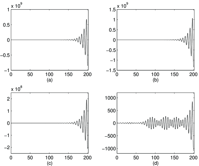
FIG. 1.: Sample of narrow resonance regime results. $\chi_{k}(t)$ is plotted (vertical axis) against dimensionless time (horizontal axis) for a value of $k$ in the first resonance band, $E^{2}=1$, and for $\lambda=0.4$.
(a) No noise is present, $q(t)=0$.
(b) The noise is characterized by $\bar{q}\approx 0.010\,\lambda$, $\Gamma=10$ and $g=0.8$ (large amplitude and large noise frequency).
(c) The noise is characterized by $\bar{q}\approx 0.028\,\lambda$, $\Gamma=1/40$ and $g=0.4$ (small amplitude and small noise frequency).
(d) The noise is characterized by $\bar{q}\approx 0.433\,\lambda$, $\Gamma=1/20$ and $g=0.9$ (large amplitude and small noise frequency). In this case, the mode $k$ is shifted out of the resonance band. This is an example for which the noise is important.

(i) The noise has practically no effect when $\Gamma$, the inverse of its characteristic time, is much bigger than the frequency $\omega$ of the periodic driving function $p(\omega t)$, i.e. when $\Gamma\gg\omega$. This is shown in Figures 1(b) and 2(b) where $\Gamma\gg 1$, and it is consistent with the results of Sections V and VI (see e.g. Eqs. (83) and (84)). On the other hand, if $\Gamma$ is small compared to $\omega$, then the ergodic hypothesis is not satisfied, and the noise may completely alter the efficiency of energy transfer (see e.g. Figures 1(d) and 2(d)).

(ii) In the case of narrow resonance, the noise is effective only if its magnitude is of the same order or larger than the amplitude of $p(\omega t)$, i.e. $g>1/2$. For values of $g$ significantly smaller than $1$ ($g<0.5$, say) the noise is not effective for “central” modes in a resonance band. This result was obtained in Sections III, IV and V and is illustrated by Figure 1(c).

(iii) The presence of noise may lead to a much faster exponential growth of a mode initially in a resonance band. This effect is particularly important in the case of broad resonance (Figure 2(d)).

(iv) After having analyzed the time evolution of $\chi_{k}(t)$ for many different random walks we verified that an important quantity to be considered is $\bar{q}$, the end point distance of $q(t)$ divided by the number of steps, over the total time interval of reheating $t$. Note that $\bar{q}=g\lambda\bar{n}\sim g\lambda/(t\Gamma)^{1/2}$. If $\bar{q}$ is small compared to the amplitude $A$ of $p(\omega t)$, i. e. if $g/(t\Gamma)^{1/2}\ll 1$, then the resonance is preserved. For some very special random walks in the broad resonance regime (see Figure 2(c)) there are specific realizations for which the noise decreases the Lyapunov exponent, but when taking the average over many realizations, agreement with the analytical results is restored.

In order to understand the above results, notice that parametric resonance of a given mode of the field $\chi$ disappears if the noise is able to keep the mode out of the resonance band during a sufficiently large time interval (when compared to the total evolution time).

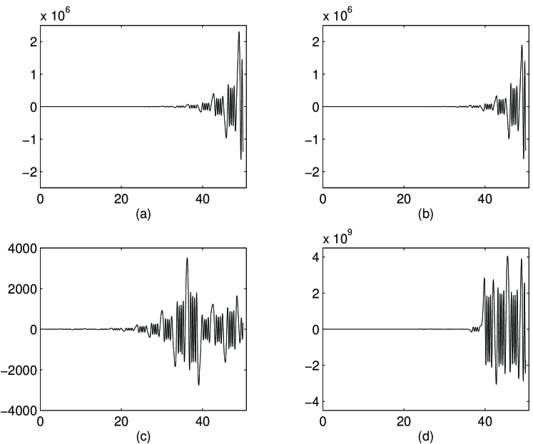
FIG. 2.: Similar plots as in Figure 1, but now for the broad resonance regime. We consider a mode in the tenth resonance band, $E^{2}=100$, and we choose $\lambda=100$.
(a) No noise is present, $q(t)=0$.
(b) The noise is given by $\bar{q}\approx-0.004\,\lambda$, $\Gamma=12.5$ and $g=0.2$ (i.e. large inverse characteristic time and large noise amplitude).
(c) The noise is given by $\bar{q}\approx 0.013\,\lambda$, with the same $\Gamma$ and $g$ as in the case (b).
(d) The noise is given by $\bar{q}\approx-0.025\,\lambda$, $\Gamma=0.2$ and $g=0.30$ (small $\Gamma$ and small noise amplitude). In this example the noise has an important effect. It greatly increases the rate of particle production. In this particular case, the noise $n$ takes on negative values for a few successive time steps, which keeps the mode in an instability region whose Floquet multiplier is larger than without noise. Thus, even though $\bar{q}$ is small, the overall effect is an increased resonance strength due to the very fast exponential growth during a short time interval.

To see exactly what this means let us write the band number $N$ in terms of the parameters of Eq. (85). From the theory of the Mathieu equation we have (neglecting the noise) $N_{o}=|E|$. According to the point (iv) above, the presence of the noise can be approximately taken into account by shifting the value of $E^{2}$ to $E^{2}+g\lambda\bar{n}=E^{2}+\bar{q}/\omega^{2}$. Then, by defining $N^{2}=N_{o}^{2}+\bar{q}/\omega^{2}$ where $N_{o}$ is the band number when the noise is neglected ($N_{o}^{2}=E^{2}$) we obtain

$$\Delta N\equiv N-N_{o}=N_{o}\frac{\bar{q}}{2\omega_{k}^{2}}=N_{o}g{\lambda\over E^{2}}\bar{n}\,.$$ (86)

This result means that for large $N_{o}$, that is to say for modes initially in one of the resonance bands with large band number, even a very small mean noise (when compared to the energy of the mode $\omega_{k}^{2}$) can shift a given mode through several bands and occasionally into a stability band. However, since the same noise is assumed to act independently upon all the modes, it is easy to see that some of the modes initially in a stability band can be shifted to an instability band. This effect is important in the broad resonance regime, where the resonance occurs for $E^{2}\sim\lambda\gg 1$. For instance, in the case of Fig. 2 we have $\lambda/E^{2}=1$, so that $\Delta N=5g\bar{n}$. Then, even for $g\approx 0.1$ there are special samples of the noise that have a significant effect on the resonance of the boson field (a small effect of the noise means $\Delta N\ll 1$) . In particular, for Figs. 2(b) and 2(c) we find $\Delta N\simeq-0.02$ and $\Delta N\simeq 0.08$, respectively.

On the other hand, for small $N_{o}$ in principle the mean noise could be of the order of $\omega_{k}^{2}$ without jumping to the next resonance band. However, this corresponds to the narrow resonance regime $\lambda\equiv\varepsilon\ll 1$, where the width of the instability bands are very narrow and the mode can easily be shifted to a stability band. In fact, for a mode $k$ initially in the center of the first band the mean noise $\bar{q}$ must satisfy $|\bar{q}|/\omega_{k}^{2}<\varepsilon/2$ in order for not to take the mode out of the first resonance band. Notice that $\varepsilon$ is by definition the ratio $A/\omega_{k}^{2}$ so that the (narrow) resonance is preserved as long as $|\bar{q}|$ is smaller than one half of the amplitude $\lambda$ of the periodic driving function $p(\omega t)=\lambda\cos(2t)$. In the case of Fig. 1 we have $\lambda/E^{2}=0.4$, so that $\Delta N=0.4g\bar{n}$, which implies a small effect of the noise even for $g$ of the order of $1$. For instance, in the case of Figs. 1(c) and 1(d) we have respectively $\Delta N\simeq 0.01$ and $\Delta N\simeq 0.08$.

According to the general analysis of Sect. II, ergodic noise always increases the rate of particle production. In the numerical work, however, we find examples where over a small time interval the rate of particle production is decreased as a consequence of the noise. This is manifest in the case of small $\Gamma$ (Figures 1(c), 1(d) and 2(d)). This apparent contradiction disappears once we realize that for small $\Gamma$ and for a finite reheating interval, we are in fact not taking the average of $q(\kappa,t)$ over many realizations in the sample space $\Omega$, but instead choosing only a few special noise functions for each calculation. By the ergodic hypothesis used in Section II, we should expect that numerical results to agree with the exact results only if the reheating time $t$ is very big compared to the characteristic time $T\equiv\Gamma^{-1}$ of the noise. (The time $t$ must be very big, compared to $T$, to ensure that the noise explores all possible realizations in the “noise space”.) This condition is grossly violated for the parameters of Figs. 1c and 1d. There are also cases (see Figure 2(c)) when $\Gamma$ is large but for certain realization of the noise the Lyapunov exponent decreases. In all these cases, however, the mean Lyapunov number over many realizations is larger than the Lyapunov exponent in the absence of noise. It would be of interest to further study the dispersion of the Lyapunov exponents for identical values of the physical parameters.

VIII Conclusions

We have studied some effects of noise on parametric resonance. Specifically, we considered spatially homogeneous noise in the time dependent mass responsible for the parametric resonance instability. Assuming that the noise is ergodic we showed that the presence of the noise leads to strict increase in the rate of particle production. We demonstrated also that the resonance is rather insensitive to the presence of small noise. Under the assumption that the time dependence of the noise can be modeled as a random walk with a characteristic step length, we derived estimates for the amplitude of the noise for which it can be shown that the resonance persists. We demonstrated that even if the dimensionless amplitude of the noise $g$ is of the order 1, resonance is not affected provided the time step $\Gamma^{-1}$ of the noise is sufficiently short. In a subsequent letter${}^{\cite[cite]{[\@@bibref{Number}{ZMCB2}{}{}]}}$ we will extend these results to the more interesting case of spatially inhomogeneous noise.

Appendix

This last section gives an outline of the mathematical results that are used in this work. Complete proofs appear in the literature citations.

Proposition 1:  When $q(t;\kappa)$ is given by a translation invariant ergodic measure $dP(\kappa)$ on $C({\mathbf{R}})$, the limit exists,

$\displaystyle\overline{\mu}=\lim_{N\to\infty}{1\over NT}E(\log\|\Pi_{j=1}^{N}\Phi_{q}(jT,(j-1)T)\|)~{}.$Furthermore, for almost every realization $\kappa$ (with respect to the probability measure $dP(\kappa)$) the individual limits exist,

$\displaystyle\mu(q)=\lim_{N\to\infty}{1\over NT}\log\|\Pi_{j=1}^{N}\Phi_{q}(jT,(j-1)T)\|~{},$and they are equal to $\overline{\mu}$.

The proof of the first statement follows from an argument involving the sequence $e(n)=E(\log\|\Pi_{j=1}^{n}\Phi_{q}(jT,(j-1)T)\|)$ and its subadditive property, $e(n+m)\leq e(n)+e(m)$. The proof of the second statement follows from the subadditive ergodic theorem, [19].

Proposition 2:  The generalized Floquet exponent (Lyapunov exponent) $\mu(q)$ is continuous with respect to $q$ in the topology on $C({\mathbf{R}})$ of uniform convergence on compact sets.

This result and its proof may be found in [17] and [18]; it follows from Sturm - Liouville theory and the nesting property of the Weyl limit circles.

The third qualitative result has to do with a monotonicity property of the generalized Floquet exponent in ergodic systems. Consider the probability space $\Omega=C({\mathbf{R}})$ with two ergodic invariant measures $dP_{1}$ and $dP_{2}$. By Proposition 1 the two associated generalized Floquet exponents $\mu_{1}$ and $\mu_{2}$ are constant almost everywhere on the support of their respective measures. The following result states that the class of problems (6) with positive generalized Floquet exponent is nondecreasing with respect to the support of the measure.

Theorem 3:  (S. Kotani [18])  If ${\mathrm{s}upp}\,(dP_{1})\subseteq{\mathrm{s}upp}\,(dP_{2})$ and $\mu_{1}>0$, then $\mu_{2}>0$.

In our case $dP_{1}$ is supported on the periodic function $p(t)$ and its translates, and $dP_{2}$ will be taken to be the description of the statistics of the realizations $\{p(t)+q(t;\kappa)\}\subseteq C({\mathbf{R}})$. If $q(t)=0$ is a possible realization in the support of the probability measure $dP(\kappa)$, then the support of $dP_{2}$ contains the support of $dP_{1}$. We are therefore in the situation described in Theorem 3.

The final mathematical result of this article is also the central one to our argument. Consider a probability distribution $dA$ on the matrices $\Psi\in{\mathrm{S}L}(2,{\mathrm{R}})$ (in fact the result applies more generally to ${\mathrm{S}L}(n,{\mathrm{R}})$). Let $G_{A}$ be the smallest subgroup of ${\mathrm{S}L}(2,{\mathrm{R}})$ containing the support of $dA$.

Theorem 4:  (Furstenberg, [19])  Suppose that $G_{A}$ is not compact, and that the action of $G_{A}$ on the set of lines in ${\mathrm{R}^{2}}$ has no invariant measure. Then for almost all independent random sequences $\{\Psi_{j}\}_{j=1}^{\infty}\subseteq{\mathrm{S}L}(2,{\mathrm{R}})$ with common distribution $dA$,

$\displaystyle\lim_{N\to\infty}{1\over N}\log(\|\Pi_{j=1}^{\infty}\Psi_{j}\|)=\lambda>0~{}.$Furthermore, for given $v_{1},v_{2}\in{\mathrm{R}^{2}}$, then

$\displaystyle\lim_{N\to\infty}{1\over N}\log(\langle v_{1},\Pi_{j=1}^{\infty}\Psi_{j}v_{2}\rangle)=\lambda$for almost every sequence $\{\Psi_{j}\}_{j=1}^{\infty}$.

In our setting, realizations $\{q(t;\kappa):0\leq t<T\}$ give rise to transfer matrices $\Psi_{q}(T,0)\in{\mathrm{S}L}(2,{\mathrm{R}})$, and the probability measure $dP$ on $C({\mathbf{R}})$ induces a measure $dA$ on ${\mathrm{S}L}(2,{\mathrm{R}})$. We will fulfill the hypotheses of the theorem of Furstenberg for $dA$ by demonstrating that under our conditions on ${\mathrm{s}upp}(dP)$, then $G_{A}={\mathrm{S}L}(2,{\mathrm{R}})$. This will follow if we show that the set of random transfer matrices $\{\Psi_{q}(T,0):q\in{\mathrm{s}upp}(dP)\}$ contains a small neighborhood of the identity in ${\mathrm{S}L}(2,{\mathrm{R}})$, for this must be contained in the support of the induced measure $dA$. In order to analyse this set, observe that the sequence of successive approximations $\{\Psi_{j}(t,0)\}_{j=1}^{\infty}$ gives the Taylor polynomials of the fundamental solution $\Psi(t,0;q)=\Psi_{q}(t,0)$ with respect to $q\in C(0,T)$ about $q(t)=0$. Thus the derivative of the transfer matrix $\Psi(T,0;q)$ with respect to $q(t)$ at zero is given by the first term

$$\delta_{q}\Psi(T,0;0)\cdot r(t)=\int_{0}^{T}\ dt\ \ r(t)\Phi_{0}^{-1}(t)\left(\begin{array}[]{cc}0&0\\ -1&0\end{array}\right)\Phi_{0}(t)~{}.$$ (87)

From (8) and the fact that ${\mathrm{d}et}(\Phi_{0}(t))=1$, this is

$$\delta_{q}\Psi(T,0;0)\cdot r(t) = \int_{0}^{T}\ dt\ \ r(t)\left(\begin{array}[]{cc}\dot{\phi}_{2}&-\phi_{2}\\ -\dot{\phi}_{1}&\phi_{1}\end{array}\right)\left(\begin{array}[]{cc}0&0\\ -1&0\end{array}\right)\left(\begin{array}[]{cc}\phi_{1}&\phi_{2}\\ \dot{\phi}_{1}&\dot{\phi}_{2}\end{array}\right)$$ (94)

$$= \int_{0}^{T}\ dt\ \ r(t)\left(\begin{array}[]{cc}\phi_{1}(t)\phi_{2}(t)&\phi_{2}^{2}(t)\\ -\phi_{1}^{2}(t)&-\phi_{1}(t)\phi_{2}(t)\end{array}\right)~{}~{}.$$ (97)

For $r(t)\in C(0,T)$ the expression $\delta_{q}\Psi(T,0;0)\cdot r$ is in the Lie algebra ${\mathrm{s}l}(2,{\mathrm{R}})$. Taking $r(t)\in{\mathrm{s}upp}(dP)$ in a small neighborhood of zero, if $\delta_{q}\Psi(T,0;0)\cdot r$ spans ${\mathrm{s}l}(2,{\mathrm{R}})$, then by the implicit function theorem the solutions $\Psi(T,0;q)$ will indeed fill a neighborhood of $I\in{\mathrm{S}L}(2,{\mathrm{R}})$. From the structure of (94) the rank of $\delta_{q}\Psi(T,0;0)\cdot r$ is at most three, spanned by $\{\phi_{1}^{2}(t),\phi_{1}(t)\phi_{2}(t),\phi_{2}^{2}(t)\}$, and the question is whether these three components are in all cases linearly independent in $C(0,T)$.

By direct calculation one verifies that products $\psi(t)=\phi_{j}(t)\phi_{k}(t)$ of solutions of equation (3) satisfy themselves a third order differential equation

$${d^{3}\over dt^{3}}\psi=-2({d\over dt}(\omega^{2}+p(t))+(\omega^{2}+p(t)){d\over dt})\psi~{}.$$ (98)

At $t=0$ the Wronskian for (98) is

$$\Delta(t)\Bigl{|}_{t=0}=\left(\begin{array}[]{ccc}\phi_{1}^{2}&\phi_{1}\phi_{2}&\phi_{2}^{2}\\ \dot{(\phi_{1}^{2})}&\dot{(\phi_{1}\phi_{2})}&\dot{(\phi_{2}^{2})}\\ \ddot{(\phi_{1}^{2})}&\ddot{(\phi_{1}\phi_{2})}&\ddot{(\phi_{2}^{2})}\\ \end{array}\right)=\left(\begin{array}[]{ccc}1&0&0\\ 0&1&0\\ -2(\omega^{2}+p(t))&0&\ \ \ \ 2\\ \end{array}\right)~{},$$ (99)

therefore $\det(\Delta(t))=2$ for all $t$, and the three functions $\phi_{1}^{2}(t),\phi_{1}(t)\phi_{2}(t),\phi_{2}^{2}(t)$ form a linearly independent set.

Suppose by way of contradiction that the rank of $\delta_{q}\Psi(T,0;0)\cdot r$ is less than three, so that there is a linear relationship

$\displaystyle c_{1}\phi_{1}^{2}+c_{2}\phi_{1}(t)\phi_{2}(t)+c_{3}\phi_{2}^{2}(t)=0~{}.$Taking two derivatives, this implies that $(c_{1},c_{2},c_{3})^{t}$ is a null vector for $\Delta(t)$, contradicting the above assertion of independence.

It is therefore only necessary that ${\mathrm{s}pan}(\phi_{1}^{2}(t),\phi_{1}(t)\phi_{2}(t),\phi_{2}^{2}(t))\cap{\mathrm{s}upp}(dP)$ contain a small neighborhood of the origin in order that

${\mathrm{r}ank}\{\delta_{q}\Psi(T,0;0)\cdot r:r(t)\in{\mathrm{s}upp}(dP)\cap B_{\epsilon}(0)\}=3$.

This is surely satisfied for any periodic potential $p(t)$ if $B_{\epsilon}(0)\subseteq{\mathrm{s}upp}(dP)$, which is our hypothesis.

REFERENCES

-
[1]
J. Traschen and R. Brandenberger, Phys. Rev. D42,
2491 (1990);
A. Dolgov and D. Kirilova, Sov. Nucl. Phys. 51, 172 (1990). - [2] L. Kofman, A. Linde and A. Starobinsky, Phys. Rev. Lett. 73, 3195 (1994), hep-th/9405187.
- [3] Y. Shtanov, J. Traschen and R. Brandenberger, Phys. Rev. D51, 5438 (1995), hep-ph/9407247.
- [4] L. Kofman, A. Linde and A. Starobinsky, “Towards the Theory of Reheating After Inflation”, hep-ph/9704452 (1997).
-
[5]
M. Yoshimura, Prog. Theor. Phys. 94, 873 (1995);
D. Boyanovsky, H. de Vega and R. Holman, “Erice Lectures on Inflationary Reheating”, hep-ph/9701304, and refs. therein;
D. Kaiser, Phys. Rev. D53, 1776 (1996). -
[6]
W. Press, Phys. Scr. 21, 702 (1980);
G. Chibisov and V. Mukhanov, “Galaxy Formation and Phonons”, Lebedev preprint No. 162 (1980), Mon. Not. R. Astr. Soc. 200, 535 (1982);
V. Lukash, Pis’ma Zh. Eksp. Teor. Fiz. 31, 631 (1980);
V. Mukhanov and G. Chibisov, JETP Lett. 33, 532 (1981);
V. Mukhanov and G. Chibisov, Sov. Phys. JETP 56, 258 (1982);
K. Sato, Mon. Not. R. Astr. Soc. 195, 467 (1981). - [7] R. Allahverdi and B. Campbell, Phys. Lett. B395, 169 (1997), hep-ph/9606463.
-
[8]
S. Khlebnikov and I. Tkachev, Phys. Rev. Lett.
77, 219 (1996);
S. Khlebnikov and I. Tkachev, Phys. Lett. B390, 80 (1997), hep-ph/9608458. - [9] T. Prokopec and T. Roos, Phys. Rev. D55, 3768 (1997), hep-ph/9610400.
- [10] M. Hotta, I. Joichi, S. Matsumoto and M. Yoshimura, Phys. Rev. D55, 4614 (1997), hep-ph/9608374.
- [11] R. Brandenberger, “Particle Physics Aspects of Modern Cosmology”, in “Field Theoretical Methods in Fundamental Physics”, ed. C. Lee (Minumsa Publ., Seoul, 1997); hep-ph/9701276.
- [12] N. Bogoliubov and Y. Mitropolsky, “Asymptotic Methods in the Theory of Nonlinear Oscillations” (Hindustan Publishing, Delhi, 1961).
- [13] H. Hoschstadt, “The Functions of Mathematical Physics”, Dover Pub. (1986), p 284.
- [14] R. Kress. “Linear Integral Equations”, Springer-Verlag (1989), p 33.
- [15] A. Rabenstein, “Introduction to Ordinary Differential Equations”, Academic Press, N.Y. (1966), p. 24.
- [16] V. Zanchin, A. Maia, W. Craig and R. Brandenberger, in preparation (1997).
- [17] R. Carmona and J. Lacroix, “Spectral theory of random Schrödinger operators” (1990) Birkhäuser, Boston. See p 198 for the proof of existence of the Floquet exponents and p 200 for the proof of the Furstenberg’s theorem.
- [18] S. Kotani, “Support theorems for random Schrödinger operators”, Commun. Math. Physics 97 (1985), pp. 443 - 452.
- [19] L. Pastur and A. Figotin, “Spectra of random and almost-periodic operators”, (1991) Springer Verlag, Berlin. See p 256 for theory of generalized Floquet(Lyapunov) exponents and p 344 for the Furstenberg’s theorem.