Neutrino Masses and Flavour Symmetry

Abstract

The problem of neutrino masses and mixing angles is analysed in a class of supersymmetric grand unified models, with $SO(10)$ gauge symmetry and global $U(2)$ flavour symmetry. Adopting the seesaw mechanism for the generation of the neutrino masses, one obtains a mass matrix for the left–handed neutrinos which is directly related to the parameters of the charged sector, while the unknown parameters of the right–handed Majorana mass matrix are inglobed in a single factor.

PACS 12.10	–	Unified Field Theories and Models.
PACS 12.15.Ff	–	Quark and Lepton Masses and Mixing.

1 Introduction

The problem of neutrino masses is of great importance both for particle physics and astrophysics. However, it is still an open problem: on one hand, the experimental indications of neutrino oscillations would indicate non-vanishing neutrino masses and mixing angles; on the other hand, the predictions for such quantities are strongly dependent on the specific theoretical assumptions. Some of the main questions of neutrino physics should be resolved by the new generations of oscillation experiments which are under way (for a review see ref.[1]), and then one would be able to discriminate among the different theoretical schemes.

While the minimal version of the Standard Model (SM) accomodates only massless neutrinos, several different extensions have been proposed, in which neutrino masses and mixing are generated. In the present note, we shall adopt the simplest form of the seesaw mechanism [2], in which right-handed neutrinos are introduced and both Dirac $M_{D}\equiv M_{LR}$ and Majorana $M_{M}\equiv M_{RR}$ mass matrices are generated. As a consequence, the light neutrino masses are of the type $M_{\nu}=M_{D}M_{M}^{-1}M_{D}^{T}$. While $M_{D}$ can be connected in grand unified schemes to the charged lepton masses, the Majorana mass matrix $M_{M}$ appears to be decoupled, in general, from the charged sector.

Many theoretical investigations have been devoted to the analysis of the mass spectrum of quarks and charged leptons. Most of them are based on supersymmetric grand unified models, thus keeping the nice features of gauge unification [3] and of the equality of the b-quark and $\tau$-lepton masses at the unification scale. The pattern of quark and lepton masses is characterized by a strong hierarchy, which in the case of down-type quarks can be approximately described by

$$m_{d}:m_{s}:m_{b}\approx\lambda^{4}:\lambda^{2}:1,$$ (1)

where $\lambda\simeq 0.22$ is the Cabibbo angle, and by

$$m_{u}:m_{c}:m_{t}\approx\lambda^{8}:\lambda^{4}:1,$$ (2)

for the up-type quarks. The case of the charged leptons is roughly similar to (1). Such hierarchies lead to the ansatz of zero textures, first employed by Fritzsch [4] and then analysed in detail for the Yukawa matrices by Ramond, Roberts and Ross [5]. These textures suggested the introduction of an underlying “family” symmetry, and several schemes were proposed based on discrete or continuous groups (we refer for details to the review papers [6]). The Abelian group $U(1)$ (either global or local) has been one of the most favoured: it can be interpreted as the remnant of a larger “family” or “flavour” group $U(3)\subset U(45)$, which acts among the three fermion families, or among all the different flavours.

An approximate flavour $U(2)$ symmetry has recently been proposed [7,8] as an interesting framework for understanding the role of flavour breaking in supersymmetric theories. It is more useful than the complete $U(3)$ symmetry, which is badly broken by the large top-quark mass, and it is more predictive than the Abelian $U(1)$ symmetry. While solving the supersymmetric flavour-changing problem, it leads to interesting relations among the masses and mixing angles, some of which appear to be well satisfied [9]. Specific models based on $SU(5)\otimes U(2)$ and $SO(10)\otimes U(2)$ have been analysed [9,10].

More recently, the analysis based on the $U(2)$ flavour symmetry has been extended to the neutrino sector [11], with some interesting results for the neutrino phenomenology. The model, which is based on $SU(5)\otimes U(2)$ will be briefly discussed in the following; in alternative, we present here a class of models based on the symmetry $SO(10)\otimes U(2)$ which exhibit an important advantage. In fact, one can show that the light neutrino mass matrix can be directly related to the parameters of the quark and charged lepton mass matrix, while the unknown parameters of the right-handed neutrino Majorana mass matrix are inglobed in a single factor.

In Section 2, we outline the general features of the $U(2)$ flavour symmetry models. In Section 3 we review what has been done in the frame of $SU(5)\otimes U(2)$ scheme, both for the charged fermions and for the neutrinos; in Section 4 we go to $SO(10)\otimes U(2)$ and describe our results for the neutrino sector; finally, we draw our conclusions.

2 Fermion masses in $U(2)$ flavour symmetry models

While we refer to the review papers [6] for the information about the different approaches adopted for the problem of the fermion mass hierarchies, we outline here the theoretical framework for the specific case of the $U(2)$ flavour symmetry [7,8].

Remaining, for the moment, at the level of the Minimal Supersymmetric Standard Model (MSSM), the internal symmetry group is specified by:

$$G^{int}=G^{int}_{SM}\otimes U(2).$$ (3)

We denote by $\psi$ all the chiral superfields which include the whole fermion sector of the SM, and by $h$ the two Higgs doublets $h_{u}$ and $h_{d}$; they are assigned to the $U(2)$ representations as follows: $\psi=\psi_{a}+\psi_{3}={\bf 2}+{\bf 1}\;(a=1,2)$ and $h={\bf 1}$.

The Yukawa interactions can be obtained from an operator expansion of the superpotential in an effective theory, in terms of a set of fields $f$, called “flavons”, which develop vacuum expectation values (vevs) breaking the $U(2)$ symmetry:

$$W={[\psi h(1+f/M+f^{2}/{M^{2}}+...)\psi]}_{F}.$$ (4)

and $M$ is the cut-off of the effective theory.
The flavons can be assigned only to the ${\bf 2}$ and ${\bf 2}\times{\bf 2}={\bf 3}_{s}+{\bf 1}_{a}$ representations of $U(2)$ ($\phi^{a}={\bf 2},S^{ab}={\bf 3}_{s},A^{ab}={\bf 1}_{a}$) and the effective superpotential becomes to order $f/M$:

$$W=\psi_{3}h\psi_{3}+{1\over M}\psi_{3}h\phi^{a}\psi_{a}+{1\over M}\psi_{a}h(S^{ab}+A^{ab})\psi_{b}.$$ (5)

It is assumed that the symmetry $U(2)$ is broken spontaneously in two steps by the vevs $\langle\phi^{2}\rangle$, $\langle S^{22}\rangle$ and $\langle A^{12}\rangle$:

$$U(2)\buildrel\epsilon\over{\longrightarrow}U(1)\buildrel\epsilon^{\prime}\over{\longrightarrow}\O.$$ (6)

The Yukawa matrices ($\lambda^{U,D}$ for the up–, down–type quarks and $\lambda^{E}$ for the charged leptons) are given by the same expression:

$$\lambda\sim\left(\begin{array}[]{ccc}0&\epsilon^{\prime}&0\\ -\epsilon^{\prime}&\epsilon&\epsilon\\ 0&\epsilon&1\end{array}\right)$$ (7)

where $\epsilon\simeq\epsilon_{S}\simeq\epsilon_{\phi}\ll 1$ ($\epsilon_{S}=\langle S^{22}\rangle/M$ , $\epsilon_{\phi}=\langle\phi^{2}\rangle/M$), and $\epsilon^{\prime}=\langle A^{12}\rangle/M\ll\epsilon$. This structure is satisfactory from the phenomenological point of view if [9]:

$$\epsilon\approx m_{s}/m_{b}$$ (8)

$$\epsilon^{\prime}\approx\sqrt{\frac{m_{d}m_{s}}{{m_{b}}^{2}}}.$$ (9)

However, there are some difficulties related to the fact that the hierarchy in the up-like quark sector is stroger than in the down-like quark and charged lepton sectors, which can be exemplified by:

$$m_{\tau}\approx m_{b}\ll m_{t}.$$ (10)

These difficulties could be overcomed by discriminating between $\lambda^{U}$ and $\lambda^{D}\approx\lambda^{E}$, and by imposing that the $\lambda^{U}_{22}$ and $\lambda^{U}_{21}$ entries vanish at order $\epsilon$ and $\epsilon^{\prime}$. These features can be realized in grand unified models, as will be shown in the next sections.

We note that the problem of FCNC, which arises in general in supersymmetric theories due to the presence of soft breaking terms, can find a natural solution in the $U(2)$ flavour symmetry model [7]. The suppression of FCNC requires, in fact, mass degeneracy of the sfermions of the first two families: in the $U(2)$ model the splitting is indeed very small (of order $\epsilon^{2}$). On the other hand, the splitting between the third and the two lighter families of sfermions could give rise to appreciable contributions for observables like the $\mu\rightarrow e+\gamma$ decay and the $CP$-violating parameter $\epsilon_{K}$ and this would be an interesting signature of the model [7].

3 The $SU(5)\otimes U(2)$ model

A way of suppressing the $\lambda^{U}_{22}$ and $\lambda^{U}_{21}$ entries, keeping at the same time the corresponding $\lambda^{D,E}_{22}$ and $\lambda^{D,E}_{21}$ different from zero, can be realized in the frame of the $SU(5)$ grand unification.

With the usual assignements of a fermion family to the superfield $T_{i}({\bf 10})+\bar{F}_{i}({\bf\bar{5}})$, and of the two Higgs doublets to the superfields $H_{u}({\bf 5})$ and $H_{d}({\bf\bar{5}})$, the superpotential (5) is replaced by:

$$W_{(5)} = T_{3}H_{u}T_{3}+T_{3}H_{d}\bar{F}_{3}+$$ (11)

$${1\over M}(T_{3}H_{u}\phi^{a}T_{a}+T_{3}H_{d}\phi^{a}\bar{F}_{a}+\bar{F}_{3}\phi^{a}H_{d}T_{a})+$$

$${1\over M}[T_{a}(S^{ab}+A^{ab})H_{u}T_{b}+T_{a}(S^{ab}+A^{ab})H_{d}\bar{F}_{b}].$$

Here and in the following, an arbitrary complex constant of order $O(1)$ is implied for each term of the superpotential. The fields $\phi^{a}$ can be assigned either to $\bf 1$ or to $\bf 24$ and a convenient choice for the other flavons is

$$S^{ab}={\bf 75}\;\;\;\;\;\hbox{and}\;\;\;\;\;A^{ab}={\bf 1}.$$ (12)

In fact, as shown in [9], the above assignement, which implies that the terms $S^{ab}H_{u}$ and $A^{ab}H_{u}$ transform, respectively, as ${\bf 45}$ and ${\bf 5}$, guarantees the vanishing of $\lambda^{U}_{22}$ and $\lambda^{U}_{21}$ at order $\epsilon$ and $\epsilon^{\prime}$.

In order to obtain a non vanishing contribution for the $m_{u}$ mass at higher order, one has to introduce an extra familon $\Sigma_{Y}$ in the representation ${\bf 24}\otimes{\bf 1}$ of $SU(5)\otimes U(2)$, with a vev in the direction of the hypercharge $Y$ with value $\langle\Sigma_{Y}\rangle/M\simeq\rho\simeq 0.02$.
The additional terms in the superpotential are:

$$W^{\prime}_{(5)}={1\over M^{2}}T_{a}[\phi^{a}\phi^{b}+(S^{ab}+A^{ab})\Sigma_{Y}]H_{u}T_{b}$$ (13)

which generate the contributions $\lambda^{U}_{22}=O(\epsilon\rho)$, and $\lambda^{U}_{12}=O(\epsilon^{\prime}\rho)$.

Finally, one can write for the Yukawa matrices

$$\lambda^{U} = \lambda\pmatrix{0&\epsilon^{\prime}\rho&0\cr-\epsilon^{\prime}\rho&\epsilon\rho^{\prime}&x_{u}\epsilon\cr 0&y_{u}\epsilon&1\cr}$$ (14)

$$\lambda^{D,E} = \xi\pmatrix{0&\epsilon^{\prime}&0\cr-\epsilon^{\prime}&(1,-3)\epsilon&(x_{d},x_{e})\epsilon\cr 0&(y_{d},y_{e})\epsilon&1\cr}$$ (15)

where the complex coefficients $x_{u},x_{d},x_{e},y_{u},y_{d},y_{e}$ are of order 1, and $\rho^{\prime}=O(1)\rho$. Moreover, to account for the different hierarchies (1) and (2) one has to take $\xi<<\lambda$, which can be realized by assuming that the light Higgs (in the unified multiplet $H_{d}$) which couples to the D/E sector contains a small component (of order $m_{b}/m_{t}$) of the Higgs doublet [9].
Disregarding the unknown factors of order 1, the matrices (14) and (15) depend only on 4 small parameters: $\rho\simeq\epsilon\simeq\xi\simeq 0.02$ and $\epsilon^{\prime}\simeq 0.004$.
With this approximation one can relate the 13 observables of the fermion sector by means of 9 approximate relations; in fact, 5 of them are precise relations [9].

So far neutrinos have been considered strictly massless. Let us now add a right–handed neutrino superfield $\nu_{i}$ to each family, singlet under $SU(5)$ and transforming as

$$\nu_{i}=(\nu_{a},\nu_{3})=({\bf 2},{\bf 1})$$ (16)

under $U(2)$.
Correspondingly, the superpotential contains the additional terms:

$$W^{D}_{(5)} = \bar{F}_{3}H_{u}\nu_{3}+{1\over M}[\bar{F}_{3}\phi^{a}H_{u}\nu_{a}+\bar{F}_{a}\phi^{a}H_{u}\nu_{3}+\bar{F}_{a}A^{ab}H_{u}\nu_{b}]$$ (17)

$$+{1\over M^{2}}\bar{F}_{a}(\phi^{a}\phi^{b}+S^{ab}\Sigma_{Y})H_{u}\nu_{b}.$$

They produce a Dirac mass matrix of the form:

$$\lambda^{\nu}_{D}\sim\pmatrix{0&\epsilon^{\prime}&0\cr-\epsilon^{\prime}&\rho\epsilon&\epsilon\cr 0&\epsilon&\rho\cr}$$ (18)

where only the order of magnitude is indicated for each entry.
The Majorana mass matrix for the right–handed neutrinos is generated by the superpotential

$$W^{M}_{(5)}=\lambda_{M}\nu_{3}\nu_{3}+{\lambda_{M}\over M}[\nu_{a}\phi^{a}(1+{\Sigma_{Y}\over M})\nu_{3}+\nu_{a}({\phi^{a}\phi^{b}\over M})\nu_{b}].$$ (19)

We note that terms containing $A^{ab}$ and $S^{ab}$ are not allowed by symmetry reasons and by the assignement (12). Since the superfield $\phi^{a}$ can be assigned either to ${\bf 1}$ or ${\bf 24}$, two choices are possible for the Majorana mass matrix:

$$\lambda_{M}^{(1)} \sim \lambda_{M}\pmatrix{0&0&0\cr 0&\epsilon^{2}&\epsilon\cr 0&\epsilon&1\cr}$$ (20)

$$\lambda_{M}^{(24)} \sim \lambda_{M}\pmatrix{0&0&0\cr 0&\epsilon^{2}&\rho\epsilon\cr 0&\rho\epsilon&0\cr}.$$ (21)

Similar results are presented in ref. [11].
The Majorana mass matrices obtained from (19) have zero determinant, thus preventing the use of the seesaw mechanism. A solution to this problem can be obtained with the introduction of other flavons in the representations $\bf 1$ or ${\bf 3}_{s}$ of $U(1)$, like $\phi^{a}$ or $S^{ab}$, but with non–vanishing vev’s along the directions $\langle\phi^{1}\rangle$ or $\langle S^{12}\rangle$.

However, this approach is rather dangerous in $SU(5)$, since these flavons should be assigned to the representation 1 or 24 of the gauge group, and then they would couple to all the other fermion fields, spoiling the results obtained for the Yukawa matrices and for the FCNC suppression.
In the quoted ref. [11], a solution with $\langle S^{11}\rangle=\langle S^{12}\rangle=0$ and $\langle\phi^{1}\rangle\leq\epsilon^{\prime}$ is considered to be compatible with the present phenomenology of the quark sector.

In the next section, we propose an alternative approach based on the $SO(10)\otimes U(2)$ symmetry.

4 Models based on $SO(10)\otimes U(2)$

In the supersymmetric models based on the gauge group $SO(10)$ the chiral superfield $\psi_{i}$ contains all fundamental fermions, including the right handed neutrinos (16). The field $\psi_{i}$ and the Higgs fields transform under $SO(10)\otimes U(2)$ as follows:

$$\psi_{i} = \psi_{a}+\psi_{3}={\bf 16}\otimes({\bf 2}\oplus{\bf 1})\;\;(a=1,2)$$ (22)

$$H = h_{u}+h_{d}={\bf 10}\otimes{\bf 1}.$$ (23)

To first order in the familon fields, the superpotential becomes:

$$W_{(10)}=\psi_{3}H\psi_{3}+{1\over M}[\psi_{3}\phi^{a}H\psi_{a}+\psi_{a}(S^{ab}+A^{ab})H\psi_{b}]$$ (24)

where $\phi^{a}$, $S^{ab}$ and $A^{ab}$ belong to the $SO(10)$ representations 1, 45, 54 or 210.

In the following, we consider in detail two different classes of models, which were analysed in ref. [9] in connection with the charged fermion sector. Here we limit ourselves to specify only the main ingredients referring to [9] for details.

I. The first class of $SO(10)$ models consists in a direct extension of the $SU(5)$ model described in the previous sections. One makes the following correspondence between $SU(5)$ and $SO(10)$ flavons:

$$S^{ab}({\bf 75}) \rightarrow S^{ab}({\bf 210})$$ (25)

$$A^{ab}({\bf 1}) \rightarrow A^{ab}({\bf 45})$$ (26)

$$\phi^{a}({\bf 1},{\bf 24}) \rightarrow \phi^{a}({\bf 45})$$ (27)

$$\Sigma_{Y}({\bf 24}) \rightarrow \Sigma_{Y}({\bf 45})$$ (28)

and the vevs of the $SO(10)$ fields have to be taken in the same directions of vev’s of the corresponding $SU(5)$ fields.

With the superpotential (24), the entries $\lambda^{U}_{22}$ and $\lambda^{U}_{12}$ are suppressed to first order in $\langle f\rangle/M$, so that it is replaced by

$$W^{I}_{(10)}=W_{(10)}+W^{\prime}_{(10)}$$ (29)

where the additional terms

$$W^{\prime}_{(10)}={1\over M^{2}}\psi_{a}[\phi^{a}\phi^{b}+(S^{ab}+A^{ab})\Sigma_{Y}]H\psi_{b}$$ (30)

are included, in analogy to what done in $SU(5)$, to produce higher order contributions to $m_{u}$.

The Yukawa matrices obtained from (29) have the same expression of (14) and (15); the only difference being that the assignement of $\phi^{a}({\bf 45})$ to a single representation reduce the number of the independent parameters $x_{a}$ and $y_{a}\;(a=u,d,e)$.
In table 1 we show the order of magnitude obtained for the charged fermion masses, and indicate the flavons which give non–vanishing contributions.

mass	$\bf O()$	flavons
$m_{b},m_{\tau}$	$1$	$1$
$m_{t}$	$1$	$1$
$m_{s},m_{\mu}$	$\epsilon$	$\phi^{a},S^{ab}$
$m_{c}$	$\rho\epsilon$	$\phi^{a},S^{ab}\sum_{Y}$
$m_{d},m_{c}$	$\epsilon^{\prime}$	$A^{ab}$
$m_{u}$	$\rho\epsilon^{\prime}$	$A^{ab}\sum_{Y}$

Table 1

In the present case, also the neutrino Dirac mass matrix is generated by the superpotential (29), which it is given by:

$$\lambda^{\nu I}_{D}=\lambda\pmatrix{0&\epsilon^{\prime}&0\cr-\epsilon^{\prime}&\rho^{\prime}\epsilon&x_{\nu}\epsilon\cr 0&y_{\nu}\epsilon&1\cr}.$$ (31)

The situation is different for the right–handed Majorana mass matrix, since the product decomposition ${\bf 16}\otimes{\bf 16}$ does not contain the identity representation 1. In fact, a term $\nu_{R}\nu_{R}$ would violate the $U(1)_{X}$ symmetry included in $SO(10)$. This term can be generated with the inclusion of flavons in the representation $\overline{\bf 126}$, and by assuming that their vev’s lies in the direction of the $SU(5)$ singlet with $X=-10$.
The following choices are possible:

$$L = \overline{\bf 126}\otimes{\bf 1}$$ (32)

$$L^{a} = \overline{\bf 126}\otimes{\bf 2}$$ (33)

$$L^{ab} = \overline{\bf 126}\otimes{\bf 3}_{s}$$ (34)

and their contributions to the superpotential are given by

$$\psi_{3}L\psi_{3}+\psi_{a}L^{a}\psi_{3}+\psi_{a}L^{ab}\psi_{b}$$

$$+{1\over M}[\psi_{a}\phi^{a}(1+{\Sigma_{Y}\over M})L\psi_{3}+\psi_{a}(S^{ab}+A^{ab}+{\phi^{a}\phi^{b}\over M})L\psi_{b}].$$ (35)

Keeping only $L$ one gets Majorana mass matrices similar to those obtained in the $SU(5)$ case, i.e. (20,21):

$$\langle\Phi^{a}(45)\rangle \sim ({\bf 1},0)\longrightarrow\lambda_{M}\pmatrix{0&0&0\cr 0&\bar{x}\bar{\epsilon}^{2}&\bar{\epsilon}\cr 0&\bar{\epsilon}&1\cr}$$ (36)

$$\langle\Phi^{a}(45)\rangle \sim ({\bf 24},0)\longrightarrow\lambda_{M}\pmatrix{0&0&0\cr 0&\bar{x}\bar{\epsilon}^{2}&\bar{\rho}\bar{\epsilon}\cr 0&\bar{\rho}\bar{\epsilon}&1\cr}$$ (37)

where (,) refers to the $SU(5)\otimes U(1)_{X}$ content and $\bar{\epsilon}\sim\epsilon$, $\bar{\rho}\sim\rho$, $\bar{x}\sim O(1)$. The terms containing $L^{a}$ and $L^{ab}$ generate Majorana mass matrix of the form

$$M_{M}=\lambda_{M}\pmatrix{\bar{x}_{11}&\bar{x}_{12}&\bar{x}_{1}\cr\bar{x}_{12}&\bar{x}_{22}&\bar{x}_{2}\cr\bar{x}_{1}&\bar{x}_{2}&0\cr}$$ (38)

where we have used the notation: $\langle L^{ab}\rangle/\lambda_{M}=\bar{x}_{ab}\sim O(1)$ and $\langle L^{a}\rangle/\lambda_{M}=\bar{x}_{a}\sim O(1)$.

In order to constrain the Majorana mass matrix which, in general, would be the sum of (38) and either (36) or (37), we introduce the minimum set of $L$–type flavons, and assume that each them develops a single vev. To avoid vanishing determinant, we need always two kinds of flavons, such as $(L,L^{a})$, $(L,L^{ab})$ or $(L^{a},L^{ab})$. Taking into account the two possibilities (36) and (37), one can build 8 different kinds of matrices.

II. We consider here a second class of models [9] which are based on $SO(10)$ but that are not reducible to the $SU(5)$ models. The superpotential is given by (24) and the question related to the suppression of the $\lambda^{U}_{22}$ and $\lambda^{U}_{12}$ entries is solved, in the present case, making use of the specific structure of the $SO(10)$ representations.

The flavons are now assigned only to representations ${\bf 45}$ or ${\bf 1}$:

$$\phi^{a} \longrightarrow {\bf 45}$$ (39)

$$S^{ab} \longrightarrow {\bf 45}$$ (40)

$$A^{ab} \longrightarrow {\bf 1}\;\hbox{or}\;{\bf 45}$$ (41)

Different choices for the vev’s of ${\bf 45}$ are possible, leading to alternative solutions of the problems.

   a)

The vanishing of $\lambda^{U}_{22}$ can be obtained by assuming $\langle S^{ab}\rangle={\bf 45}_{B-L}$. The operator $\psi_{a}S^{ab}H\psi_{b}$ in (24) vanishes identically because (B–L) has opposite value for isospin doublets and singlets. In this case also $\lambda^{D,E}_{22}$ are suppressed.

   b)

The vanishing of $\lambda^{U}_{12}$ can be obtained with either $A^{ab}={\bf 1}$ or $A^{ab}={\bf 45}$. With the first choice the operator $\psi_{a}A^{ab}H\psi_{b}$ is suppressed by symmetry reasons, but in this case one gets also $\lambda^{D,E}_{12}=0$. With the second choice, the vev is taken along the $X$–direction; since $X(Q_{L})=X(u^{c}_{R})$, one gets $\lambda^{U}_{12}=0$ and $\lambda^{D,E}_{12}=O(\epsilon^{\prime})$.

   c)

Terms $\lambda^{D,E}_{22}=O(\epsilon)$ and $\lambda^{D,E}_{12}=O(\epsilon^{\prime})$ can be obtained by introducing also a flavon $\Sigma_{X}({\bf 45})$ with vev along the $X-$direction. The higher order contributions to $\lambda^{U}_{22}$ and $\lambda^{U}_{12}$ require the additional terms (30) with the inclusion also of $\Sigma_{X}$. We do not reproduce here the terms of the superpotential which contain $\Sigma_{X}$, given explicity in ref. [9].

Also in this class of model the matrix $\lambda^{U}$ has the same form of (14); there is some change of sign in $\lambda^{E}$, and the explicit expression will be given later.
For the Dirac neutrino mass matrix, one obtains

$$\lambda^{\nu II}_{D}=\lambda\pmatrix{0&-2\epsilon^{\prime}&0\cr 2\epsilon^{\prime}&6\epsilon&x_{\nu}\epsilon\cr 0&y_{\nu}\epsilon&1\cr}$$ (42)

where the parameters $x_{\nu}$ and $y_{\nu}$ depend on the direction of the vev of $\phi^{a}(45)$.
The analysis of the right handed Majorana mass matrix is similar to that performed for the models of the first class; the contribution of the $L$ field is now given by

$$\lambda_{M}\pmatrix{0&0&0\cr 0&\bar{y}\bar{\epsilon}&\bar{\epsilon}\cr 0&\bar{\epsilon}&1\cr}$$ (43)

with $\bar{y}\sim O(1)$.
In the present case, with the inclusions of the possible pairs $(L,L^{a})$, $(L,L^{ab})$ and $(L^{a},L^{ab})$, one gets 5 different kinds of Majorana matrices.

Before discussing the specific properties of the different solutions for the neutrino masses, we collect the Yukawa matrices obtained for the quarks and charged leptons in the two classes I and II:

$$\lambda^{U} = \lambda\pmatrix{0&\epsilon^{\prime}\rho&0\cr-\epsilon^{\prime}\rho&\epsilon\rho^{\prime}&x_{u}\epsilon\cr 0&y_{u}\epsilon&1\cr}$$ (44)

$$\lambda^{(D,E)} = \xi\pmatrix{0&(1,\pm 1)\epsilon^{\prime}&0\cr(1,\mp 1)\epsilon^{\prime}&(1,\mp 3)\epsilon&(x_{d},x_{e})\epsilon\cr 0&(y_{d},y_{e})\epsilon&1\cr}$$ (45)

where the upper and lower signs in (45) refer to class I and II, respectively. It can be shown that the fermion masses and mixing depend on 9 independent real parameters of the 24 introduced in (44, 45), so that 4 precise predictions among the 13 physical quantities are obtained [9]. The independent parameters can be expressed in terms of the physical quantities; in particular one gets $\lambda\sim m_{t},\xi\sim m_{b}\sim m_{\tau},$ and the two relations given in (8) and (9).

The neutrino Dirac mass matrices for the two classes I and II, are explicity:

$$m_{D}^{I,II}=m_{t}\pmatrix{0&(1,-2)\epsilon^{\prime}&0\cr(-1,2)\epsilon^{\prime}&(\rho^{\prime},6)\epsilon&x_{\nu}\epsilon\cr 0&y_{\nu}\epsilon&1\cr}$$ (46)

and the effective neutrino mass matrix becomes

$$M^{I,II}_{\nu}=m^{I,II}_{D}(M^{I,II}_{M})^{-1}(m_{D}^{I,II})^{T}.$$ (47)

The quantities $x_{\nu},y_{\nu}$ are model dependent, but they can be expressed in terms of $x_{a}$ and $y_{a}$ $(a=u,d,c)$, so that the Dirac matrices are strictly linked to the charged fermion sector. On the other hand, the Majorana matrices depend on arbitrary parameters. As noted previously, there are different solutions for $M_{M}$ in both classes; however, in all cases one can write

$$M_{\nu}^{(I,II)}=\langle m_{\nu}\rangle\;\lambda_{\nu}^{(I,II)}$$ (48)

where $\langle m_{\nu}\rangle$ depend on $\lambda_{M}$ and possibly on other parameters of the Majorana matrix, while the $\lambda_{\nu}$ matrices determine the neutrino masses and mixing hierarchies.

It is important to point out that there are three solutions (one in the first class, and two in the second) which, aside from a common factor, do not depend on the parameters of the Majorana matrices. Leaving out a factor $O(1)$, the three solutions can be written as follows:

$$\begin{array}[]{lcl}M^{I}_{M1}=\lambda_{M}\pmatrix{0&0&\bar{x}_{1}\cr 0&\bar{x}\bar{\epsilon}^{2}&\bar{\rho}\bar{\epsilon}\cr\bar{x}_{1}&\bar{\rho}\bar{\epsilon}&1\cr}&\Rightarrow&M^{I}_{\nu 1}\simeq\displaystyle{m_{t}^{2}\over\lambda_{M}}\pmatrix{\eta^{2}&\rho^{\prime}\eta&y_{\nu}\eta\cr\rho^{\prime}\eta&\rho^{\prime 2}&y_{\nu}\rho^{\prime}\cr y_{\nu}\eta&y_{\nu}\rho^{\prime}&y_{\nu}^{2}\cr}\\ &&\\ M^{II}_{M2}=\lambda_{M}\pmatrix{0&0&\bar{x}_{1}\cr 0&\bar{y}\bar{\epsilon}&\bar{\epsilon}\cr\bar{x}_{1}&\bar{\epsilon}&1\cr}&\Rightarrow&M^{II}_{\nu 2}\simeq\displaystyle{m^{2}_{t}\over\lambda_{M}}\pmatrix{4\eta&-12\epsilon^{\prime}&-2y_{\nu}\epsilon^{\prime}\cr-12\epsilon^{\prime}&36\epsilon&6y_{\nu}\epsilon\cr-2y_{\nu}\epsilon^{\prime}&6y_{\nu}\epsilon&y^{2}_{\nu}\cr}\\ &&\\ M^{II}_{M3}=\lambda_{M}\pmatrix{\bar{x}_{11}&0&0\cr 0&0&\bar{x}_{2}\cr 0&\bar{x}_{2}&0\cr}&\Rightarrow&M^{II}_{\nu 3}\simeq\displaystyle{m^{2}_{t}\over\lambda_{M}}\pmatrix{0&-2\epsilon\epsilon^{\prime}x_{\nu}&-2\epsilon^{\prime}\cr-2\epsilon\epsilon^{\prime}x_{\nu}&12\epsilon^{2}x_{\nu}&6\epsilon\cr-2\epsilon^{\prime}&6\epsilon&2\epsilon y_{\nu}\cr}\end{array}$$

where $\eta=\epsilon^{\prime}/\epsilon\approx\sqrt{m_{d}/m_{s}}.$ However, the first matrix has a zero eigenvalue; to obtain massive eigenstates one should include also terms of order $\epsilon^{2}$ in the Majorana mass matrix, but then new parameters, not determined by the charged fermion sector, would be introduced, destroying the predictivity of the model.

Finally, we are left with the two solutions $M^{II}_{\nu 2}$ and $M^{II}_{\nu 3}$. To test quantitatively these solutions, we should look for a specific realization of the superpotential adopted in this section. Alternatively, we can check if there are regions in the parameter space, allowed by the constraints of the charged sector, for which the mass matrices $M^{II}_{\nu 2}$ and $M^{II}_{\nu 3}$ give results in agreement with the present neutrino oscillation phenomenology. Specifically, we refer to the three-flavour fit [13] of the solar neutrino deficit (assuming the Mikheyev-Smirnov-Wolfenstein oscillation mechanism) and the atmospheric neutrino anomaly, disregarding the LSND experiment. In fact, while the first two pieces of information appear to be rather well established [1], the third one need further confirmation; on the other hand, it is impossible to fit the three sets of data in a model with no more than three massive neutrinos.

The mass spectrum and the mixing structure obtained from $M^{II}_{\nu 2,3}$ are very sensitive to variations of the parameters $x_{\nu}$ and $y_{\nu}$ (which characterize the different models), while they are relatively invariant under those of $\epsilon$ and $\epsilon^{\prime}$, for which we take the values $\epsilon=0.02$ and $\epsilon^{\prime}=0.004$, in agreement with (8) and (9). A numerical analysis shows that only for $M^{II}_{\nu 3}$ there are regions of the paramenter space in which the experimental constraints are satisfied.

Let us denote by $\nu_{i}\;\;(i=1,\;2,\;3)$ the mass eigenstates and by $\nu_{\alpha}\;\;(\alpha=e,\;\mu,\;\tau)$ the interaction ones:

$$M^{II}_{\nu 3}\;\nu_{i}=m_{\nu_{i}}\;\nu_{i}$$ (49)

$$\nu_{\alpha}=U_{\alpha i}\nu_{i}$$ (50)

$$\left(U_{\alpha i}\right)=\pmatrix{c_{e2}c_{e3}&s_{e2}c_{e3}&s_{e3}e^{-i\delta}\cr-s_{e2}c_{\mu 3}-s_{e3}s_{\mu 3}c_{e2}e^{i\delta}&c_{e2}c_{\mu 3}-s_{e2}s_{\mu 3}s_{e3}e^{i\delta}&s_{\mu 3}c_{e3}\cr s_{e2}s_{\mu 3}-c_{e2}c_{\mu 3}s_{e3}e^{i\delta}&-c_{e2}s_{\mu 3}-s_{e2}s_{e3}c_{\mu 3}e^{i\delta}&c_{\mu 3}c_{e3}\cr}$$ (51)

where $m_{\nu_{1}}\leq m_{\nu_{2}}\leq m_{\nu_{3}}$, $c_{\alpha i}=\cos{\theta_{\alpha i}}$, $s_{\alpha i}=\sin{\theta_{\alpha i}}$, $\theta_{e2}$, $\theta_{e3}$, $\theta_{\mu 3}$ are three independent real angles and $\delta$ is a phase responsible for CP violation.

We restrict ourselves to the case $\tan^{2}\theta_{e3}\ll 1$, in which we get acceptable solutions; in this limit the experimental bounds [13] can be written as:

$$\cases{\sin^{2}2\theta_{e2}\simeq 3.6\;10^{-3}\div 1.2\;10^{-2}&\cr&\cr\sin^{2}2\theta_{\mu 3}\geq 0.49&\cr&\cr\displaystyle{\Delta m^{2}_{ATM}\over\Delta m^{2}_{SOL}}={\Delta m^{2}_{32}\over\Delta m^{2}_{21}}\simeq 10^{2}\div 2\;10^{3}.&\cr}$$ (52)

The results of the numerical analysis carried out for $M^{II}_{\nu 3}$ are presented in Fig.1 where we limit ourselves to $0<x_{\nu},y_{\nu}<10$ (from the calculations we have seen that the allowed region of the plane $(x_{\nu},y_{\nu})$ is symmetric with respect to the origin). The results are weakly dependent on the parameters $x_{e}$, $y_{e}$ which we put equal to 1 in the matrix $\lambda^{E}$ needed for the determinations of the mixing angles in the lepton sector.

We see that all the physical constrains are satisfied in the ranges

$$\begin{array}[]{ccc}6<x_{\nu}<10&\hbox{and}&-10<x_{\nu}<-6\\ 5<y_{\nu}<7&\hbox{and}&-7<y_{\nu}<-5\end{array}$$ (53)

in which we obtain the solutions:

$$\cases{\sin^{2}2\theta_{e2}\simeq 3.6\;10^{-3}\div 1.2\;10^{-2}&\cr&\cr\sin^{2}2\theta_{\mu 3}\simeq 0.49\div 0.75&\cr&\cr\tan^{2}\theta_{e3}\simeq 10^{-4}\div 10^{-3}&\cr&\cr\displaystyle{\Delta m^{2}_{ATM}\over\Delta m^{2}_{SOL}}={\Delta m^{2}_{32}\over\Delta m^{2}_{21}}\simeq 10^{2}\div 3\;10^{2}.&\cr}$$ (54)

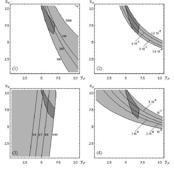
Figure 1: Results of the numerical analysis carried out for $M^{II}_{\nu 3}$ with $\epsilon=0.02$, $\epsilon^{\prime}=0.004$ and $x_{e}=y_{e}=1$. In the four frames we describe the region of the parameter space allowed by the experimental data respectively for $\Delta m^{2}_{ATM}/\Delta m^{2}_{SOL}$, $\sin^{2}2\theta_{e2}$, $\sin^{2}2\theta_{\mu 3}$ and $\tan^{2}\theta_{e3}$. The darker areas are the intersections of the allowed regions.

5 Conclusions

In this paper we have adopted the seesaw mechanism for the generation of neutrino masses. With the introduction of a right-handed neutrino for each family, the masses of the light neutrinos are given by $M_{\nu}=M_{D}M_{M}^{-1}M_{D}^{T}$, where $M_{D}$ is the Dirac mass matrix, and $M_{M}$ the Majorana mass matrix of the heavy right-handed neutrinos.

In the frame of grand-unified models, $M_{D}$ is related to the mass matrices of the quarks and charged leptons, while $M_{M}$ is completely decoupled from the charged sector. As a consequence, the matrix $M_{M}$ contains a set of arbitrary parameters, which makes these models non-predictive.

We have analysed a class of supersymmetric models based on the $SO(10)\otimes U(2)$ group, where $U(2)$ represents the flavour symmetry recently introduced [7,8] to account for the hierarchies in the mass spectrum of quarks and charged leptons. The models based on the $SO(10)$ gauge symmetry present the advantage, with respect to those based on $SU(5)$ [11], that all the unknown parameters of the Majorana mass matrix can be inglobed in a single factor.

The numerical analysis of the neutrino mass matrix shows that there is a solution, in the allowed region of the parameter space, which is consistent with the results of the three-flavour fit [13] of the existing data on solar and atmospheric neutrinos, and then in favour of the two $\nu_{e}\leftrightarrow\nu_{\mu}$ and $\nu_{\mu}\leftrightarrow\nu_{\tau}$ oscillation picture.

References

• [1] J. Ellis, Invited talk presented at the ’96 Neutrino Conference, Helsinki, 1996; preprint CERN–TH/96–325, (1996).
• [2] M. Gell–Mann, P. Ramond and R.Slansky, in Rev. Mod. Phys. 50 (1978) 721.
R.N. Mohapatra and G. Senjanovic, Phys. Rev. Let. 44 (1980) 912.
• [3] U. Amaldi, W. de Boer and H. Furstenau, Phys. Lett. B260 (1991) 447; P. Langacker and M. Luo, Phys. Rev. D44 (1991) 817.
• [4] H. Fritzsch, Phys. Lett. B70 (1977) 436; Phys. Lett. B73 (1978) 317.
• [5] P. Ramond, P. Roberts and G.G. Ross, Nucl. Phys. B406 (1993) 19.
• [6] S. Rabi, preprint OHSTPY–HEP–T–95–024 (1995);
Z. Berezhiani, preprint INFN–FE 21/95 (1995);
L.J. Hall, preprint LBL–38110/UCB–PTH–96/10 (1996).
• [7] R. Barbieri, G. Dvali and L.J. Hall, Phys. Lett. B377 (1996) 76.
• [8] A. Pomarol and D. Tommasini, preprint CERN–TH/95–207 (1995).
• [9] R. Barbieri, L.J. Hall, S. Raby and A. Romanino, preprint IFUP–TH61/96/LBL–39488 (1996).
• [10] R. Barbieri and L.J. Hall, Nuovo Cim. 100A (1997) 1.
• [11] C.D. Carone and L.J. Hall, preprint LBNL–40024/UCB–PTH–97/08 (1997).
• [12] C. Froggatt and H.B. Nielsen, Nucl. Phys. B147 (1979) 277.
• [13] G. L. Fogli, Invited talk at Les Rencontres de Physique de la Vallée d’Aoste, La Thuile (1997);
G. L. Fogli, E. Lisi and D. Montanino, 7th Intern. Workshop on Neutrino Telescopes, ed. by M. Baldo Ceolin, Venice (1996), 277, 325.