NON-PERTURBATIVE QUANTUM DYNAMICS OF A NEW INFLATION MODEL

Abstract

We consider an $O(N)$ model coupled self-consistently to gravity in the semiclassical approximation, where the field is subject to ‘new inflation’ type initial conditions. We study the dynamics self-consistently and non-perturbatively with non-equilibrium field theory methods in the large $N$ limit. We find that spinodal instabilities drive the growth of non-perturbatively large quantum fluctuations which shut off the inflationary growth of the scale factor. We find that a very specific combination of these large fluctuations plus the inflaton zero mode assemble into a new effective field. This new field behaves classically and it is the object which actually rolls down. We show how this reinterpretation saves the standard picture of how metric perturbations are generated during inflation and that the spinodal growth of fluctuations dominates the time dependence of the Bardeen variable for superhorizon modes during inflation. We compute the amplitude and index for the spectrum of scalar density and tensor perturbations and argue that in all models of this type the spinodal instabilities are responsible for a ‘red’ spectrum of primordial scalar density perturbations. A criterion for the validity of these models is provided and contact with the reconstruction program is established validating some of the results within a non-perturbative framework. The decoherence aspects and the quantum to classical transition through inflation are studied in detail by following the full evolution of the density matrix and relating the classicality of cosmological perturbations to that of long-wavelength matter fluctuations.

I Introduction and Motivation

Inflationary cosmology has come of age. From its beginnings as a solution to purely theoretical problems such as the horizon, flatness and monopole problems[1], it has grown into the main contender for the source of primordial fluctuations giving rise to large scale structure[2, 3, 4]. There is evidence from the measurements of temperature anisotropies in the cosmic microwave background radiation (CMBR) that the scale invariant power spectrum predicted by generic inflationary models is at least consistent with observations[5, 6, 7, 8, 9] and we can expect further and more exacting tests of the inflationary power spectrum when the MAP and PLANCK missions are flown. In particular, if the fluctuations that are responsible for the temperature anisotropies of the CMB truly originate from quantum fluctuations during inflation, determinations of the spectrum of scalar and tensor perturbations will constrain inflationary models based on particle physics scenarios and probably will validate or rule out specific proposals[6, 7, 10, 11]. Already current bounds on the spectrum of scalar density perturbations seem to rule out some versions of ‘extended’ inflation[10].

The tasks for inflationary universe enthusiasts are then two-fold. First, models of inflation must be constructed that have a well-defined rationale in terms of coming from a reasonable particle physics model. This is in contrast to the current situation where most, if not all acceptable inflationary models are ad-hoc in nature, with fields and potentials put in for the sole purpose of generating an inflationary epoch. Second, and equally important, we must be sure that the quantum dynamics of inflation is well understood. This is extremely important, especially in light of the fact that it is exactly this quantum behavior that is supposed to give rise to the primordial metric perturbations which presumably have imprinted themselves in the CMBR. This latter problem is the focus of this paper.

The inflaton must be treated as a non-equilibrium quantum field . The simplest way to see this comes from the requirement of having small enough metric perturbation amplitudes which in turn requires that the quartic self coupling $\lambda$ of the inflaton be extremely small, typically of order $\sim 10^{-12}$. Such a small coupling cannot establish local thermodynamic equilibrium (LTE) for all field modes; near a phase transition the long wavelength modes will respond too slowly to be able to enter LTE. In fact, the superhorizon sized modes will be out of the region of causal contact and cannot thermalize. We see then that if we want to gain a deeper understanding of inflation, non-equilibrium tools must be developed. Such tools exist and have now been developed to the point that they can give quantitative answers to these questions in cosmology[12, 13, 14, 15, 16]. These methods permit us to follow the dynamics of quantum fields in situations where the energy density is non-perturbatively large ($\sim 1/\lambda$). That is, they allow the computation of the time evolution of non-stationary states and of non-thermal density matrices.

Our approach is to apply non-equilibrium quantum field theory techniques to the situation of a scalar field coupled to semiclassical gravity, where the source of the gravitational field is the expectation value of the stress energy tensor in the relevant, dynamically changing, quantum state. In this way we can go beyond the standard analyses[17, 18, 19, 20] which treat the background as fixed.

We will mainly deal with ‘new inflation’ scenarios, where a scalar field $\phi$ evolves under the action of a typical symmetry breaking potential. The initial conditions will be taken so that the initial value of the order parameter (the field expectation value) is near the top of the potential (the disordered state) with essentially zero time derivative.

What we find is that the existence of spinodal instabilities, i.e. the fact that eventually (in an expanding universe) all modes will act as if they have a negative mass squared, drives the quantum fluctuations to grow non-perturbatively large. We have the picture of an initial wave-function or density matrix peaked near the unstable state and then spreading until it samples the stable vacua. Since these vacua are non-perturbatively far from the initial state (typically $\sim m/\sqrt{\lambda}$, where $m$ is the mass scale of the field and $\lambda$ the quartic self-coupling), the spinodal instabilities will persist until the quantum fluctuations, as encoded in the equal time two-point function $\langle\Phi(\vec{x},t)^{2}\rangle$, grow to ${\cal O}(m^{2}/\lambda$).

This growth eventually shuts off the inflationary behavior of the scale factor as well as the growth of the quantum fluctuations (this last also happens in Minkowski spacetime [12]).

The scenario envisaged here is that of a quenched or supercooled phase transition where the order parameter is zero or very small. Therefore one is led to ask:

a) What is rolling down?.

b) Since the quantum fluctuations are non-perturbatively large ( $\sim 1/\lambda$), will not they modify drastically the FRW dynamics?.

c) How can one extract (small?) metric perturbations from non-perturbatively large field fluctuations?

We address the questions a)-c) as well as other issues below.

II Non-Equilibrium Quantum Field Theory, Semiclassical Gravity and Inflation

Our program consists of finding ways to incorporate the non-equilibrium behavior of the quantum fields involved in inflation into a framework that treats gravity self consistently, at least in some approximation. We do this via the use of semiclassical gravity[21] where we say that the metric is classical, at least to first approximation, whose source is the expectation value of the stress energy tensor $\langle T_{\mu\nu}\rangle$ where this expectation value is taken in the dynamically determined state described by the density matrix $\rho(t)$. This dynamical problem can be described schematically as follows:

1. The dynamics of the scale factor $a(t)$ is driven by the semiclassical Einstein equations

   $$\frac{1}{8\pi G_{R}}G_{\mu\nu}+\frac{\Lambda_{R}}{8\pi G_{R}}g_{\mu\nu}+\left(\rm{higher\ curvature}\right)=-\langle T_{\mu\nu}\rangle_{R}.$$ (1)

   Here $G_{R},\Lambda_{R}$ are the renormalized values of Newton’s constant and the cosmological constant, respectively and $G_{\mu\nu}$ is the Einstein tensor. The higher curvature terms must be included to absorb divergences.

2. On the other hand, the density matrix $\rho(t)$ that determines $\langle T_{\mu\nu}\rangle_{R}$ obeys the Liouville equation

   $$i\frac{\partial\rho(t)}{\partial t}=\left[H,\rho(t)\right],$$ (2)

   where $H$ is the evolution Hamiltonian, which is dependent on the scale factor, $a(t)$.

It is this set of equations we must try to solve; it is clear that initial conditions must be appended to these equations for us to be able to arrive at unique solutions to them. Let us discuss some aspects of the initial state of the field theory first.

A On the initial state: dynamics of phase transitions

As we mentioned above, the situation we consider is one in which the theory admits a symmetry breaking potential and in which the field expectation value starts its evolution near the unstable point. There is an issue as to how the field got to have an expectation value near the unstable point (typically at $\Phi=0$) as well as an issue concerning the initial state of the non-zero momentum modes. The issue of initial conditions is present in any formulation of inflation but chaotic.

Since our background is an FRW spacetime, it is spatially homogeneous and we can choose our state $\rho(t)$ to respect this symmetry. Starting from the full quantum field $\Phi(\vec{x},t)$ we can extract a part that has a natural interpretation as the zero momentum, c-number part of the field by writing:

$$\Phi(\vec{x},t) = \phi(t)+\Psi(\vec{x},t)$$ (3)

$$\phi(t) = {\rm Tr}[\rho(t)\Phi(\vec{x},t)]\equiv\langle\Phi(\vec{x},t))\rangle.$$ (4)

The quantity $\Psi(\vec{x},t)$ represents the quantum fluctuations about the zero mode $\phi(t)$ and clearly satisfies $\langle\Psi(\vec{x},t)\rangle=0$.

We need to choose a basis to represent the density matrix. A natural choice consistent with the translational invariance of our quantum state is that given by the Fourier modes, in comoving momentum space, of the quantum fluctuations $\Psi(\vec{x},t)$:

$$\Psi(\vec{x},t)=\int\frac{d^{3}k}{(2\pi)^{3}}\exp(-i\ \vec{k}\cdot\vec{x})\ \psi_{k}(t).$$ (5)

In this language we can state our ansatz for the initial condition of the quantum state as follows. We take the zero mode $\phi(t=0)=\phi_{0},\ \dot{\phi}(t=0)=0$, where $\phi_{0}$ will typically be very near the origin, while the initial conditions on the the nonzero modes $\psi_{k}(t=0)$ will be chosen such that the initial density matrix $\rho(t=0)$ describes a vacuum state (i.e. an initial state in local thermal equilibrium at a temperature $T_{i}=0$). There are some subtleties involved in this choice. First, as explained in [16], in order for the density matrix to commute with the initial Hamiltonian, we must choose the modes to be initially in the conformal adiabatic vacuum (these statements will be made more precise below). This choice has the added benefit of allowing for time independent renormalization counterterms to be used in renormalizing the theory.

We are making the assumption of an initial vacuum state in order to be able to proceed with the calculation. It would be interesting to understand what forms of the density matrix can be used for other, perhaps more reasonable, initial conditions.

The assumptions of an initial equilibrium vacuum state are essentially the same used by Linde[17], Vilenkin[18] , as well as by Guth and Pi[20] in their analyses of the quantum mechanics of inflation in a fixed de Sitter background.

As discussed in the introduction, if we start from such an initial state, spinodal instabilities will drive the growth of non-perturbatively large quantum fluctuations. In order to deal with these, we need to be able to perform calculations that take these large fluctuations into account. Although the quantitative features of the dynamics will depend on the initial state, the qualitative features associated with spinodal instabilities will be fairly robust for a wide choice of initial states that describes a phase transition with a spinodal region in field space.

III The Model and Equations of Motion

Having recognized the non-perturbative dynamics of the long wavelength fluctuations, we need to study the dynamics within a non-perturbative framework. That is, a framework allowing calculations for non-perturbatively large energy densities. We require that such a framework be: i) renormalizable, ii) covariant energy conserving, iii) numerically implementable. There are very few schemes that fulfill all of these criteria: the Hartree and the large $N$ approximation[18, 12, 14]. Whereas the Hartree approximation is basically a Gaussian variational approximation[22, 23] that in general cannot be consistently improved upon, the large $N$ approximation can be consistently implemented beyond leading order[24, 25] and in our case it has the added bonus of providing many light fields (associated with Goldstone modes) that will permit the study of the effects of other fields which are lighter than the inflaton on the dynamics. Thus we will study the inflationary dynamics of a quenched phase transition within the framework of the large $N$ limit of a scalar theory in the vector representation of $O(N)$.

We assume that the universe is spatially flat with a metric given by

$$ds^{2}=dt^{2}-a^{2}(t)\,d\vec{x}^{2}\;.$$ (6)

The matter action and Lagrangian density are given by

$$S_{m}=\int d^{4}x\;{\cal L}_{m}=\int d^{4}x\;a^{3}(t)\left[\frac{1}{2}\dot{\vec{\Phi}}^{2}(x)-\frac{1}{2}\frac{(\vec{\nabla}\vec{\Phi}(x))^{2}}{a^{2}(t)}-V(\vec{\Phi}(x))\right]$$ (7)

$$V(\vec{\Phi})=\frac{\lambda}{8N}\left(\vec{\Phi}^{2}-\frac{2Nm^{2}}{\lambda}\right)^{2}+\frac{1}{2}\,\xi\;{\cal R}\;\vec{\Phi}^{2}\;,$$ (8)

$${\cal R}(t)=6\left(\frac{\ddot{a}(t)}{a(t)}+\frac{\dot{a}^{2}(t)}{a^{2}(t)}\right),$$ (9)

where we have included the coupling of $\Phi(x)$ to the scalar curvature ${\cal R}(t)$ since it will arise as a consequence of renormalization[13].

The gravitational sector includes the usual Einstein term in addition to a higher order curvature term and a cosmological constant term which are necessary to renormalize the theory. The action for the gravitational sector is therefore:

$$S_{g}=\int d^{4}x\;{\cal L}_{g}=\int d^{4}x\,a^{3}(t)\left[\frac{{\cal R}(t)}{16\pi G}+\frac{\alpha}{2}\;{\cal R}^{2}(t)-K\right].$$ (10)

with K being the cosmological constant (we use $K$ rather than the conventional $\Lambda/8\pi G$ to distinguish the cosmological constant from the ultraviolet cutoff $\Lambda$ we introduce to regularize the theory; see section IV). In principle, we also need to include the terms $R^{\mu\nu}R_{\mu\nu}$ and $R^{\alpha\beta\mu\nu}R_{\alpha\beta\mu\nu}$ as they are also terms of fourth order in derivatives of the metric (fourth adiabatic order), but the variations resulting from these terms turn out not to be independent of that of ${\cal R}^{2}$ in the flat FRW cosmology we are considering.

The variation of the action $S=S_{g}+S_{m}$ with respect to the metric $g_{\mu\nu}$ gives us Einstein’s equation

$$\frac{G_{\mu\nu}}{8\pi G}+\alpha H_{\mu\nu}+Kg_{\mu\nu}=-<T_{\mu\nu}>\;,$$ (11)

where $G_{\mu\nu}$ is the Einstein tensor given by the variation of $\sqrt{-g}{\cal R}$, $H_{\mu\nu}$ is the higher order curvature term given by the variation of $\sqrt{-g}{\cal R}^{2}$, and $T_{\mu\nu}$ is the contribution from the matter Lagrangian. With the metric (6), the various components of the curvature tensors in terms of the scale factor are:

$$G^{0}_{0} = -3(\dot{a}/a)^{2},$$ (12)

$$G^{\mu}_{\mu} = -{\cal R}=-6\left(\frac{\ddot{a}}{a}+\frac{\dot{a}^{2}}{a^{2}}\right),$$ (13)

$$H^{0}_{0} = -6\left(\frac{\dot{a}}{a}\dot{{\cal R}}+\frac{\dot{a}^{2}}{a^{2}}{\cal R}-\frac{1}{12}{\cal R}^{2}\right),$$ (14)

$$H^{\mu}_{\mu} = -6\left(\ddot{{\cal R}}+3\frac{\dot{a}}{a}\dot{{\cal R}}\right).$$ (15)

Eventually, when we have fully renormalized the theory, we will set $\alpha_{R}=0$ and keep as our only contribution to $K_{R}$ a piece related to the matter fields which we shall incorporate into $T_{\mu\nu}$.

A The Large $N$ Approximation

To obtain the proper large $N$ limit, the vector field is written as

$$\vec{\Phi}(\vec{x},t)=(\sigma(\vec{x},t),\vec{\pi}(\vec{x},t)),$$

with $\vec{\pi}$ an $(N-1)$-plet, and we write

$$\sigma(\vec{x},t)=\sqrt{N}\phi(t)+\chi(\vec{x},t)\;\;;\;\;\langle\sigma(\vec{x},t)\rangle=\sqrt{N}\phi(t)\;\;;\;\;\langle\chi(\vec{x},t)\rangle=0.$$ (16)

To implement the large $N$ limit in a consistent manner, one may introduce an auxiliary field as in[25]. However, the leading order contribution can be obtained equivalently by invoking the factorization[14, 16]:

$$\chi^{4} \rightarrow 6\langle\chi^{2}\rangle\chi^{2}+\mbox{ constant },$$ (17)

$$\chi^{3} \rightarrow 3\langle\chi^{2}\rangle\chi,$$ (18)

$$\left(\vec{\pi}\cdot\vec{\pi}\right)^{2} \rightarrow 2\langle\vec{\pi}^{2}\rangle\vec{\pi}^{2}-\langle\vec{\pi}^{2}\rangle^{2}+{\cal{O}}(1/N),$$ (19)

$$\vec{\pi}^{2}\chi^{2} \rightarrow \langle\vec{\pi}^{2}\rangle\chi^{2}+\vec{\pi}^{2}\langle\chi^{2}\rangle,$$ (20)

$$\vec{\pi}^{2}\chi \rightarrow \langle\vec{\pi}^{2}\rangle\chi.$$ (21)

To obtain a large $N$ limit, we define[14, 16]

$$\vec{\pi}(\vec{x},t)=\psi(\vec{x},t)\overbrace{\left(1,1,\cdots,1\right)}^{N-1},$$ (22)

where the large $N$ limit is implemented by the requirement that

$$\langle\psi^{2}\rangle\approx{\cal{O}}(1)\;,\;\langle\chi^{2}\rangle\approx{\cal{O}}(1)\;,\;\phi\approx{\cal{O}}(1).$$ (23)

The leading contribution is obtained by neglecting the ${\cal{O}}({1}/{N})$ terms in the formal limit. The resulting Lagrangian density is quadratic, with linear terms in $\chi$ and $\vec{\pi}$. The equations of motion are obtained by imposing the tadpole conditions $<\chi(\vec{x},t)>=0$ and $<\vec{\pi}(\vec{x},t)>=0$ which in this case are tantamount to requiring that the linear terms in $\chi$ and $\vec{\pi}$ in the Lagrangian density vanish. Since the action is quadratic, the quantum fields can be expanded in terms of creation and annihilation operators and mode functions that obey the Heisenberg equations of motion

$$\vec{\pi}(\vec{x},t)=\int\frac{d^{3}k}{(2\pi)^{3}}\left[{\vec{a}}_{k}\;f_{k}(t)\;e^{i\vec{k}\cdot\vec{x}}+{\vec{a}}^{\dagger}_{k}\;f^{*}_{k}(t)\;e^{-i\vec{k}\cdot\vec{x}}\right].$$ (24)

The tadpole condition leads to the following equations of motion[14, 16]:

$$\ddot{\phi}(t)+3H(t)\;\dot{\phi}(t)+{\cal M}^{2}(t)\;\phi(t)=0,$$ (25)

with the mode functions

$$\left[\frac{d^{2}}{dt^{2}}+3H(t)\frac{d}{dt}+\frac{k^{2}}{a^{2}(t)}+{\cal M}^{2}(t)\right]f_{k}(t)=0,$$ (26)

where

$${\cal M}^{2}(t)=-m^{2}+\xi{\cal R}+\frac{\lambda}{2}\phi^{2}(t)+\frac{\lambda}{2}\langle\psi^{2}(t)\rangle\;.$$ (27)

In this leading order in $1/N$ the theory becomes Gaussian, but with the self-consistency condition

$$\langle\psi^{2}(t)\rangle=\int\frac{d^{3}k}{(2\pi)^{3}}\frac{|f_{k}(t)|^{2}}{2}.$$ (28)

The initial conditions on the modes $f_{k}(t)$ must now be determined. At this stage it proves illuminating to pass to conformal time variables in terms of the conformally rescaled fields (see [16] and section IX for a discussion) in which the mode functions obey an equation which is very similar to that of harmonic oscillators with time dependent frequencies in Minkowski space-time. It has been realized that different initial conditions on the mode functions lead to different renormalization counterterms[16]; in particular imposing initial conditions in comoving time leads to counterterms that depend on these initial conditions. Thus we chose to impose initial conditions in conformal time in terms of the conformally rescaled mode functions leading to the following initial conditions in comoving time:

$$f_{k}(t_{0})=\frac{1}{\sqrt{W_{k}}},\;\;\;\dot{f}_{k}(t_{0})=\left[-\frac{\dot{a}(t_{0})}{a(t_{0})}-iW_{k}\right]f_{k}(t_{0}),$$ (29)

with

$$W_{k}^{2}\equiv k^{2}+{\cal M}^{2}(t_{0})-\frac{{\cal R}(t_{0})}{6}.$$ (30)

For convenience, we have set $a(t_{0})=1$ in eq. (30). At this point we recognize that when ${\cal M}^{2}(t_{0})-{\cal R}(t_{0})/6<0$ the above initial condition must be modified to avoid imaginary frequencies, which are the signal of instabilities for long wavelength modes. Thus we define the initial frequencies that determine the initial conditions (29) as

$$W_{k}^{2} \equiv k^{2}+\left|{\cal M}^{2}(t_{0})-\frac{{\cal R}(t_{0})}{6}\right|\;\mbox{ for }k^{2}<\left|{\cal M}^{2}(t_{0})-\frac{{\cal R}(t_{0})}{6}\right|\;,$$ (31)

$$W_{k}^{2} \equiv k^{2}+{\cal M}^{2}(t_{0})-\frac{{\cal R}(t_{0})}{6}\;\mbox{ for }k^{2}\geq\left|{\cal M}^{2}(t_{0})-\frac{{\cal R}(t_{0})}{6}\right|\;.$$ (32)

As an alternative we have also used initial conditions which smoothly interpolate from positive frequencies for the unstable modes to the adiabatic vacuum initial conditions defined by (29,30) for the high $k$ modes. While the alternative choices of initial conditions result in small quantitative differences in the results (a few percent in quantities which depend strongly on these low-$k$ modes), all of the qualitative features we will examine are independent of this choice.

In the large $N$ limit we find the energy density and pressure density to be given by[14, 16]

$$\frac{\varepsilon}{N} = \frac{1}{2}\dot{\phi}^{2}+\frac{1}{2}m^{2}\phi^{2}+\frac{\lambda}{8}\phi^{4}+\frac{m^{4}}{2\lambda}-\xi\;G^{0}_{0}\;\phi^{2}+6\xi\;\frac{\dot{a}}{a}\;\phi\;\dot{\phi}$$ (33)

$$+ \frac{1}{2}\langle\dot{\psi}^{2}\rangle+\frac{1}{2a^{2}}\langle(\nabla\psi)^{2}\rangle+\frac{1}{2}m^{2}\langle\psi^{2}\rangle+\frac{\lambda}{8}[2\phi^{2}\;\langle\psi^{2}\rangle+\langle\psi^{2}\rangle^{2}]$$ (34)

$$- \xi G^{0}_{0}\langle\psi^{2}\rangle+6\xi\;\frac{\dot{a}}{a}\;\langle\psi\dot{\psi}\rangle,$$ (35)

$$\frac{\varepsilon-3p}{N} = -\dot{\phi}^{2}+2m^{2}\;\phi^{2}+\frac{\lambda}{2}\;\phi^{4}+\frac{2m^{4}}{\lambda}-\xi G^{\mu}_{\mu}\phi^{2}+6\xi\left(\phi\ddot{\phi}+\dot{\phi}^{2}+3\frac{\dot{a}}{a}\phi\dot{\phi}\right)$$ (36)

$$- \langle\dot{\psi}^{2}\rangle+\frac{1}{a^{2}}\langle(\nabla\psi)^{2}\rangle+2m^{2}\;\langle\psi^{2}\rangle-\xi\;G^{\mu}_{\mu}\;\langle\psi^{2}\rangle$$ (37)

$$+ \frac{\lambda}{2}[2\phi^{2}\;\langle\psi^{2}\rangle+\langle\psi^{2}\rangle^{2}]+6\xi\left(\langle\psi\;\ddot{\psi}\rangle+\langle\dot{\psi}^{2}\rangle+3\,\frac{\dot{a}}{a}\;\langle\psi\dot{\psi}\rangle\right),$$ (38)

where $\langle\psi^{2}\rangle$ is given by equation (28) and we have defined the following integrals:

$$\langle(\nabla\psi)^{2}\rangle = \int\frac{d^{3}k}{2(2\pi)^{3}}\;k^{2}\;|f_{k}(t)|^{2}\;,$$ (39)

$$\langle\dot{\psi}^{2}\rangle = \int\frac{d^{3}k}{2(2\pi)^{3}}\;|\dot{f}_{k}(t)|^{2}\;.$$ (40)

The composite operators $\langle\psi\dot{\psi}\rangle$ and $\langle\psi\ddot{\psi}\rangle$ are symmetrized by removing a normal ordering constant to yield

$$\frac{1}{2}(\langle\psi\dot{\psi}\rangle+\langle\dot{\psi}\psi\rangle) = \frac{1}{4}\int\frac{d^{3}k}{(2\pi)^{3}}\frac{d|f_{k}(t)|^{2}}{dt}\;,$$ (41)

$$\frac{1}{2}(\langle\psi\ddot{\psi}\rangle+\langle\ddot{\psi}\psi\rangle) = \frac{1}{4}\int\frac{d^{3}k}{(2\pi)^{3}}\left[f_{k}(t)\ddot{f}_{k}^{*}(t)+\ddot{f}_{k}(t)f_{k}^{*}(t)\right]\;.$$ (42)

The last of these integrals, (42), may be rewritten using the equation of motion (26):

$$\langle\psi\ddot{\psi}\rangle=-3\frac{\dot{a}}{a}\langle\;\psi\dot{\psi}\rangle-\frac{\langle(\nabla\psi)^{2}\rangle}{a^{2}}-{\cal M}^{2}\langle\psi^{2}\rangle\;.$$ (43)

It is straightforward to show that the bare energy is covariantly conserved by using the equations of motion for the zero mode and the mode functions.

IV Renormalization

Renormalization is a very subtle but important issue in gravitational backgrounds[21]. The fluctuation contribution $\langle\psi^{2}(\vec{x},t)\rangle$, the energy, and the pressure all need to be renormalized. The renormalization aspects in curved space times have been discussed at length in the literature[21] and have been extended to the large $N$ self-consistent approximations for the non-equilibrium backreaction problem in[25, 16, 26]. More recently a consistent and covariant regularization scheme that can be implemented numerically has been provided[27].

In terms of the effective mass term for the large $N$ limit given by (27) and defining the quantity

$$B(t) \equiv a^{2}(t)\left({\cal M}^{2}(t)-{\cal{R}}/6\right),$$ (44)

$${\cal M}^{2}(t) = -m^{2}_{B}+\xi_{B}{\cal R}(t)+\frac{\lambda_{B}}{2}\phi^{2}(t)+\frac{\lambda_{B}}{2}\langle\psi^{2}(t)\rangle_{B}\;,$$ (45)

where the subscript $B$ stands for bare quantities, we find the following large $k$ behavior for the case of an arbitrary scale factor $a(t)$ (with $a(0)=1$):

$$|f_{k}(t)|^{2} = \frac{1}{ka^{2}(t)}-\frac{1}{2k^{3}a^{2}(t)}\;B(t)$$ (46)

$$+ {1\over{8k^{5}\;a^{2}(t)}}\left\{3B(t)^{2}+a(t)\frac{d}{dt}\left[a(t){\dot{B}}(t)\right]\right\}+{\cal{O}}(1/k^{7})$$ (48)

$$= {\cal S}^{(2)}+{\cal{O}}(1/k^{5})\;,$$ (50)

$$|\dot{f}_{k}(t)|^{2} = \frac{k}{a^{4}(t)}+\frac{1}{2ka^{4}(t)}\left[B(t)+2\dot{a}^{2}\right]$$ (51)

$$+ {1\over{8k^{3}\;a^{4}(t)}}\left\{-B(t)^{2}-a(t)^{2}{\ddot{B}}(t)+3a(t){\dot{a}}(t){\dot{B}}(t)-4{\dot{a}}^{2}(t)B(t)\right\}+{\cal{O}}(1/k^{5})$$ (53)

$$= {\cal S}^{(1)}+{\cal{O}}(1/k^{5})\;,$$ (55)

$$\frac{1}{2}\left[f_{k}(t)\dot{f}_{k}^{*}(t)+\dot{f}_{k}(t)f_{k}^{*}(t)\right]=-\frac{1}{k\;a^{2}(t)}\frac{\dot{a}(t)}{a(t)}-\frac{1}{4k^{3}a^{2}(t)}\left[\dot{B}(t)-2\frac{\dot{a}(t)}{a(t)}\;B(t)\right]+{\cal{O}}(1/k^{5})\;.$$ (56)

Although the divergences can be dealt with by dimensional regularization, this procedure is not well suited to numerical analysis (see however ref.[27]). We will make our subtractions using an ultraviolet cutoff, $\Lambda a(t)$, constant in physical coordinates. This guarantees that the counterterms will be time independent. The renormalization then proceeds much in the same manner as in reference[13]; the quadratic divergences renormalize the mass and the logarithmic terms renormalize the quartic coupling and the coupling to the Ricci scalar. In addition, there is a quartic divergence which renormalizes the cosmological constant while the leading renormalizations of Newton’s constant and the higher order curvature coupling are quadratic and logarithmic respectively. The renormalization conditions on the mass, coupling to the Ricci scalar and coupling constant are obtained from the requirement that the frequencies that appear in the mode equations are finite[13], i.e:

$$-m^{2}_{B}+\xi_{B}{\cal R}(t)+\frac{\lambda_{B}}{2}\phi^{2}(t)+\frac{\lambda_{B}}{2}\langle\psi^{2}(t)\rangle_{B}=-m^{2}_{R}+\xi_{R}{\cal R}(t)+\frac{\lambda_{R}}{2}\phi^{2}(t)+\frac{\lambda_{R}}{2}\langle\psi^{2}(t)\rangle_{R},$$ (57)

while the renormalizations of Newton’s constant, the higher order curvature coupling, and the cosmological constant are given by the condition of finiteness of the semi-classical Einstein-Friedmann equation:

$$\frac{G^{0}_{0}}{8\pi G_{B}}+\alpha_{B}H^{0}_{0}+K_{B}g^{0}_{0}+\langle T^{0}_{0}\rangle_{B}=\frac{G^{0}_{0}}{8\pi G_{R}}+\alpha_{R}H^{0}_{0}+K_{R}g^{0}_{0}+\langle T^{0}_{0}\rangle_{R}\;.$$ (58)

Finally we arrive at the following set of renormalizations[16]:

$$\frac{1}{8\pi NG_{R}} = \frac{1}{8\pi NG_{B}}-2\left(\xi_{R}-\frac{1}{6}\right)\frac{\Lambda^{2}}{16\pi^{2}}+2\left(\xi_{R}-\frac{1}{6}\right)m_{R}^{2}\;\frac{\ln(\Lambda/\kappa)}{16\pi^{2}},$$ (59)

$$\frac{\alpha_{R}}{N} = \frac{\alpha_{B}}{N}-\left(\xi_{R}-\frac{1}{6}\right)^{2}\frac{\ln(\Lambda/\kappa)}{16\pi^{2}},$$ (60)

$$\frac{K_{R}}{N} = \frac{K_{B}}{N}-\frac{\Lambda^{4}}{16\pi^{2}}+m_{R}^{2}\;\frac{\Lambda^{2}}{16\pi^{2}}+\frac{m_{R}^{4}}{2}\;\frac{\ln(\Lambda/\kappa)}{16\pi^{2}},$$ (61)

$$-m_{R}^{2} = -m_{B}^{2}+\lambda_{R}\;\frac{\Lambda^{2}}{16\pi^{2}}+\lambda_{R}\;m_{R}^{2}\;\frac{\ln(\Lambda/\kappa)}{16\pi^{2}},$$ (62)

$$\xi_{R} = \xi_{B}-\lambda_{R}\left(\xi_{R}-\frac{1}{6}\right)\frac{\ln(\Lambda/\kappa)}{16\pi^{2}},$$ (63)

$$\lambda_{R} = \lambda_{B}-\lambda_{R}\frac{\ln(\Lambda/\kappa)}{16\pi^{2}},$$ (64)

$$\langle\psi^{2}(t)\rangle_{R} = \int\frac{d^{3}k}{2(2\pi)^{3}}\left\{|f_{k}(t)|^{2}-\left[\frac{1}{ka^{2}(t)}-\frac{\Theta(k-\kappa)}{2k^{3}}\left[{\cal M}^{2}(t)-{{{\cal R}(t)}\over 6}\right]\right]\right\}.$$ (65)

Here, $\kappa$ is the renormalization point. As expected, the logarithmic terms are consistent with the renormalizations found using dimensional regularization[27, 26]. Again, we set $\alpha_{R}=0$ and choose the renormalized cosmological constant such that the vacuum energy is zero in the true vacuum. We emphasize that while the regulator we have chosen does not respect the covariance of the theory, the renormalized energy momentum tensor defined in this way nevertheless retains the property of covariant conservation in the limit when the cutoff is taken to infinity.

The logarithmic subtractions can be neglected because of the coupling $\lambda\leq 10^{-12}$. Using the Planck scale as the cutoff and the inflaton mass $m_{R}$ as a renormalization point, these terms are of order $\lambda\ln[M_{pl}/m_{R}]\leq 10^{-10}$, for $m\geq 10^{9}\mbox{ GeV }$. An equivalent statement is that for these values of the coupling and inflaton masses, the Landau pole is well beyond the physical cutoff $M_{pl}$. Our relative error in the numerical analysis is of order $10^{-8}$, therefore our numerical study is insensitive to the logarithmic corrections. Though these corrections are fundamentally important, numerically they can be neglected. Therefore, in the numerical computations that follow, we will neglect logarithmic renormalization and subtract only quartic and quadratic divergences in the energy and pressure, and quadratic divergences in the fluctuation contribution.

V Renormalized Equations of Motion for Dynamical Evolution

It is convenient to introduce the following dimensionless quantities and definitions,

$$\tau=m_{R}t\quad;\quad h=\frac{H}{m_{R}}\quad;\quad q=\frac{k}{m_{R}}\quad\;\quad\omega_{q}=\frac{W_{k}}{m_{R}}\quad;\quad g=\frac{\lambda_{R}}{8\pi^{2}}\;,$$ (66)

$$\eta^{2}(\tau)=\frac{\lambda_{R}}{2m^{2}_{R}}\;\phi^{2}(t)\quad;\quad g\Sigma(\tau)=\frac{\lambda}{2m^{2}_{R}}\;\langle\psi^{2}(t)\rangle_{R}\quad;\quad f_{q}(\tau)\equiv\sqrt{m_{R}}\;f_{k}(t)\;.$$ (67)

Choosing $\xi_{R}=0$ (minimal coupling) and the renormalization point $\kappa=|m_{R}|$ and setting $a(0)=1$, the equations of motion become:

$$\left[\frac{d^{2}}{d\tau^{2}}+3h\frac{d}{d\tau}-1+\eta^{2}(\tau)+g\Sigma(\tau)\right]\eta(\tau)=0,$$ (68)

$$\left[\frac{d^{2}}{d\tau^{2}}+3h\frac{d}{d\tau}+\frac{q^{2}}{a^{2}(\tau)}-1+\eta^{2}+g\Sigma(\tau)\right]f_{q}(\tau)=0,$$ (69)

$$f_{q}(0)=\frac{1}{\sqrt{\omega_{q}}}\quad;\quad\dot{f}_{q}(0)=\left[-h(0)-i\omega_{q}\right]f_{q}(0),$$ (70)

$$\omega_{q}=\left[q^{2}-1+\eta^{2}(0)-\frac{{\cal R}(0)}{6m^{2}_{R}}+g\Sigma(0)\right]^{\frac{1}{2}}\;\mbox{ for }\;q^{2}>-1+\eta^{2}(0)-\frac{{\cal R}(0)}{6m^{2}_{R}}+g\Sigma(0),$$ (71)

$$\omega_{q}=\left[q^{2}+1-\eta^{2}(0)+\frac{{\cal R}(0)}{6m^{2}_{R}}-g\Sigma(0)\right]^{\frac{1}{2}}\;\mbox{ for }\;q^{2}<-1+\eta^{2}(0)-\frac{{\cal R}(0)}{6m^{2}_{R}}+g\Sigma(0).$$ (72)

where

$$\Sigma(\tau)=\int_{0}^{\infty}q^{2}dq\left[|f_{q}(\tau)|^{2}-{1\over{a(\tau)^{2}}}+{{\Theta(q-1)}\over{2q^{3}}}\left(/frac{{\cal M}^{2}(\tau)}{m^{2}_{R}}-{{{\cal{R}(\tau)}}\over{6m^{2}_{R}}}\right)\right]\;.$$

The initial conditions for $\eta(\tau)$ will be specified later. An important point to notice is that the equation of motion for the $q=0$ mode coincides with that of the zero mode (68). Furthermore, for $\eta(\tau\rightarrow\infty)\neq 0$, a stationary (equilibrium) solution of the eq.(68) is obtained when the sum rule[12, 14, 16]

$$-1+\eta^{2}(\infty)+g\Sigma(\infty)=0$$ (73)

is fulfilled. This sum rule is nothing but a consequence of Goldstone’s theorem and is a result of the fact that the large $N$ approximation satisfies the Ward identities associated with the $O(N)$ symmetry, since the term $-1+\eta^{2}+g\Sigma$ is seen to be the effective mass of the modes transverse to the symmetry breaking direction, i.e. the Goldstone modes in the broken symmetry phase.

In terms of the zero mode $\eta(\tau)$ and the quantum mode function given by eq.(72) we find that the Friedmann equation for the dynamics of the scale factor in dimensionless variables is given by

$$h^{2}(\tau)=4h^{2}_{0}\;\epsilon_{R}(\tau)\quad;\quad h^{2}_{0}=\frac{4\pi Nm^{2}_{R}}{3M^{2}_{Pl}\lambda_{R}}$$ (74)

and the renormalized energy and pressure are given by:

$$\epsilon_{R}(\tau) = \frac{1}{2}\dot{\eta}^{2}+\frac{1}{4}\left(-1+\eta^{2}+g\Sigma\right)^{2}+$$ (76)

$$\frac{g}{2}\int q^{2}dq\left[|\dot{f_{q}}|^{2}-{\cal S}^{(1)}(q,\tau)+\frac{q^{2}}{a^{2}}\left(|f_{q}|^{2}-\Theta(q-1)\;{\cal S}^{(2)}(q,\tau)\right)\right]\;,$$

$$(p+\varepsilon)_{R}(\tau) = \frac{2Nm^{4}_{R}}{\lambda_{R}}\left\{\dot{\eta}^{2}\right.$$ (77)

$$+ \left.g\int q^{2}dq\left[|\dot{f_{q}}|^{2}-{\cal S}^{(1)}(q,\tau)+\frac{q^{2}}{3a^{2}}\left(|f_{q}|^{2}-\Theta(q-1)\;{\cal S}^{(2)}(q,\tau)\right)\right]\right\},$$ (78)

where the subtractions ${\cal S}^{(1)}$ and ${\cal S}^{(2)}$ are given by the right hand sides of eqns.(55) and (50) respectively.

The renormalized energy and pressure are covariantly conserved:

$${\dot{\epsilon}}_{R}(\tau)+3\,h(\tau)\,(p+\varepsilon)_{R}(\tau)=0\;.$$ (79)

In order to provide the full solution we now must provide the values of $\eta(0)$, $\dot{\eta}(0)$, and $h_{0}$. Assuming that the inflationary epoch is associated with a phase transition at the GUT scale, this requires that $Nm^{4}_{R}/\lambda_{R}\approx(10^{15}\mbox{ Gev })^{4}$ and assuming the bound on the scalar self-coupling $\lambda_{R}\approx 10^{-12}-10^{-14}$ (this will be seen later to be a compatible requirement), we find that $h_{0}\approx N^{1/4}$ which we will take to be reasonably given by $h_{0}\approx 1-10$ (for example in popular GUT’s $N\approx 20$ depending on particular representations).

We will begin by studying the case of most interest from the point of view of describing the phase transition: $\eta(0)=0$ and $\dot{\eta}(0)=0$, which are the initial conditions that led to puzzling questions. With these initial conditions, the evolution equation for the zero mode eq.(68) determines that $\eta(\tau)=0$ by symmetry.

A Early time dynamics:

Before engaging in the numerical study, it proves illuminating to obtain an estimate of the relevant time scales and an intuitive idea of the main features of the dynamics. Because the coupling is so weak ($g\sim 10^{-12}\ll 1$) and after renormalization the contribution from the quantum fluctuations to the equations of motion is finite, we can neglect all the terms proportional to $g$ in eqs.(76) and (72).

For the case where we choose $\eta(\tau)=0$ and the evolution equations for the mode functions are those for an inverted oscillator in De Sitter space-time, which have been studied by Guth and Pi[20]. One obtains the approximate solution

$$h(t) \approx h_{0},$$ (80)

$$f_{q}(t) \approx e^{-3h_{0}\tau/2}\left[A_{q}\;J_{\nu}\left(\frac{q}{h_{0}}e^{-h_{0}\tau}\right)+B_{q}\;J_{-\nu}\left(\frac{q}{h_{0}}e^{-h_{0}\tau}\right)\right],$$ (81)

$$\nu = \sqrt{\frac{9}{4}+\frac{1}{h^{2}_{0}}},$$ (82)

where $J_{\pm\nu}(z)$ are Bessel functions, and $A_{q}$ and $B_{q}$ are determined by the initial conditions on the mode functions:

$$B_{q}=-\frac{1}{\sqrt{\omega_{q}}}{{\pi\,q}\over{2h_{0}\,\sin{\nu\pi}}}\;\left[{{i\omega_{q}-\frac{1}{2}\,h_{0}}\over q}\;J_{\nu}\left(\frac{q}{h_{0}}\right)-J^{\prime}_{\nu}\left(\frac{q}{h_{0}}\right)\right],$$ (83)

$$A_{q}=\frac{1}{\sqrt{\omega_{q}}}{{\pi\,q}\over{2h_{0}\,\sin{\nu\pi}}}\;\left[{{i\omega_{q}-\frac{1}{2}\,h_{0}}\over q}\;J_{-\nu}\left(\frac{q}{h_{0}}\right)-J^{\prime}_{-\nu}\left(\frac{q}{h_{0}}\right)\right]\;.$$ (84)

After the physical wavevectors cross the horizon, i.e. when $qe^{-h_{0}\tau}/h_{0}\ll 1$ we find that the mode functions factorize:

$$f_{q}(\tau)\approx{{B_{q}}\over{\Gamma(1-\nu)}}\;\left({{2h_{0}\,}\over q}\right)^{\nu}e^{(\nu-3/2)h_{0}\tau}.$$ (85)

This result reveals a very important feature: because of the negative mass squared term in the matter Lagrangian leading to symmetry breaking (and $\nu>3/2$), we see that all of the mode functions grow exponentially after horizon crossing (for positive mass squared $\nu<3/2$, and they would decrease exponentially after horizon crossing). This exponential growth is a consequence of the spinodal instabilities which is a hallmark of the process of phase separation that occurs to complete the phase transition. We note, in addition that the time dependence is exactly given by that of the $q=0$ mode, i.e. the zero mode, which is a consequence of the redshifting of the wavevectors and the fact that after horizon crossing the contribution of the term $q^{2}/a^{2}(\tau)$ in the equations of motion become negligible. We clearly see that the quantum fluctuations grow exponentially and they will begin to be of the order of the tree level terms in the equations of motion when $g\Sigma(\tau)\approx 1$. At large times

$$\Sigma(\tau)\approx{\cal F}^{2}(h_{0})h_{0}^{2}e^{(2\nu-3)h_{0}\tau}\;,$$

with ${\cal F}(h_{0})$ a finite constant that depends on the initial conditions and is found numerically to be of ${\cal O}(1)$ [see figure (10)].

In terms of the initial dimensionful variables, the condition $g\Sigma(\tau)\approx 1$ translates to $<\psi^{2}(\vec{x},t)>_{R}\approx 2m^{2}_{R}/\lambda_{R}$, i.e. the quantum fluctuations sample the minima of the (renormalized) tree level potential. We find that the time at which the contribution of the quantum fluctuations becomes of the same order as the tree level terms is estimated to be[14]

$$\tau_{s}\approx\frac{1}{(2\nu-3)h_{0}}\ln\left[\frac{1}{g\,h_{0}^{2}{\cal F}^{2}(h_{0})}\right]=\frac{3}{2}h_{0}\ln\left[\frac{1}{g\,h_{0}^{2}{\cal F}^{2}(h_{0})}\right]+{\cal O}(1/h_{0}).$$ (86)

At this time, the contribution of the quantum fluctuations makes the back reaction very important and, as will be seen numerically, this translates into the fact that $\tau_{s}$ also determines the end of the De Sitter era and the end of inflation. The total number of e-folds during the stage of exponential expansion of the scale factor (constant $h_{0}$) is given by

$$N_{e}\approx\frac{1}{2\nu-3}\;\ln\left[\frac{1}{g\;h_{0}^{2}\;{\cal F}^{2}(h_{0})}\right]=\frac{3}{2}\;h_{0}^{2}\;\ln\left[\frac{1}{g\;h_{0}^{2}\;{\cal F}^{2}(h_{0})}\right]+{\cal O}(1)$$ (87)

For large $h_{0}$ we see that the number of e-folds scales as $h^{2}_{0}$ as well as with the logarithm of the inverse coupling. These results (85,86,87) will be confirmed numerically below and will be of paramount importance for the interpretation of the main consequences of the dynamical evolution.

B $\eta(0)\neq 0$: classical or quantum behavior?

Above we have analyzed the situation when $\eta(0)=0$ (or in dimensionful variables $\phi(0)=0$). The typical analysis of inflaton dynamics in the literature involves the classical evolution of $\phi(t)$ with an initial condition in which $\phi(0)$ is very close to zero (i.e. the top of the potential hill) in the ‘slow-roll’ regime, for which $\ddot{\phi}\ll 3H\dot{\phi}$. Thus, it is important to quantify the initial conditions on $\phi(t)$ for which the dynamics will be determined by the classical evolution of $\phi(t)$ and those for which the quantum fluctuations dominate the dynamics. We can provide a criterion to separate classical from quantum dynamics by analyzing the relevant time scales, estimated by neglecting non-linearities and backreaction effects. We consider the evolution of the zero mode in terms of dimensionless variables, and choose $\eta(0)\neq 0$ and $\dot{\eta}(0)=0$. ($\dot{\eta}(0)\neq 0$ simply corresponds to a shift in origin of time). We assume $\eta(0)^{2}<<1$ which is the relevant case where spinodal instabilities are important. We find

$$\eta(\tau)\approx\eta(0)\;e^{(\nu-\frac{3}{2})h_{0}\tau}\;.$$ (88)

The non-linearities will become important and eventually terminate inflation when $\eta(\tau)\approx 1$. This corresponds to a time scale given by

$$\tau_{c}\approx\frac{\ln\left[1/\eta(0)\right]}{(\nu-\frac{3}{2})\;h_{0}}\;.$$ (89)

If $\tau_{c}$ is much smaller than the spinodal time $\tau_{s}$ given by eq.(86) then the classical evolution of the zero mode will dominate the dynamics and the quantum fluctuations will not become very large, although they will still undergo spinodal growth. On the other hand, if $\tau_{c}\gg\tau_{s}$ the quantum fluctuations will grow to be very large well before the zero mode reaches the non-linear regime. In this case the dynamics will be determined completely by the quantum fluctuations. Then the criterion for the classical or quantum dynamics is given by

$$\eta(0) \gg \sqrt{g}\;h_{0}\Longrightarrow\mbox{ classical dynamics }$$ (90)

$$\eta(0) \ll \sqrt{g}\;h_{0}\Longrightarrow\mbox{ quantum dynamics }$$ (91)

or in terms of dimensionful variables $\phi(0)\gg H_{0}$ leads to classical dynamics and $\phi(0)\ll H_{0}$ leads to quantum dynamics.

However, even when the classical evolution of the zero mode dominates the dynamics, the quantum fluctuations grow exponentially after horizon crossing unless the value of $\phi(t)$ is very close to the minimum of the tree level potential. In the large $N$ approximation the spinodal line, that is the values of $\phi(t)$ for which there are spinodal instabilities, reaches all the way to the minimum of the tree level potential as can be seen from the equations of motion for the mode functions. Therefore even in the classical case one must understand how to deal with quantum fluctuations that grow after horizon crossing.

C Numerics

The time evolution is carried out by means of a fourth order Runge-Kutta routine with adaptive stepsizing while the momentum integrals are carried out using an 11-point Newton-Cotes integrator. The relative errors in both the differential equation and the integration are of order $10^{-8}$. We find that the energy is covariantly conserved throughout the evolution to better than a part in a thousand. Figures (1–3) show $g\Sigma(\tau)$ vs. $\tau$, $h(\tau)$ vs. $\tau$ and $\ln(|f_{q}(\tau)|^{2})$ vs. $\tau$ for several values of $q$ with larger $q^{\prime}s$ corresponding to successively lower curves. Figures (4,5) show $p(\tau)/\varepsilon(\tau)$ and the horizon size $h^{-1}(\tau)$ for $g=10^{-14}\;;\;\eta(0)=0\;;\;\dot{\eta}(0)=0$ and we have chosen the representative value $h_{0}=2.0$.

Figures (1) and (2) show clearly that when the contribution of the quantum fluctuations $g\Sigma(\tau)$ becomes of order 1 inflation ends, and the time scale for $g\Sigma(\tau)$ to reach ${\cal O}(1)$ is very well described by the estimate (86). From figure 1 we see that this happens for $\tau=\tau_{s}\approx 90$, leading to a number of e-folds $N_{e}\approx 180$ which is correctly estimated by (86, 87).

Figure (3) shows clearly the factorization of the modes after they cross the horizon as described by eq.(85). The slopes of all the curves after they become straight lines in figure (3) is given exactly by $(2\nu-3)$, whereas the intercept depends on the initial condition on the mode function and the larger the value of $q$ the smaller the intercept because the amplitude of the mode function is smaller initially. Although the intercept depends on the initial conditions on the long-wavelength modes, the slope is independent of the value of $q$ and is the same as what would be obtained in the linear approximation for the square of the zero mode at times long enough that the decaying solution can be neglected but short enough that the effect of the non-linearities is very small. Notice from the figure that when inflation ends and the non-linearities become important all of the modes effectively saturate. This is also what one would expect from the solution of the zero mode: exponential growth in early-intermediate times (neglecting the decaying solution), with a growth exponent given by $(\nu-3/2)$ and an asymptotic behavior of small oscillations around the equilibrium position, which for the zero mode is $\eta=1$, but for the $q\neq 0$ modes depends on the initial conditions. All of the mode functions have this behavior once they cross the horizon. We have also studied the phases of the mode functions and we found that they freeze after horizon crossing in the sense that they become independent of time. This is natural since both the real and imaginary parts of $f_{q}(\tau)$ obey the same equation but with different boundary conditions. After the physical wavelength crosses the horizon, the dynamics is insensitive to the value of $q$ for real and imaginary parts and the phases become independent of time. Again, this is a consequence of the factorization of the modes.

The growth of the quantum fluctuations is sufficient to end inflation at a time given by $\tau_{s}$ in eq.(86). Furthermore figure (4) shows that during the inflationary epoch $p(\tau)/\varepsilon(\tau)\approx-1$ and the end of inflation is rather sharp at $\tau_{s}$ with $p(\tau)/\varepsilon(\tau)$ oscillating between $\pm 1$ with zero average over the cycles, resulting in matter domination. Figure (5) shows this feature very clearly; $h(\tau)$ is constant during the De Sitter epoch and becomes matter dominated after the end of inflation with $h^{-1}(\tau)\approx\frac{3}{2}(\tau-\tau_{s})$. There are small oscillations around this value because both $p(\tau)$ and $\varepsilon(\tau)$ oscillate. These oscillations are a result of small oscillations of the mode functions after they saturate, and are also a feature of the solution for a zero mode.

All of these features hold for a variety of initial conditions. As an example, we show in figures (6) – (9) the plots corresponding to figs. (1) – (4) for the case of an initial Hubble parameter of $h_{0}=10$.

D Zero Mode Assembly:

This remarkable feature of factorization of the mode functions after horizon crossing can be elegantly summarized as

$$f_{k}(t)|_{k_{ph}(t)\ll H_{0}}=g(q,h_{0})f_{0}(\tau),$$ (92)

with $k_{ph}(t)=k\,e^{-H_{0}t}$ being the physical momentum, $g(q,h_{0})$ a complex constant, and $f_{0}(\tau)$ a real function of time that satisfies the mode equation with $q=0$ and real initial conditions which will be inferred later. Since the factor $g(q,h_{0})$ depends solely on the initial conditions on the mode functions, it turns out that for two mode functions corresponding to momenta $k_{1},k_{2}$ that have crossed the horizon at times $t_{1}>t_{2}$, the ratio of the two mode functions at time $t$, ($t_{s}>t>t_{1}>t_{2}$) is

$${{f_{k_{1}}(t)}\over{f_{k_{2}}(t)}}\propto e^{(\nu-\frac{3}{2})h_{0}(\tau_{1}-\tau_{2})}>1\;.$$

Then if we consider the contribution of these modes to the renormalized quantum fluctuations a long time after the beginning of inflation (so as to neglect the decaying solutions), we find that

$$g\Sigma(\tau)\approx{\cal C}e^{(2\nu-3)h_{0}\tau}+\mbox{ small}\;,$$

where ‘small’ stands for the contribution of mode functions associated with momenta that have not yet crossed the horizon at time $\tau$, which give a perturbatively small (of order $\lambda$) contribution. We find that several e-folds after the beginning of inflation but well before inflation ends, this factorization of superhorizon modes implies the following:

$$g\int q^{2}dq\;|f^{2}_{q}(\tau)| \approx |C_{0}|^{2}f^{2}_{0}(\tau),$$ (93)

$$g\int q^{2}dq\;|\dot{f}^{2}_{q}(\tau)| \approx |C_{0}|^{2}\dot{f}^{2}_{0}(\tau),$$ (94)

$$g\int\frac{q^{4}}{a^{2}(\tau)}dq\;|f^{2}_{q}(\tau)| \approx \frac{|C_{1}|^{2}}{a^{2}(\tau)}f^{2}_{0}(\tau),$$ (95)

where we have neglected the weak time dependence arising from the perturbatively small contributions of the short-wavelength modes that have not yet crossed the horizon, and the integrals above are to be understood as the fully renormalized (subtracted), finite integrals. For $\eta=0$, we note that (93) and the fact that $f_{0}(\tau)$ obeys the equation of motion for the mode with $q=0$ leads at once to the conclusion that in this regime $\left[g\Sigma(\tau)\right]^{\frac{1}{2}}=|C_{0}|f_{0}(\tau)$ obeys the zero mode equation of motion

$$\left[\frac{d^{2}}{d\tau^{2}}+3h\frac{d}{d\tau}-1+(|C_{0}|f_{0}(\tau))^{2}\right]|C_{0}|f_{0}(\tau)=0\;.$$ (96)

It is clear that several e-folds after the beginning of inflation, we can define an effective zero mode as

$$\eta^{2}_{eff}(\tau)\equiv g\Sigma(\tau),\mbox{ or in dimensionful variables, }\phi_{eff}(t)\equiv\left[\langle\psi^{2}(\vec{x},t)\rangle_{R}\right]^{\frac{1}{2}}$$ (97)

Although this identification seems natural, we emphasize that it is by no means a trivial or ad-hoc statement. There are several important features that allow an unambiguous identification: i) $\left[\langle\psi^{2}(\vec{x},t)\rangle_{R}\right]$ is a fully renormalized operator product and hence finite, ii) because of the factorization of the superhorizon modes that enter in the evaluation of $\left[\langle\psi^{2}(\vec{x},t)\rangle_{R}\right]$, $\phi_{eff}(t)$ (97) obeys the equation of motion for the zero mode, iii) this identification is valid several e-folds after the beginning of inflation, after the transient decaying solutions have died away and the integral in $\langle\psi^{2}(\vec{x},t)\rangle$ is dominated by the modes with wavevector $k$ that have crossed the horizon at $t(k)\ll t$. Numerically we see that this identification holds throughout the dynamics except for a very few e-folds at the beginning of inflation. This factorization determines at once the initial conditions of the effective zero mode that can be extracted numerically: after the first few e-folds and long before the end of inflation we find

$$\phi_{eff}(t)\equiv\phi_{eff}(0)\;e^{(\nu-\frac{3}{2})H_{0}t}\;\;,$$ (98)

where we parameterized

$$\phi_{eff}(0)\equiv\frac{H_{0}}{2\pi}\;{\cal F}(H_{0}/m)$$

to make contact with the literature. As is shown in fig. (10), we find numerically that ${\cal F}(H_{0}/m)\approx{\cal O}(1)$ for a large range of $0.1\leq H_{0}/m\leq 50$ and that this quantity depends on the initial conditions of the long wavelength modes.

Therefore, in summary, the effective composite zero mode obeys

$$\left[\frac{d^{2}}{d\tau^{2}}+3h\frac{d}{d\tau}-1+\eta^{2}_{eff}(\tau)\right]\eta_{eff}(\tau)=0\;;\;\dot{\eta}_{eff}(\tau=0)=(\nu-\frac{3}{2})\;\eta_{eff}(0)\;,$$ (99)

where $\eta_{eff}(0)\equiv{{\sqrt{\lambda_{R}/2}}\over{m_{R}}}\;\phi_{eff}(0)$ is obtained numerically for a given $h_{0}$ by fitting the intermediate time behavior of $g\Sigma(\tau)$ with the growing zero mode solution.

Furthermore, this analysis shows that in the case $\eta=0$, the renormalized energy and pressure in this regime in which the renormalized integrals are dominated by the superhorizon modes are given by

$$\varepsilon_{R}(\tau) \approx \frac{2Nm^{4}_{R}}{\lambda_{R}}\left\{\frac{1}{2}\dot{\eta}^{2}_{eff}+\frac{1}{4}\left(-1+\eta^{2}_{eff}\right)^{2}\right\},$$ (100)

$$(p+\varepsilon)_{R} \approx \frac{2Nm^{4}_{R}}{\lambda_{R}}\left\{\dot{\eta}^{2}_{eff}\right\},$$ (101)

where we have neglected the contribution proportional to $1/a^{2}(\tau)$ because it is effectively red-shifted away after just a few e-folds. We found numerically that this term is negligible after the interval of time necessary for the superhorizon modes to dominate the contribution to the integrals. Then the dynamics of the scale factor is given by

$$h^{2}(\tau)=4h^{2}_{0}\left\{\frac{1}{2}\dot{\eta}^{2}_{eff}+\frac{1}{4}\left(-1+\eta^{2}_{eff}\right)^{2}\right\}.$$ (102)

We have numerically evolved the set of effective equations (99, 102) by extracting the initial condition for the effective zero mode from the intermediate time behavior of $g\Sigma(\tau)$. We found a remarkable agreement between the evolution of $\eta^{2}_{eff}$ and $g\Sigma(\tau)$ and between the dynamics of the scale factor in terms of the evolution of $\eta_{eff}(\tau)$, and the full dynamics of the scale factor and quantum fluctuations within our numerical accuracy. Figures (11) and (12) show the evolution of $\eta^{2}_{eff}(\tau)$ and $h(\tau)$ respectively from the classical evolution equations (99) and (102) using the initial condition $\eta_{eff}(0)$ extracted from the exponential fit of $g\Sigma(\tau)$ in the intermediate regime. These figures should be compared to Figure (1) and (2). We have also numerically compared $p/\varepsilon$ given solely by the dynamics of the effective zero mode and it is again numerically indistinguishable from that obtained with the full evolution of the mode functions.

This is one of the main results of our work. In summary: the modes that become superhorizon sized and grow through the spinodal instabilities assemble themselves into an effective composite zero mode a few e-folds after the beginning of inflation. This effective zero mode drives the dynamics of the FRW scale factor, terminating inflation when the non-linearities become important. In terms of the underlying fluctuations, the spinodal growth of superhorizon modes gives a non-perturbatively large contribution to the energy momentum tensor that drives the dynamics of the scale factor. Inflation terminates when the mean square root fluctuation probes the equilibrium minima of the tree level potential.

This phenomenon of zero mode assembly, i.e. the ‘classicalization’ of quantum mechanical fluctuations that grow after horizon crossing is very similar to the interpretation of ‘decoherence without decoherence’ of Starobinsky and Polarski[28].

The extension of this analysis to the case for which $\eta(0)\neq 0$ is straightforward. Since both $\eta(\tau)$ and $\sqrt{g\Sigma(\tau)}=|C_{0}|f_{0}(\tau)$ obey the equation for the zero mode, eq.(68), it is clear that we can generalize our definition of the effective zero mode to be

$$\eta_{eff}(\tau)\equiv\sqrt{\eta^{2}(\tau)+g\Sigma(\tau)}\;.$$ (103)

which obeys the equation of motion of a classical zero mode:

$$\left[\frac{d^{2}}{d\tau^{2}}+3h\frac{d}{d\tau}-1+\eta_{eff}(\tau)^{2}\right]\eta_{eff}(\tau)=0\;.$$ (104)

If this effective zero mode is to drive the FRW expansion, then the additional condition

$$\dot{\eta}^{2}f_{0}^{2}-2\eta\dot{\eta}f_{0}\dot{f_{0}}+\eta^{2}\dot{f_{0}}^{2}=0$$ (105)

must also be satisfied. One can easily show that this relation is indeed satisfied if the mode functions factorize as in (92) and if the integrals (93) – (95) are dominated by the contributions of the superhorizon mode functions. This leads to the conclusion that the gravitational dynamics is given by eqns. (100) – (102) with $\eta_{eff}(\tau)$ defined by (103).

We see that in all cases, the full large $N$ quantum dynamics in these models of inflationary phase transitions is well approximated by the equivalent dynamics of a homogeneous, classical scalar field with initial conditions on the effective field $\eta_{eff}(0)\geq\sqrt{g}h_{0}{\cal F}(h_{0})$. We have verified these results numerically for the field and scale factor dynamics, finding that the effective classical dynamics reproduces the results of the full dynamics to within our numerical accuracy. We have also checked numerically that the estimate for the classical to quantum crossover given by eq.(91) is quantitatively correct. Thus in the classical case in which $\eta(0)\gg\sqrt{\lambda}\;h_{0}$ we find that $\eta_{eff}(\tau)=\eta(\tau)$, whereas in the opposite, quantum case $\eta_{eff}(\tau)=\sqrt{g\Sigma(\tau)}$.

This remarkable feature of zero mode assembly of long-wavelength, spinodally unstable modes is a consequence of the presence of the horizon. It also explains why, despite the fact that asymptotically the fluctuations sample the broken symmetry state, the equation of state is that of matter. Since the excitations in the broken symmetry state are massless Goldstone bosons one would expect radiation domination. However, the assembly phenomenon, i.e. the redshifting of the wave vectors, makes these modes behave exactly like zero momentum modes that give an equation of state of matter (upon averaging over the small oscillations around the minimum).

Subhorizon modes at the end of inflation with $q>h_{0}\,e^{h_{0}\tau_{s}}$ do not participate in the zero mode assembly. The behavior of such modes do depend on $q$ after the end of inflation. Notice that these modes have extremely large comoving $q$ since $h_{0}\,e^{h_{0}\tau_{s}}\geq 10^{26}$. As discussed in ref.[16] such modes decrease with time after inflation as $\sim 1/a(\tau)$.

VI Making sense of small fluctuations:

Having recognized the effective classical variable that can be interpreted as the component of the field that drives the FRW background and rolls down the classical potential hill, we want to recognize unambiguously the small fluctuations. We have argued above that after horizon crossing, all of the mode functions evolve proportionally to the zero mode, and the question arises: which modes are assembled into the effective zero mode whose dynamics drives the evolution of the FRW scale factor and which modes are treated as perturbations? In principle every $k\neq 0$ mode provides some spatial inhomogeneity, and assembling these into an effective homogeneous zero mode seems in principle to do away with the very inhomogeneities that one wants to study. However, scales of cosmological importance today first crossed the horizon during the last 60 or so e-folds of inflation. Recently Grishchuk[29] has argued that the sensitivity of the measurements of $\Delta T/T$ probe inhomogeneities on scales $\approx 500$ times the size of the present horizon. Therefore scales that are larger than these and that have first crossed the horizon much earlier than the last 60 e-folds of inflation are unobservable today and can be treated as an effective homogeneous component, whereas the scales that can be probed experimentally via the CMB inhomogeneities today must be treated separately as part of the inhomogeneous perturbations of the CMB.

Thus a consistent description of the dynamics in terms of an effective zero mode plus ‘small’ quantum fluctuations can be given provided the following requirements are met: a) the total number of e-folds $N_{e}\gg 60$, b) all the modes that have crossed the horizon before the last 60-65 e-folds are assembled into an effective classical zero mode via $\phi_{eff}(t)=\left[\phi^{2}_{0}(t)+\langle\psi^{2}(\vec{x},t)\rangle_{R}\right]^{\frac{1}{2}}$, c) the modes that cross the horizon during the last 60–65 e-folds are accounted as ‘small’ perturbations. The reason for the requirement a) is that in the separation $\phi(\vec{x},t)=\phi_{eff}(t)+\delta\phi(\vec{x},t)$ one requires that $\delta\phi(\vec{x},t)/\phi_{eff}(t)\ll 1$. As argued above, after the modes cross the horizon, the ratio of amplitudes of the mode functions remains constant and given by $e^{(\nu-\frac{3}{2})\Delta N}$ with $\Delta N$ being the number of e-folds between the crossing of the smaller $k$ and the crossing of the larger $k$. Then for $\delta\phi(\vec{x},t)$ to be much smaller than the effective zero mode, it must be that the Fourier components of $\delta\phi$ correspond to very large $k$’s at the beginning of inflation, so that the effective zero mode can grow for a long time before the components of $\delta\phi$ begin to grow under the spinodal instabilities. In fact requirement a) is not very severe; in the figures (1-5) we have taken $h_{0}=2.0$ which is a very moderate value and yet for $\lambda=10^{-12}$ the inflationary stage lasts for well over 100 e-folds, and as argued above, the larger $h_{0}$ for fixed $\lambda$, the longer is the inflationary stage. Therefore under this set of conditions, the classical dynamics of the effective zero mode $\phi_{eff}(t)$ drives the FRW background, whereas the inhomogeneous fluctuations $\delta\phi(\vec{x},t)$, which are made up of Fourier components with wavelengths that are much smaller than the horizon at the beginning of inflation and that cross the horizon during the last 60 e-folds, provide the inhomogeneities that seed density perturbations.

VII Scalar and Tensor Metric Perturbations:

A Scalar Perturbations:

Having identified the effective zero mode and the ‘small perturbations’, we are now in position to provide an estimate for the amplitude and spectrum of scalar metric perturbations. We use the clear formulation by Mukhanov, Feldman and Brandenberger[30] in terms of gauge invariant variables. In particular we focus on the dynamics of the Bardeen potential[31], which in longitudinal gauge is identified with the Newtonian potential. The equation of motion for the Fourier components (in terms of comoving wavevectors) for this variable in terms of the effective zero mode is[30]

$$\ddot{\Phi}_{k}+\left[H(t)-2\frac{\ddot{\phi}_{eff}(t)}{\dot{\phi}_{eff}(t)}\right]\dot{\Phi}_{k}+\left[\frac{k^{2}}{a^{2}(t)}+2\left(\dot{H}(t)-H(t)\frac{\ddot{\phi}_{eff}(t)}{\dot{\phi}_{eff}(t)}\right)\right]\Phi_{k}=0.$$ (106)

We are interested in determining the dynamics of $\Phi_{k}$ for those wavevectors that cross the horizon during the last 60 e-folds before the end of inflation. During the inflationary stage the numerical analysis yields to a very good approximation

$$H(t)\approx H_{0}\;;\;\phi_{eff}(t)=\phi_{eff}(0)\;e^{(\nu-\frac{3}{2})H_{0}t},$$ (107)

where $H_{0}$ is the value of the Hubble constant during inflation, leading to

$$\Phi_{k}(t)=e^{(\nu-2)H_{0}t}\left[a_{k}\;H^{(1)}_{\beta}\left(\frac{ke^{-H_{0}t}}{H_{0}}\right)+b_{k}\;H^{(2)}_{\beta}\left(\frac{ke^{-H_{0}t}}{H_{0}}\right)\right]\;;\;\beta=\nu-1\;.$$ (108)

The coefficients $a_{k},b_{k}$ are determined by the initial conditions.

Since we are interested in the wavevectors that cross the horizon during the last 60 e-folds, the consistency for the zero mode assembly and the interpretation of ‘small perturbations’ requires that there must be many e-folds before the last 60. We are then considering wavevectors that were deep inside the horizon at the onset of inflation. Mukhanov et. al.[30] show that $\Phi_{k}(t)$ is related to the canonical ‘velocity field’ that determines scalar perturbations of the metric and which is quantized with Bunch-Davies initial conditions for the large $k$-mode functions. The relation between $\Phi_{k}$ and $v$ and the initial conditions on $v$ lead at once to a determination of the coefficients $a_{k}$ and $b_{k}$ for $k>>H_{0}$[30]

$$a_{k}=-\frac{3}{2}\left[\frac{8\pi}{3M^{2}_{Pl}}\right]\dot{\phi}_{eff}(0)\sqrt{\frac{\pi}{2H_{0}}}\frac{1}{k}\quad;\quad b_{k}=0\;.$$ (109)

Thus we find that the amplitude of scalar metric perturbations after horizon crossing is given by

$$|\delta_{k}(t)|=k^{\frac{3}{2}}|\Phi_{k}(t)|\approx\frac{3}{2}\left[\frac{8\sqrt{\pi}}{3M^{2}_{Pl}}\right]\dot{\phi}_{eff}(0)\left(\frac{2H_{0}}{k}\right)^{\nu-\frac{3}{2}}e^{(2\nu-3)H_{0}t}\;.$$ (110)

The power spectrum per logarithmic $k$ interval is given by $|\delta_{k}(t)|^{2}$. The time dependence of $|\delta_{k}(t)|$ displays the unstable growth associated with the spinodal instabilities of super-horizon modes and is a hallmark of the phase transition. This time dependence can be also understood from the constraint equation that relates the Bardeen potential to the gauge invariant field fluctuations[30], which in longitudinal gauge are identified with $\delta\phi(\vec{x},t)$. The constraint equation and the evolution equations for the gauge invariant scalar field fluctuations are[30]

$$\frac{d}{dt}(a\Phi_{k})=\frac{4\pi}{M^{2}_{Pl}}\;a\;\delta\phi^{gi}_{k}\;\dot{\phi}_{0}\;,$$ (111)

$$\left[\frac{d^{2}}{dt^{2}}+3H\frac{d}{dt}+\frac{k^{2}}{a^{2}}+{\cal M}^{2}\right]\delta\phi^{gi}_{k}-4\;\dot{\phi}_{eff}\;\dot{\Phi}_{k}+2V^{\prime}(\phi_{eff})\;\Phi_{k}=0\;.$$ (112)

Since the right hand side of (111) is proportional to $\dot{\phi}_{eff}/M^{2}_{Pl}\ll 1$ during the inflationary epoch in this model, we can neglect the terms proportional to $\dot{\Phi}_{k}$ and $\Phi_{k}$ on the left hand side of (112), in which case the equation for the gauge invariant scalar field fluctuation is the same as for the mode functions. In fact, since $\delta\phi^{gi}_{k}$ is gauge invariant we can evaluate it in the longitudinal gauge wherein it is identified with the mode functions $f_{k}(t)$. Then absorbing a constant of integration in the initial conditions for the Bardeen variable, we find

$$\Phi_{k}(t)\approx\frac{4\pi}{M^{2}_{Pl}a(t)}\int_{t_{o}}^{t}a(t^{\prime})\;\phi_{eff}(t^{\prime})\;f_{k}(t^{\prime})\;dt^{\prime}+{\cal O}\left(\frac{1}{M^{4}_{Pl}}\right),$$ (113)

and using that $\phi(t)\propto e^{(\nu-3/2)H_{0}t}$ and that after horizon crossing $f_{k}(t)\propto e^{(\nu-3/2)H_{0}t}$, one obtains at once the time dependence of the Bardeen variable after horizon crossing. In particular the time dependence is found to be $\propto e^{(2\nu-3)H_{0}t}$. It is then clear that the time dependence is a reflection of the spinodal (unstable) growth of the superhorizon field fluctuations.

To obtain the amplitude and spectrum of density perturbations at second horizon crossing we use the conservation law associated with the gauge invariant variable[30]

$$\xi_{k}=\frac{2}{3}\frac{\frac{\dot{\Phi}_{k}}{H}+\Phi_{k}}{1+p/\varepsilon}+\Phi_{k}\;\;;\;\;\dot{\xi}_{k}=0\;,$$ (114)

which is valid after horizon crossing of the mode with wavevector $k$. Although this conservation law is an exact statement of superhorizon mode solutions of eq.(106), we have obtained solutions assuming that during the inflationary stage $H$ is constant and have neglected the $\dot{H}$ term in Eq. (106). Since during the inflationary stage,

$$\dot{H}(t)=-\frac{4\pi}{M^{2}_{Pl}}\,\dot{\phi}^{2}_{eff}(t)\propto H^{2}_{0}\;\left(\frac{d\eta_{eff}(\tau)}{d\tau}\right)^{2}\ll H^{2}_{0}$$ (115)

and $\ddot{\phi}/\dot{\phi}\approx H_{0}$, the above approximation is justified. We then see that $\phi^{2}_{eff}(t)\propto e^{(2\nu-3)H_{0}t}$ which is the same time dependence as that of $\Phi_{k}(t)$. Thus the term proportional to $1/(1+p/\varepsilon)$ in Eq. (114) is indeed constant in time after horizon crossing. On the other hand, the term that does not have this denominator evolves in time but is of order $(1+p/\varepsilon)=-2\dot{H}/3H^{2}\ll 1$ with respect to the constant term and therefore can be neglected. Thus, we confirm that the variable $\xi$ is conserved up to the small term proportional to $(1+p/\varepsilon)\Phi_{k}$ which is negligible during the inflationary stage. This small time dependence is consistent with the fact that we neglected the $\dot{H}$ term in the equation of motion for $\Phi_{k}(t)$.

The validity of the conservation law has been recently studied and confirmed in different contexts[32, 33]. Notice that we do not have to assume that $\dot{\Phi}_{k}$ vanishes, which in fact does not occur.

However, upon second horizon crossing it is straightforward to see that $\dot{\Phi}_{k}(t_{f})\approx 0$. The reason for this assertion can be seen as follows: eq.(112) shows that at long times, when the effective zero mode is oscillating around the minimum of the potential with a very small amplitude and when the time dependence of the fluctuations has saturated (see figure 3), $\Phi_{k}$ will redshift as $\approx 1/a(t)$[16] and its derivative becomes extremely small.

Using this conservation law, assuming matter domination at second horizon crossing, and $\dot{\Phi}_{k}(t_{f})\approx 0$[30], we find

$$|\delta_{k}(t_{f})|=\frac{12\,\Gamma(\nu)\,\sqrt{\pi}}{5\,(\nu-\frac{3}{2})\,{\cal F}(H_{0}/m)}\left(\frac{2H_{0}}{k}\right)^{\nu-\frac{3}{2}},$$ (116)

where ${\cal F}(H_{0}/m)$ determines the initial amplitude of the effective zero mode (98). We can now read the power spectrum per logarithmic $k$ interval

$${\cal P}_{s}(k)=|\delta_{k}|^{2}\propto k^{-2(\nu-\frac{3}{2})}.$$ (117)

leading to the index for scalar density perturbations

$$n_{s}=1-2\left(\nu-\frac{3}{2}\right)\;.$$ (118)

For $H_{0}/m\gg 1$, we can expand $\nu-3/2$ as a series in $m^{2}/H_{0}^{2}$ in eq. (116). Given that the comoving wavenumber of the mode which crosses the horizon $n$ e-folds before the end of inflation is $k=H_{0}e^{(N_{e}-n)}$ where $N_{e}$ is given by (87), we arrive at the following expression for the amplitude of fluctuations on the scale corresponding to $n$ in terms of the De Sitter Hubble constant and the coupling $\lambda$:

$$|\delta_{n}(t_{f})|\simeq\frac{9H_{0}^{3}}{5\sqrt{2}m^{3}}\left(2e^{n}\right)^{m^{2}/3H_{0}^{2}}\sqrt{\lambda}\left[1+\frac{2m^{2}}{3H_{0}^{2}}\left(\frac{7}{6}-\ln 2-\frac{\gamma}{2}\right)+{\cal O}\left(\frac{m^{4}}{H_{0}^{4}}\right)\right]\;.$$ (119)

Here, $\gamma$ is Euler’s constant. Note the explicit dependence of the amplitude of density perturbations on $\sqrt{\lambda}$. For $n\approx 60$, the factor $\exp(nm^{2}/3H_{0}^{2})$ is ${\cal O}(100)$ for $H_{0}/m=2$, while it is ${\cal O}(1)$ for $H_{0}/m\geq 4$. Notice that for $H_{0}/m$ large, the amplitude increases approximately as $(H_{0}/m)^{3}$, which will place strong restrictions on $\lambda$ in such models.

We remark that we have not included the small corrections to the dynamics of the effective zero mode and the scale factor arising from the non-linearities. We have found numerically that these nonlinearities are only significant for the modes that cross about 60 e-folds before the end of inflation for values of the Hubble parameter $H_{0}/m_{R}>5$. The effect of these non-linearities in the large $N$ limit is to slow somewhat the exponential growth of these modes, with the result of shifting the power spectrum closer to an exact Harrison-Zeldovich spectrum with $n_{s}=1$. Since for $H_{0}/m_{R}>5$ the power spectrum given by (118) differs from one by at most a few percent, the effects of the non-linearities are expected to be observationally unimportant. The spectrum given by (116) is similar to that obtained in references[6, 20] although the amplitude differs from that obtained there. In addition, we do not assume slow roll for which $(\nu-\frac{3}{2})\ll 1$, although this would be the case if $N_{e}\gg 60$.

We emphasize an important feature of the spectrum: it has more power at long wavelengths because $\nu-3/2>0$. This is recognized to be a consequence of the spinodal instabilities that result in the growth of long wavelength modes and therefore in more power for these modes. This seems to be a robust prediction of new inflationary scenarios in which the potential has negative second derivative in the region of field space that produces inflation.

It is at this stage that we recognize the consistency of our approach for separating the composite effective zero mode from the small fluctuations. We have argued above that many more than 60 e-folds are required for consistency, and that the small fluctuations correspond to those modes that cross the horizon during the last 60 e-folds of the inflationary stage. For these modes $H_{0}/k=e^{-H_{0}t^{*}(k)}$ where $t^{*}(k)$ is the time since the beginning of inflation of horizon crossing of the mode with wavevector $k$. The scale that corresponds to the Hubble radius today $\lambda_{0}=2\pi/k_{0}$ is the first to cross during the last 60 or so e-folds before the end of inflation. Smaller scales today will correspond to $k>k_{0}$ at the onset of inflation since they will cross the first horizon later and therefore will reenter earlier. The bound on $|\delta_{k_{0}}|\propto\Delta T/T\leq 10^{-5}$ on these scales provides a lower bound on the number of e-folds required for these type of models to be consistent:

$$N_{e}>60+\frac{12}{\nu-\frac{3}{2}}-\frac{\ln(\nu-\frac{3}{2})}{\nu-\frac{3}{2}}\;,$$ (120)

where we have written the total number of e-folds as $N_{e}=H_{0}\;t^{*}(k_{0})+60$. This in turn can be translated into a bound on the coupling constant using the estimate given by eq.(87).

The four year COBE DMR Sky Map[34] gives $n\approx 1.2\pm 0.3$ thus providing an upper bound on $\nu$

$$0\leq\nu-\frac{3}{2}\leq 0.05$$ (121)

corresponding to $h_{0}\geq 2.6$. We then find that these values of $h_{0}$ and $\lambda\approx 10^{-12}-10^{-14}$ provide sufficient e-folds to satisfy the constraint for scalar density perturbations.

B Tensor Perturbations:

The scalar field does not couple to the tensor (gravitational wave) modes directly, and the tensor perturbations are gauge invariant from the beginning. Their dynamical evolution is completely determined by the dynamics of the scale factor[30, 35]. Having established numerically that the inflationary epoch is characterized by $\dot{H}/H^{2}_{0}\ll 1$ and that scales of cosmological interest cross the horizon during the stage in which this approximation is excellent, we can just borrow the known result for the power spectrum of gravitational waves produced during inflation extrapolated to the matter era[30, 35]

$${\cal P}_{T}(k)\approx\frac{H^{2}_{0}}{M^{2}_{Pl}}k^{0}\;.$$ (122)

Thus the spectrum to this order is scale invariant (Harrison-Zeldovich) with an amplitude of the order $m^{4}/\lambda M^{4}_{Pl}$. Then, for values of $m\approx 10^{12}-10^{14}\mbox{ Gev }$ and $\lambda\approx 10^{-12}-10^{-14}$ one finds that the amplitude is $\leq 10^{-10}$ which is much smaller than the amplitude of scalar density perturbations. As usual the amplification of scalar perturbations is a consequence of the equation of state during the inflationary epoch.

VIII Contact with the Reconstruction Program:

The program of reconstruction of the inflationary potential seeks to establish a relationship between features of the inflationary scalar potential and the spectrum of scalar and tensor perturbations. This program, in combination with measurements of scalar and tensor components either from refined measurements of temperature inhomogeneities of the CMB or through galaxy correlation functions will then offer a glimpse of the possible realization of the inflation[36, 37]. Such a reconstruction program is based on the slow roll approximation and the spectral index of scalar and tensor perturbations are obtained in a perturbative expansion in the slow roll parameters[36, 37]

$$\epsilon(\phi) = \frac{\frac{3}{2}\dot{\phi}^{2}}{\frac{\dot{\phi}^{2}}{2}+V(\phi)}\;,$$ (123)

$$\eta(\phi) = -\frac{\ddot{\phi}}{H\dot{\phi}}\;.$$ (124)

We can make contact with the reconstruction program by identifying $\phi$ above with our $\phi_{eff}$ after the first few e-folds of inflation needed to assemble the effective zero mode from the quantum fluctuations. We have numerically established that for the weak scalar coupling required for the consistency of these models, the cosmologically interesting scales cross the horizon during the epoch in which $H\approx H_{0}\;;\;\dot{\phi}_{eff}\approx(\nu-3/2)\;H_{0}\;\phi_{eff}\;;\;V\approx m_{R}^{4}/\lambda\gg\dot{\phi}^{2}_{eff}$. In this case we find

$$\eta(\phi_{eff})=-(\nu-\frac{3}{2})\;;\;\epsilon(\phi_{eff})\approx{\cal O}(\lambda)\ll\eta(\phi_{eff}).$$ (125)

With these identifications, and in the notation of[36, 37] the reconstruction program predicts the index for scalar density perturbations $n_{s}$ given by

$$n_{s}-1=-2\left(\nu-\frac{3}{2}\right)+{\cal O}(\lambda),$$ (126)

which coincides with the index for the power spectrum per logarithmic interval $|\delta_{k}|^{2}$ with $|\delta_{k}|$ given by eq.(116). We must note however that our treatment did not assume slow roll for which $(\nu-\frac{3}{2})\ll 1$. Our self-consistent, non-perturbative study of the dynamics plus the underlying requirements for the identification of a composite operator acting as an effective zero mode, validates the reconstruction program in weakly coupled new inflationary models.

IX DECOHERENCE: QUANTUM TO CLASSICAL TRANSITION DURING INFLATION

An important aspect of cosmological perturbations is that they are of quantum origin but eventually they become classical as they are responsible for the small classical metric perturbations. This quantum to classical crossover is associated with a decoherence process and has received much attention[28, 38].

Recent work on decoherence focused on the description of the evolution of the density matrix for a free scalar massless field that represents the “velocity field”[30] associated with scalar density perturbations[28]. In this section we study the quantum to classical transition of superhorizon modes for the Bardeen variable by relating these to the field mode functions and analyzing the full time evolution of the density matrix of the matter field. This is accomplished with the identification given by equation (113) which relates the mode functions of the Bardeen variable with those of the scalar field. This relation establishes that in the models under consideration the classicality of the Bardeen variable is determined by the classicality of the scalar field modes.

In the situation under consideration, long-wavelength field modes become spinodally unstable and grow exponentially after horizon crossing. The factorization (85) results in the phases of these modes “freezing out”. This feature and the growth in amplitude entail that these modes become classical. The relation (113) in turn implies that these features also apply to the superhorizon modes of the Bardeen potential.

Therefore we can address the quantum to classical transition of the Bardeen variable (gravitational potential) by analyzing the evolution of the density matrix for the matter field.

To make contact with previous work[28, 38] we choose to study the evolution of the field density matrix in conformal time, although the same features will be displayed in comoving time.

The metric in conformal time takes the form

$$ds^{2}=C^{2}({\cal T})(d{\cal T}^{2}-d\vec{x}^{2}).$$ (127)

Upon a conformal rescaling of the field

$$\vec{\Phi}(\vec{x},t)=\vec{\chi}(\vec{x},{\cal T})/C({\cal T}),$$ (128)

the action for a scalar field becomes, after an integration by parts and dropping a surface term

$$S=\int d^{3}x\,d{\cal T}\left\{\frac{1}{2}(\vec{\chi}^{\prime})^{2}-\frac{1}{2}(\vec{\nabla}\vec{\chi})^{2}-{\cal{V}}(\vec{\chi})\right\},$$ (129)

with

$${\cal{V}}(\vec{\chi})=C^{4}({\cal T})\,V\left({{\vec{\chi}}\over{C({\cal T})}}\right)-C^{2}({\cal T})\,\frac{{\cal{R}}}{12}\,\vec{\chi}^{2},$$ (130)

where ${\cal{R}}=6C^{\prime\prime}({\cal T})/C^{3}({\cal T})$ is the Ricci scalar, and primes stand for derivatives with respect to conformal time ${\cal T}$ (for more details see the appendix of ref.[16]). As we can see from eq.(129), the action takes the same form as in Minkowski space-time with a modified potential ${\cal{V}}(\vec{\chi})$.

The conformal time Hamiltonian operator, which is the generator of translations in ${\cal T}$, is given by

$$H_{{\cal T}}=\int d^{3}x\left\{\frac{1}{2}\Pi^{2}_{\vec{\chi}}+\frac{1}{2}(\vec{\nabla}\vec{\chi})^{2}+{\cal{V}}(\vec{\chi})\right\},$$ (131)

with $\vec{\Pi}_{\chi}$ being the canonical momentum conjugate to $\vec{\chi}$, $\vec{\Pi}_{\chi}=\vec{\chi}^{\prime}$. Separating the zero mode of the field $\vec{\chi}$

$$\vec{\chi}(\vec{x},{\cal T})=\chi_{0}({\cal T})\delta_{i,1}+{\hat{\vec{\chi}}}(\vec{x},{\cal T}),$$ (132)

and performing the large $N$ factorization on the fluctuations we find that the Hamiltonian becomes linear plus quadratic in the fluctuations, and similar to a Minkowski space-time Hamiltonian with a ${\cal T}$ dependent mass term given by

$${\cal{M}}^{2}({\cal T})=C^{2}({\cal T})\left[m^{2}+\left(\xi-\frac{1}{6}\right)\,{\cal{R}}+\frac{\lambda}{2}\,\chi_{0}^{2}({\cal T})+\frac{\lambda}{2}\,\langle\hat{\chi}^{2}\rangle\right].$$ (133)

We can now follow the steps and use the results of ref.[13] for the conformal time evolution of the density matrix by setting $a(t)=1$ in the proper equations of that reference and replacing the frequencies by

$$\omega^{2}_{k}({\cal T})=\vec{k}^{2}+{\cal{M}}^{2}({\cal T})\;.$$ (134)

The expectation value in Eq.(133) and that of the energy momentum tensor are obtained in this ${\cal T}$ evolved density matrix. [As is clear, we obtain in this way the self-consistent dynamics in the curved cosmological background (127)].

The time evolution of the kernels in the density matrix (see [13]) is determined by the mode functions that obey

$$\left[\frac{d^{2}}{d{\cal T}^{2}}+k^{2}+{\cal{M}}^{2}({\cal T})\right]F_{k}({\cal T})=0.$$ (135)

The Wronskian of these mode functions

$${\cal{W}}(F,F^{*})=F^{\prime}_{k}F^{*}_{k}-F_{k}F^{\prime*}_{k}$$ (136)

is a constant. It is natural to impose initial conditions such that at the initial ${\cal T}$ the density matrix describes a pure state which is the instantaneous ground state of the Hamiltonian at this initial time. This implies that the initial conditions of the mode functions $F_{k}({\cal T})$ be chosen to be (see [13])

$$F_{k}({\cal T}_{o})=\frac{1}{\sqrt{\omega_{k}({\cal T}_{o})}}\;\;;\;F^{\prime}_{k}({\cal T}_{o})=-i\omega_{k}({\cal T}_{o})\;F_{k}({\cal T}_{o}).$$ (137)

With such initial conditions, the Wronskian (136) takes the value

$${\cal{W}}(F,F^{*})=-2i\;.$$ (138)

The Heisenberg field operators $\hat{\chi}(\vec{x},{\cal T})$ and their canonical momenta $\Pi_{\chi}(\vec{x},{\cal T})$ can now be expanded as:

$$\hat{\vec{\chi}}(\vec{x},{\cal T})=\int{{d^{3}k}\over{(2\pi)^{3/2}}}\left[\vec{a}_{\vec{k}}\;F_{k}({\cal T})+\vec{a}^{\dagger}_{-\vec{k}}\;F^{*}_{k}({\cal T})\right]e^{i\vec{k}\cdot\vec{x}},$$ (139)

$$\vec{\Pi}_{\chi}(\vec{x},{\cal T})=\int{{d^{3}k}\over{(2\pi)^{3/2}}}\left[\vec{a}_{\vec{k}}\;F^{\prime}_{k}({\cal T})+\vec{a}^{\dagger}_{-\vec{k}}\;F^{\prime*}_{k}({\cal T})\right]e^{i\vec{k}\cdot\vec{x}},$$ (140)

with the time independent creation and annihilation operators $\vec{a}_{\vec{k}}$ and $\vec{a}^{\dagger}_{\vec{k}}$ obeying canonical commutation relations. Since the fluctuation fields in comoving and conformal time are related by a conformal rescaling given by eq. (128) it is straightforward to see that the mode functions in comoving time $t$ are related to those in conformal time simply as

$$f_{k}(t)=\frac{F_{k}({\cal T})}{C({\cal T})}.$$ (141)

Therefore the initial conditions given in Eq. (137) on the conformal time mode functions and the choice $a(t_{0})=C({\cal T}_{0})=1$ imply the initial conditions for the mode functions in comoving time given by Eq. (29).

In the large $N$ or Hartree (also in the self-consistent one-loop) approximation, the density matrix is Gaussian, and defined by a normalization factor, a complex covariance that determines the diagonal matrix elements, and a real covariance that determines the mixing in the Schrödinger representation as discussed in ref.[13] (and references therein).

That is, the density matrix takes the form

$$\rho[\Phi,\tilde{\Phi},{\cal T}] = \prod_{\vec{k}}{\cal{N}}_{k}({\cal T})\exp\left\{-\frac{1}{2}A_{k}({\cal T})\;\vec{\eta}_{\vec{k}}({\cal T})\cdot\vec{\eta}_{-{\vec{k}}}({\cal T})-\frac{1}{2}A^{*}_{k}({\cal T})\;\tilde{\vec{\eta}}_{\vec{k}}({\cal T})\cdot\tilde{\vec{\eta}}_{-{\vec{k}}}({\cal T})\right.$$ (143)

$$\left.-\;B_{k}({\cal T})\;\vec{\eta}_{\vec{k}}({\cal T})\cdot\tilde{\vec{\eta}}_{-{\vec{k}}}({\cal T})+i\,\vec{\pi}_{\vec{k}}({\cal T})\cdot\left(\vec{\eta}_{-{\vec{k}}}({\cal T})-\tilde{\vec{\eta}}_{-{\vec{k}}}({\cal T})\right)\right\};\ ,$$

$$\vec{\eta}_{\vec{k}}({\cal T}) = \vec{\chi}_{\vec{k}}({\cal T})-\chi_{0}({\cal T})\,\delta_{i,1}\;\delta(\vec{k})\;\;;\;\;\tilde{\vec{\eta}}_{k}({\cal T})={\tilde{\vec{\chi}}}_{k}({\cal T})-\chi_{0}({\cal T})\,\delta_{i,1}\;\delta(\vec{k})\;.$$ (144)

$\vec{\pi}_{\vec{k}}({\cal T})$ is the Fourier transform of $\Pi_{\chi}({\cal T},\vec{x})$. This form of the density matrix is dictated by the hermiticity condition

$$\rho[\Phi,\tilde{\Phi},{\cal T}]=\rho^{*}[\tilde{\Phi},\Phi,{\cal T}]\;;$$

as a result of this, $B_{k}({\cal T})$ is real. The kernel $B_{k}({\cal T})$ determines the amount of ‘mixing’ in the density matrix since if $B_{k}=0$, the density matrix corresponds to a pure state because it factorizes into a wave functional depending only on $\Phi(\cdot)$ times its complex conjugate taken at $\tilde{\Phi}(\cdot)$. This is the case under consideration, since the initial conditions correspond to a pure state and under time evolution the density matrix remains that of a pure state[13].

In conformal time quantization and in the Schrödinger representation in which the field $\chi$ is diagonal the conformal time evolution of the density matrix is via the conformal time Hamiltonian (131). The evolution equations for the covariances is obtained from those given in ref.[13] by setting $a(t)=1$ and using the frequencies $\omega^{2}_{k}({\cal T})=k^{2}+{\cal{M}}^{2}({\cal T})$. In particular, by setting the covariance of the diagonal elements (given by equation (2.20) in [13]; see also equation (2.44) of [13]),

$$A_{k}({\cal T})=-i\,\frac{F^{\prime*}_{k}({\cal T})}{F^{*}_{k}({\cal T})}.$$ (145)

More explicitly [13],

$${\cal{N}}_{k}({\cal T}) = {\cal{N}}_{k}({\cal T}_{0})\;\exp\left[\int_{{\cal T}_{0}}^{{\cal T}}A_{Ik}({\cal T}^{\prime})\;d{\cal T}^{\prime}\right]={{{\cal N}_{k}({\cal T}_{0})}\over{\sqrt{\omega_{k}({\cal T}_{o})}\;|F_{k}({\cal T})|}}\;,$$ (146)

$$A_{Ik}({\cal T}) = -{d\over{d{\cal T}}}\log|F_{k}({\cal T})|=-{\dot{a}}(t)-a(t)\;{d\over{dt}}\log|f_{k}(t)|\;,$$ (148)

$$A_{Rk}({\cal T}) = {1\over{|F_{k}({\cal T})|^{2}}}\,={1\over{a(t)^{2}\;|f_{k}(t)|^{2}}}\;,$$ (150)

$$B_{k}({\cal T}) \equiv 0\;,$$ (152)

where $A_{Rk}$ and $A_{Ik}$ are respectively the real and imaginary parts of $A_{k}$ and we have used the value of the Wronskian (138) in evaluating (146).

The coefficients $A_{k}({\cal T})$ and ${\cal{N}}_{k}({\cal T})$ in the gaussian density matrix (143) are completely determined by the conformal mode functions $F_{k}({\cal T})$ (or alternatively the comoving time mode functions $f_{k}(t)$).

Let us study the time behavior of these coefficients. During inflation, $a(t)\approx e^{h_{0}t}$, and the mode functions factorize after horizon crossing, and superhorizon modes grow in cosmic time as in Eq. (85):

$$a^{2}(t)|f_{k}(t)|^{2}\approx{1\over{\cal D}_{k}}\;e^{(2\nu-1)h_{0}t}$$

where the coefficient ${\cal D}_{k}$ can be read from eq. (85).

We emphasize that this is a result of the full evolution as displayed from the numerical solution in fig. (3). These mode functions encode all of the self-consistent and non-perturbative features of the dynamics. This should be contrasted with other studies in which typically free field modes in a background metric are used.

Inserting this expression in eqs.(146) yields,

$$A_{Ik}({\cal T}) \buildrel t\to\infty\over{=} -h_{0}\;e^{h_{0}t}\left(\nu-\frac{1}{2}\right)+{\cal O}(e^{-h_{0}t})\;,$$ (153)

$$A_{Rk}({\cal T}) \buildrel t\to\infty\over{=} {\cal D}_{k}\;\;e^{-(2\nu-1)h_{0}t}.$$ (155)

Since $\nu-\frac{1}{2}>1$, we see that the imaginary part of the covariance $A_{Ik}({\cal T})$ grows very fast. Hence, the off-diagonal elements of $\rho[\Phi,\tilde{\Phi},{\cal T}]$ oscillate wildly after a few e-folds of inflation. In particular their contribution to expectation values of operators will be washed out. That is, we quickly reach a classical regime where only the diagonal part of the density matrix is relevant:

$$\rho[\Phi,\Phi,{\cal T}]=\prod_{\vec{k}}{\cal{N}}_{k}({\cal T})\exp\left\{-A_{Rk}({\cal T})\;\eta_{\vec{k}}({\cal T})\;{\eta}_{-{\vec{k}}}({\cal T})\right\}.$$ (156)

The real part of the covariance $A_{Rk}({\cal T})$ (as well as any non-zero mixing kernel $B_{k}({\cal T})$[13]) decreases as $e^{-(2\nu-1)h_{0}t}$. Therefore, characteristic field configurations $\eta_{\vec{k}}$ are very large (of order $e^{(\nu-\frac{1}{2})h_{0}t}$). Therefore configurations with field amplitudes up to ${\cal O}(e^{(\nu-\frac{1}{2})h_{0}t})$ will have a substantial probability of occurring and being represented in the density matrix.

Notice that $\chi\sim e^{(\nu-\frac{1}{2})h_{0}t}$ corresponds to field configurations $\Phi$ with amplitudes of order $e^{(\nu-\frac{3}{2})h_{0}t}$ [see eq. (128)]. It is the fact that $\nu-\frac{3}{2}>0$ which in this situation is responsible for the “classicalization”, which is seen to be a consequence of the spinodal growth of long-wavelength fluctuations.

The equal-time field correlator is given by

$$\langle\bar{\chi}(\vec{x},{\cal T})\;\bar{\chi}({\vec{x}}^{\prime},{\cal T})\rangle = \int\frac{d^{3}k}{2(2\pi)^{3}}\;|F_{k}({\cal T})|^{2}\;e^{i{\vec{k}}.({\vec{x}}-{\vec{x}}^{\prime})}\quad,$$ (157)

$$= a(t)^{2}\;\int\frac{d^{3}k}{2(2\pi)^{3}}\;|f_{k}(t)|^{2}\;e^{i{\vec{k}}.({\vec{x}}-{\vec{x}}^{\prime})}\quad.$$ (159)

and is seen to be dominated by the superhorizon mode functions and to grow as $e^{(2\nu-1)h_{0}t}$, whereas the field commutators remain fixed showing the emergence of a classical behavior. As a result we obtain

$$\langle\bar{\chi}(\vec{x},{\cal T})\;\bar{\chi}({\vec{x}}^{\prime},{\cal T})\rangle\propto a^{2}(t)\;\phi_{eff}(t)\;\phi_{eff}(t^{\prime})\;G(|\vec{x}-\vec{x}^{\prime}|)+\mbox{ small }$$ (160)

where $G(|\vec{x}-\vec{x}^{\prime}|)$ falls off exponentially for distances larger than the horizon[14] and “small” refers to terms that are smaller in magnitude. This factorization of the correlation functions is another indication of classicality.

Therefore, it is possible to describe the physics by using classical field theory. More precisely, one can use a classical statistical (or stochastic) field theory described by the functional probability distribution (156).

These results generalize the decoherence treatment given in ref.[39] for a free massless field in pure quantum states to the case of interacting fields with broken symmetry. Note that the formal decoherence or classicalization in the density matrix appears after the modes with wave vector $k$ become superhorizon sized i.e. when the factorization of the mode functions becomes effective.

X Conclusions:

It can be argued that the inflationary paradigm as currently understood is one of the greatest applications of quantum field theory. The imprint of quantum mechanics is everywhere, from the dynamics of the inflaton, to the generation of metric perturbations, through to the reheating of the universe. It is clear then that we need to understand the quantum mechanics of inflation in as deep a manner as possible so as to be able to understand what we are actually testing via the CMBR temperature anisotropies, say.

What we have found in our work is that the quantum mechanics of inflation is extremely subtle. We now understand that it involves both non-equilibrium as well as non-perturbative dynamics and that what you start from may not be what you wind up with at the end!

In particular, we see now that the correct interpretation of the non-perturbative growth of quantum fluctuations via spinodal decomposition is that the background zero mode must be redefined through the process of zero mode reassembly that we have discovered. When this is done (and only when!) we can interpret inflation in terms of the usual slow-roll approach with the now small quantum fluctuations around the redefined zero mode driving the generation of metric perturbations.

We have studied the non-equilibrium dynamics of a ‘new inflation’ scenario in a self-consistent, non-perturbative framework based on a large $N$ expansion, including the dynamics of the scale factor and backreaction of quantum fluctuations. Quantum fluctuations associated with superhorizon modes grow exponentially as a result of the spinodal instabilities and contribute to the energy momentum tensor in such a way as to end inflation consistently.

Analytical and numerical estimates have been provided that establish the regime of validity of the classical approach. We find that these superhorizon modes re-assemble into an effective zero mode and unambiguously identify the composite field that can be used as an effective expectation value of the inflaton field whose classical dynamics drives the evolution of the scale factor. This identification also provides the initial condition for this effective zero mode.

A consistent criterion is provided to extract “small” fluctuations that will contribute to cosmological perturbations from “large” non-perturbative spinodal fluctuations. This is an important ingredient for a consistent calculation and interpretation of cosmological perturbations. This criterion requires that the model must provide many more than 60 e-folds to identify the ‘small perturbations’ that give rise to scalar metric (curvature) perturbations. We then use this criterion combined with the gauge invariant approach to obtain the dynamics of the Bardeen variable and the spectrum for scalar perturbations.

We find that during the inflationary epoch, superhorizon modes of the Bardeen potential grow exponentially in time reflecting the spinodal instabilities. These long-wavelength instabilities are manifest in the spectrum of scalar density perturbations and result in an index that is less than one, i.e. a “red” power spectrum, providing more power at long wavelength. We argue that this ‘red’ spectrum is a robust feature of potentials that lead to spinodal instabilities in the region in field space associated with inflation and can be interpreted as an “imprint” of the phase transition on the cosmological background. Tensor perturbations on the other hand, are not modified by these features, they have much smaller amplitude and a Harrison-Zeldovich spectrum.

We made contact with the reconstruction program and validated the results for these type of models based on the slow-roll assumption, despite the fact that our study does not involve such an approximation and is non-perturbative.

Finally we have studied the quantum to classical crossover and decoherence of quantum fluctuations by studying the full evolution of the density matrix, thus making contact with the concept of “decoherence without decoherence”[28] which is generalized to the interacting case. In the case under consideration decoherence and classicalization is a consequence of spinodal growth of superhorizon modes and the presence of a horizon. The phases of the mode functions “freeze out” and the amplitudes of the superhorizon modes grow exponentially during the inflationary stage, again as a result of long-wavelength instabilities. As a result field configurations with large amplitudes have non-vanishing probabilities to be represented in the dynamical density matrix. In the situation considered, the quantum to classical crossover of cosmological perturbations is directly related to the “classicalization” of superhorizon matter field modes that grow exponentially upon horizon crossing during inflation. The diagonal elements of the density matrix in the Schroedinger representation can be interpreted as a classical distribution function, whereas the off-diagonal elements are strongly suppressed during inflation.

XI Acknowledgements:

The authors thank J. Baacke, K. Heitman, L. Grishchuk, E. Weinberg, E. Kolb, A. Dolgov and D. Polarski, for conversations and discussions. D. B. thanks the N.S.F for partial support through the grant awards: PHY-9605186 and INT-9216755, the Pittsburgh Supercomputer Center for grant award No: PHY950011P and LPTHE for warm hospitality. R. H., D. C. and S. P. K. were supported by DOE grant DE-FG02-91-ER40682. The authors acknowledge partial support by NATO.

FIG. 1.: $g\Sigma$ vs. $\tau$, for $\eta(0)=0,\dot{\eta}(0)=0,g=10^{-14},h_{0}=2.0$.

FIG. 2.: $H(\tau)$ vs. $\tau$, for $\eta(0)=0,\dot{\eta}(0)=0,g=10^{-14},h_{0}=2.0$.

FIG. 3.: $\ln(|f_{q}(\tau)|^{2})$ vs. $\tau$, for $\eta(0)=0,\dot{\eta}(0)=0,g=10^{-14},h_{0}=2.0$ for $q=0.0,5,10,15,20$ with smaller $q$ corresponding to larger values of $\ln(|f_{q}(\tau)|^{2})$.

FIG. 4.: $p/\varepsilon$ vs. $\tau$, for $\eta(0)=0,\dot{\eta}(0)=0,g=10^{-14},h_{0}=2.0$.

FIG. 5.: $1/h(\tau)$ vs. $\tau$, for $\eta(0)=0,\dot{\eta}(0)=0,g=10^{-14},h_{0}=2.0$.

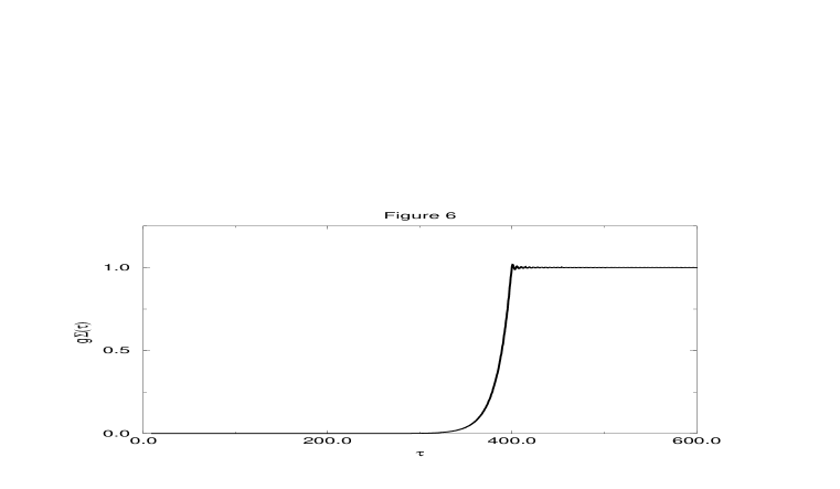
FIG. 6.: $g\Sigma$ vs. $\tau$, for $\eta(0)=0,\dot{\eta}(0)=0,g=10^{-14},h_{0}=10.0$.

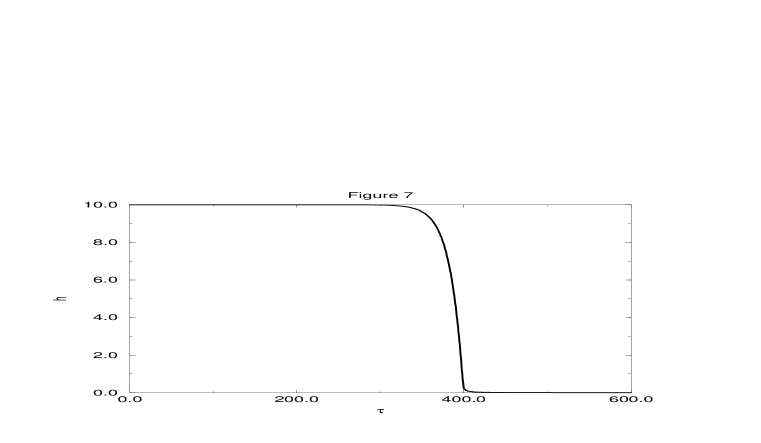
FIG. 7.: $H(\tau)$ vs. $\tau$, for $\eta(0)=0,\dot{\eta}(0)=0,g=10^{-14},h_{0}=10.0$.

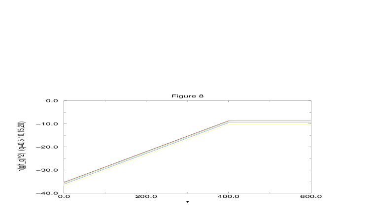
FIG. 8.: $\ln(|f_{q}(\tau)|^{2})$ vs. $\tau$, for $\eta(0)=0,\dot{\eta}(0)=0,g=10^{-14},h_{0}=10.0$ for $q=0.0,5,10,15,20$ with smaller $q$ corresponding to larger values of $\ln(|f_{q}(\tau)|^{2})$.

FIG. 9.: $p/\varepsilon$ vs. $\tau$, for $\eta(0)=0,\dot{\eta}(0)=0,g=10^{-14},h_{0}=10.0$.

FIG. 10.: ${\cal F}(H/m)$ vs. $H$, where ${\cal F}(H/m)$ is defined by the relation $\phi_{eff}(0)=(H/2\pi){\cal F}(H/m)$ (see eqs. (97) and (98)).

FIG. 11.: $\eta_{eff}^{2}(\tau)$ vs. $\tau$, for $\eta_{eff}(0)=3.94\times 10^{-7},\dot{\eta}_{eff}(0)=0.317\eta_{eff}(0),g=10^{-14},h_{0}=2.0$. The initial conditions were obtained by fitting the intermediate time regime of $g\Sigma(\tau)$ in fig. (1). $\eta_{eff}(\tau)$ is the solution of eq.(99) with these initial conditions.

FIG. 12.: $h(\tau)$ vs. $\tau$, obtained from the solution of eqns. (99) and (102) with the conditions of fig. (11)).

REFERENCES

- [1] A. H. Guth, Phys. Rev. D23, 347 (1981).
- [2] “The Scalar, Vector and Tensor Contributions to CMB anisotropies from Topological Defects”, by N. Turok, Ue-Li Pen, U. Seljak astro-ph/9706250 (1997).
- [3] “The case against scaling defect models of cosmic structure formation” by Andreas Albrecht, Richard A. Battye, James Robinson, astro-ph/9707129 (1997).
- [4] “CMB Anisotropy Induced by Cosmic Strings on Angular Scales ”, by B. Allen, R. R. Caldwell, S. Dodelson, L. Knox, E. P. S. Shellard, A. Stebbins, astro-ph/9704160 (1997).
- [5] For thorough reviews of standard and inflationary cosmology see: E. W. Kolb and M. S. Turner, The Early Universe (Addison Wesley, Redwood City, C.A. 1990). A. Linde, Particle Physics and Inflationary Cosmology, (Harwood Academic Pub. Switzerland, 1990). R. Brandenberger, Rev. of Mod. Phys. 57,1 (1985); Int. J. Mod. Phys. A2, 77 (1987).
- [6] For more recent reviews see: M. S. Turner, astro-ph/9703197; astro-ph/9703196; astro-ph/9703174; astro-ph/9703161; astro-ph/9704062; astro-ph/9704024. A. Linde, in Current Topics in Astrofundamental Physics, Proceedings of the Chalonge Erice School, N. Sánchez and A. Zichichi Editors, Nato ASI series C, vol. 467, 1995, Kluwer Acad. Publ.
- [7] A. R. Liddle, astro-ph/9612093, Lectures at the Casablanc Winter School Morocco, 1996.
- [8] A. R. Liddle and D. H. Lyth, Phys. Rep. 231, 1 (1993).
- [9] G. Smoot, astro-ph/9705135; M. Sakellariadou, astro-ph/9612075, and references therein.
- [10] D. H. Lyth, hep-ph/9609431 (1996).
- [11] S. Dodelson, W. H. Kinney and E. W. Kolb, Phys. Rev. D56, Sept. 15, 1997 (astro-ph/9702166).
- [12] D. Boyanovsky, H. J. de Vega, R. Holman, D.-S. Lee and A. Singh, Phys. Rev. D51, 4419 (1995); D. Boyanovsky, H. J. de Vega, R. Holman and J. F. J. Salgado, Phys. Rev. D54, 7570, (1996); D. Boyanovsky, H. J. de Vega and R. Holman in the Proceedings of the Erice Chalonge School on Astrofundamental Physics, p. 183-270, N. Sánchez and A. Zichichi eds., World Scientific, 1997.
- [13] D. Boyanovsky, H. J. de Vega and R. Holman, Phys. Rev. D49, 2769 (1994).
- [14] D. Boyanovsky, D. Cormier, H. J. de Vega and R. Holman, Phys. Rev D55, 3373 (1997).
- [15] D. Boyanovsky, D-S. Lee, and A. Singh, Phys. Rev. D48, 800 (1993).
- [16] D. Boyanovsky, D. Cormier, H. J. de Vega, R. Holman, A. Singh, M. Srednicki, Phys. Rev. D56, 1939 (1997).
- [17] A.D. Linde, Phys. Lett. B116, 335 (1982).
- [18] A. Vilenkin, Phys. Lett. B115, 91 (1982).
- [19] P. J. Steinhardt and M. S. Turner, Phys. Rev. D29, 2162, (1984).
- [20] A. Guth and S-Y. Pi, Phys. Rev. D32, 1899 (1985).
- [21] N. D. Birrell and P.C.W. Davies, ‘Quantum fields in curved space’ Cambridge Univ. Press, (Cambridge, 1986).
- [22] O. Eboli, R. Jackiw and S-Y. Pi, Phys. Rev. D37, 3557 (1988); M.Samiullah, O. Eboli and S-Y. Pi, Phys. Rev. D44, 2335 (1991).
- [23] J. Guven, B. Liebermann and C. Hill, Phys. Rev. D39, 438 (1989).
- [24] For non-equilibrium methods in different contexts see for example: F. Cooper, J. M . Eisenberg, Y. Kluger, E. Mottola, B. Svetitsky, Phys. Rev. Lett. 67, 2427 (1991); F. Cooper, J. M. Eisenberg, Y, Kluger, E. Mottola, B. Svetitsky, Phys. Rev. D48, 190 (1993).
- [25] F. Cooper and E. Mottola, Mod. Phys. Lett. A 2, 635 (1987); F. Cooper, S. Habib, Y. Kluger, E. Mottola, J. P. Paz, P. R. Anderson, Phys. Rev. D50, 2848 (1994). F. Cooper, S.-Y. Pi and P. N. Stancioff, Phys. Rev. D34, 3831 (1986). F. Cooper, Y. Kluger, E. Mottola, J. P. Paz, Phys. Rev. D51, 2377 (1995). F. Cooper and E. Mottola, Phys. Rev. D36, 3114 (1987).
- [26] S. A. Ramsey, B. L. Hu, Phys. Rev. D56, 678 (1997).
- [27] J. Baacke, K. Heitmann and C. Patzold, hep-ph/9706274; Phys.Rev. D55 (1997) 2320.
- [28] D. Polarski and A. A. Starobinsky, Class. Quant. Grav. 13, 377 (1996); J. Lesgourgues, D. Polarski and A. A. Starobinsky, Nucl. Phys. B497, 479 (1997) and references therein.
- [29] L. P. Grishchuk, Phys. Rev. D 45, 4717 (1992).
- [30] V. F. Mukhanov, H. A. Feldman and R. H. Brandenberger, Phys. Rep. 215, 293 (1992).
- [31] J. Bardeen, Phys. Rev. D22, 1882 (1980).
- [32] R. R. Caldwell, Class. Quant. Grav. 13, 2437 (1995).
- [33] J. Martin and D. J. Schwarz, gr-qc-9704049 (1997).
- [34] K. M. Gorski, A. J. Banday, C. L. Bennett, G. Hinshaw, A. Kogut and G. F. Smoot, (astro-ph/9601063) (submitted to ApJ. Lett.).
- [35] L. P. Grishchuk, Phys. Rev. D. 52, 5549, (1995); Proceedings of the NATO Advanced Study Institute on “String Gravity and Physics at the Planck Scale”, Ed. N. Sanchez and A. Zichichi. (NATO ASI series, Kluwer, 1996), page 369; Phys. Rev. D53 (1996) 6784; Proceedings of the NATO Advanced Study Institute on “Current Topics in Astrofundamental Physics: the Early Universe”, Ed. N. Sanchez and A. Zichichi. (NATO ASI series, Kluwer, 1995), page 205 ( gr-qc/9511074).
- [36] J. E. Lidsey, A. R. Liddle, E. W. Kolb, E. J. Copeland, T. Barreiro, M. Abney, Rev. Mod. Phys. 69, 373, (1997).
- [37] E. D. Stewart and D. H. Lyth, Phys. Lett. B302, 171 (1993).
- [38] S. Habib, Phys. Rev. D 46, 2408 (1992); Phys. Rev. D 42, 2566, (1990); S. Habib and R. Laflamme, Phys. Rev. D42, 4056, (1990), and references therein.
- [39] See eq.(53) in the first reference under [28].