TAUP  2450 - 97

DESY   97 - 171

September 1997

WHERE ARE THE BFKL POMERON
and
SHADOWING CORRECTIONS IN DIS ?

Eugene Levin

School of Physics and Astronomy, Tel Aviv University

Ramat Aviv, 69978, ISRAEL

and

DESY Theory, Notkestr. 85, D - 22603, Hamburg, GERMANY

leving@ccsg.tau.ac.il;   levin@mail.desy.de;

Talk given at the RIKEN BNL WS on “ Perturbative QCD as a Probe of Hadron Structure”, BNL LI July 14 - 25,1997.

Abstract: In this talk, I will argue that the HERA experimental data show that the typical parameter ($\kappa$) responsible for the value of the shadowing corrections (SC) in DIS is so large that the BFKL Pomeron is hidden under SC. The SC turn out to be large enough but mostly for the gluon structure function which is not well determined by the available experimental data and by the current theoretical procedure.

In this talk I am going to answer two questions:

Q1: Where is the BFKL [2] Pomeron?

Q2: Where are shadowing corrections (SC)?

Actually, the answers have been presented in our paper [1], but here I will discuss them in more details.

First, let me explain why it is reasonable to ask such questions. Indeed, at first sight, the situation looks very transparent, namely, the HERA data can be described by means of the usual DGLAP [3] evolution equations without any other ingredients such as the BFKL Pomeron and / or SC ( see any of plenary talks during the past three years). My personal opinion is that this fact brought more questions than answers since we need to show ( to justify theoretically our approach) that the corrections due to the BFKL dynamics and/or due to the SC are negligible small at least at the HERA kinematic region. If it is not so ( as I will show below) the DGLAP approach is not better or worse than any other model developed to describe the experimental data. The main goal of this talk is to show that the experimental data from HERA confirm that both the BFKL contribution and the SC should be rather large in the HERA kinematic region.

Actually, everything that I want to tell is given in Fig.1, but I need to explain what are plotted in this figure.

1. $<\gamma>\,=\,\frac{1}{2}$ and $<\gamma>\,=\,1$.

Let me recall a standard procedure of solving of the DGLAP evolution equations.

The first step: we introduce moments of the structure function, namely,

$$xG(x,Q^{2})\,=\,\frac{1}{2\pi i}\int_{C}e^{-\omega\,\ln(1/x)}\,M(\omega,Q^{2})\,d\omega,$$

where contour $C$ is located to the right of all singularities of moment $M(\omega,Q^{2})$.

The second step: we find the solution to the DGLAP equation for moment

$$\frac{dM(\omega,Q^{2})}{d\ln Q^{2}}\,\,=\,\,\gamma(\omega)\,M(\omega,Q^{2})\,\,.$$ (1)

The solution is

$$M(\omega,Q^{2})\,\,=\,\,M(\omega,Q^{2}_{0})\,\cdot\,e^{\gamma(\omega)\,\ln(Q^{2}/Q^{2}_{0})}\,\,.$$ (2)

Here $M(\omega,Q^{2}_{0})$ is the nonperturbative input which should be taken from experimental data or from “soft” phenomenology ( model).

The third step: we find the solution for the parton structure function using the inverse transform, namely:

$$xG(x,Q^{2})\,\,=\,\,\int_{C}\,\frac{d\omega}{2\pi i}\,\,e^{\omega\,\ln(1/x)\,+\,\gamma(\omega)\,\ln(Q^{2}/Q^{2}_{0})}\,M(\omega,Q^{2}_{0})\,\,.$$ (3)

Therefore, to find a solution of the DGLAP equation we need to know the nonperturbative input $M(\omega,Q^{2}_{0})$ and the anomalous dimension $\gamma(\omega)$, which we can calculate in perturbative QCD. The anomalous dimension $\gamma(\omega)$ has been calculated in pQCD and the result of calculations can be written in the form:

$$\gamma(\omega)\,\,=\,\,\gamma^{BFKL}(\frac{\alpha_{S}N_{c}}{\pi\,\omega})\,\,-\,\,\frac{\alpha_{S}N_{c}}{\pi\,\omega}\,\,+\,\,\alpha_{S}\,\gamma_{1}(\omega)\,\,+\,\,\alpha^{2}_{S}\,\gamma_{2}(\omega)\,\,,$$ (4)

where both functions $\gamma_{1}$ and $\gamma_{2}$ are known as well as $\gamma^{BFKL}$. Using Eq. (4) we can discuss what has been done in the global fits [4]. The value of the anomalous dimension has been calculated in $\alpha_{\rm S}$ and $\alpha^{2}_{S}$ orders ( two last terms in Eq.(5)) and the nonperturbative input has been taken in the form $M(\omega,Q^{2}_{0})\,\propto\,\frac{1}{\omega-\omega_{0}}$ with $\omega_{0}\,\approx\,$ 0.2 - 0.3. This means that the structure function at $Q^{2}=Q^{2}_{0}$ increases as $x^{-\omega_{0}}$ at $x\rightarrow 0$ . However, one can see that the $\gamma^{BFKL}$ should be essential in the region of low $x$ where $\omega\,\rightarrow\,0$ since

$$\gamma^{BFKL}(\frac{\alpha_{s}N_{c}}{\pi\,\omega})\,\,=\,\,\frac{\alpha_{s}N_{c}}{\pi\,\omega}\,\,+\,\,\sum_{n=4}\,C_{n}\,(\,\frac{\alpha_{s}N_{c}}{\pi\,\omega}\,)^{n}\,\,\rightarrow\,|_{\omega\,\rightarrow\,0}\,\,\frac{1}{2}\,\,+\,\,\sqrt{\frac{\omega\,-\,\omega_{L}}{\Delta}}\,\,,$$ (5)

where $\omega_{L}$ and $\Delta$ have been calculated [2].

This equation reflects the main properties of the BFKL Pomeron: the limited value of the anomalous dimension and the importance of all terms of the order of $(\frac{\alpha_{s}N_{c}}{\pi\,\omega})^{n}$ in the region of small $\omega$. All attempts to estimate the values of the BFKL terms in the anomalous dimension [5] show that they are essential in the HERA kinematic region. Here, we choose a different way of presentation of this well known fact, namely, we introduce average anomalous dimension $<\gamma>$ which is equal to

$$<\gamma>\,\,=\,\,\frac{1}{xG(Q^{2},x)}\cdot\frac{\partial xG(Q^{2},x)}{\partial\ln(Q^{2}/Q^{2}_{0})}\,\,=\,\,\frac{\int_{C}\,\frac{\gamma(\omega)\,\,d\omega}{2\pi i}\,\,e^{\omega\,\ln(1/x)\,+\,\gamma(\omega)\,\ln(Q^{2}/Q^{2}_{0})}\,M(\omega,Q^{2}_{0})}{\,\int_{C}\,\frac{d\omega}{2\pi i}\,\,e^{\omega\,\ln(1/x)\,+\,\gamma(\omega)\,\ln(Q^{2}/Q^{2}_{0})}\,M(\omega,Q^{2}_{0})}\,\,.$$ (6)

Function $<\gamma>$ describes the behaviour of the anomalous dimension quite well since at low $x$ the deep inelastic structure functions can be calculated in the semiclassical approach [6] in which, for example $xG(Q^{2},x)$, is equal to

$$xG(Q^{2},x)\,\,=\,\,C(\ln(1/x),\ln(Q^{2}/Q^{2}_{0}))\,\cdot\,\frac{1}{x^{<\omega(\ln(1/x),\ln(Q^{2}/Q^{2}_{0}))>}}\,\cdot\,(\frac{Q^{2}}{Q^{2}_{0}})^{<\gamma(\ln(1/x),\ln(Q^{2}/Q^{2}_{0}))>}\,\,$$ (7)

where functions $C$,$<\omega>$ and $<\gamma>$ are smooth function of $\ln(1/x)$ and $\ln(Q^{2}/Q^{2}_{0})$.

In Fig.1 we plotted two lines with $<\gamma>$  =  $\frac{1}{2}$ and $<\gamma>$ = 1 . We expect a large the BFKL contribution in the kinematic region between these two lines and one can see in Fig.1 that we have penetrated this region at HERA.

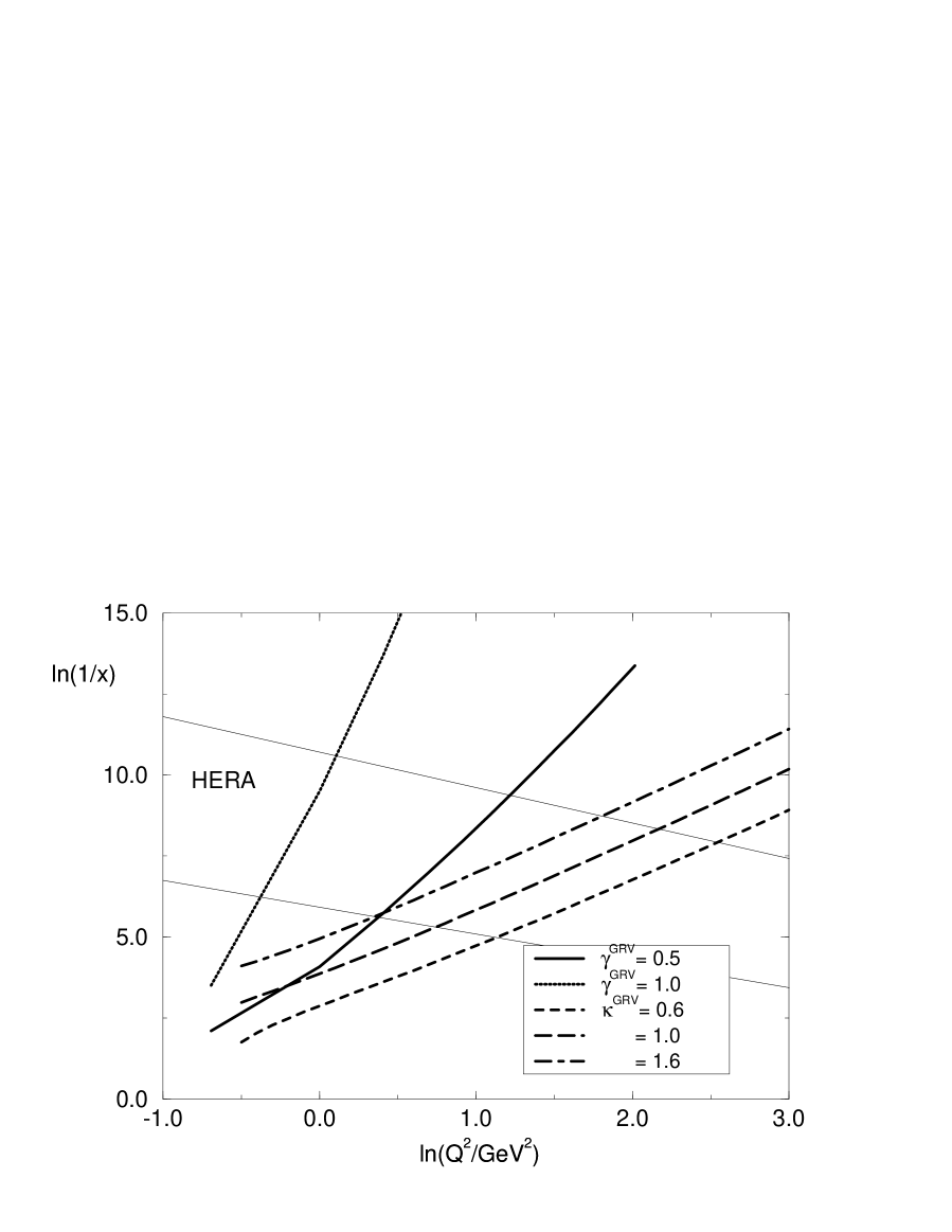
Figure 1: Contours for $<\gamma>$ = 1 and 1/2 and $\kappa$ = 0.6,1,1.6 for the GRV95 gluon density and HERA kinematic region.

2. $\kappa$.

From HERA data we can evaluate also the probability $\kappa$ of the parton - parton (gluon - gluon) interaction, which is given by [6], [7]

$$\kappa\,\,=\,\,xG(x,Q^{2})\frac{\sigma(GG)}{Q^{2}\,\pi R^{2}}\,\,=\,\,\frac{3\,\pi\,\alpha_{S}}{Q^{2}\,R^{2}}\,\,xG(x,Q^{2})\,\,,$$ (8)

where $xG(x,Q^{2})$ is the number of partons ( gluons) in the parton cascade and $R^{2}$ is the radius of the area populated by gluons in a nucleon. $\sigma(GG)$ is the gluon cross section inside the parton cascade and was evaluated in [7].

The observation is that we know from the HERA data both the value of the gluon structure function and the value of $R^{2}$ in Eq. (8). Indeed, the available parameterizations such as MRS, CTEQ and GRV [4] give the value of the gluon structure function with sufficiently large differences in its value. However, this difference is less than 50% and becomes smaller with improvement of the experimental data on $F_{2}(x,Q^{2})$ ( see Fig.2 ).

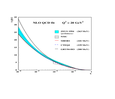
Figure 2: The value of the gluon structure function in different parameterizations.

The most important and new information is the fact that using HERA data on photoproduction of J/$\Psi$ meson [8] the value of $R^{2}$ can be estimated as $R^{2}\,\,\leq\,\,5\,GeV^{-2}$ [9].

Figure 3: The J/$\psi$ production without (a) and with ( b) proton dissociation.

Indeed, (i) the experimental values for the slopes ( see Fig.3 ) are $B_{el}\,=\,4\,GeV^{-2}$ and $B_{in}\,=\,1.66\,GeV^{-2}$ and (ii) the cross section for J/$\Psi$ production with and without proton dissociation are equal [8]. Taking into account both facts we can estimate the value of $R^{2}$ ( see Ref.[9] for details) which appears in calculation of the SC (Glauber corrections) due to integration over the momentum transferred ($q^{2}_{\perp}\,=\,|t|$) along the gluon ladders (see Fig.4) neglecting $t$ dependence of the upper vertex in Fig.4.

In Fig.3 we show the picture for the diffractive production of J/$\Psi$ in the additive quark model, in which two radii naturally appear as the radius of the hadron and a proper radius of the constituent quark. In all our estimates we did not need this particular model but it is interesting to mention that our estimates give the same value of the average radius as in the additive quark model.

It should be stressed that such an estimate gives the value for $R^{2}$ which lead to the value of the cross section for the double parton scattering measured by the CDF collaboration at the Tevatron [10].

Figure 4: The SC for the total cross section of $\gamma^{*}p$ interaction.

Let us discuss this point a little bit in more details. The CDF collaboration measured the processes of unclusive production of two pairs of “hard” jets with almost compensated transverse momenta in each pair and with almost the same values of rapidities. Such pairs can be produced only due to double parton collision and their cross section can be calculated using the Mueller diagram given in Fig.5.

Figure 5: Inclusive production of two pair of “hard” jets in the double parton scattering.

The value of the double parton scattering cross section can be written in the form ( see Fig.5)[10]:

$$\sigma_{DP}\,\,=\,\,m\,\,\frac{\sigma(\bar{Q}_{1}Q_{1})\,\,\sigma(\bar{Q}_{2}Q_{2})}{2\,\sigma_{eff}}\,\,,$$ (9)

where, for simplicity, we consider the production of two ( $\bar{Q}_{1}Q_{1}$ and $\bar{Q}_{2}Q_{2}$ ) quark - antiquark pairs. Factor $m$ in Eq. (9) is equal to 2 for different quarks ( $Q_{1}\,\neq\,Q_{2}$) and to 1 for identical quarks. The value for $\sigma_{eff}$ is measured to be 14.5 $\pm$ 1.7 $\pm$ 2.3 mb. Our estimates [11] for diagrams of Fig.5 using the two radii picture give $\sigma_{eff}\,\sim\,17mb$. It means that the effective radius $R^{2}=5GeV^{-2}$ could be even overestimated.

Using the GRV parameterization for the gluon structure function and the value of $R^{2}=5\,GeV^{-2}$, we obtain that $\kappa$ reaches 1 at HERA kinematic region ( see Fig.1 ), meaning shadowing corrections should not be neglected. In Fig.1 we plotted three curves with values of $\kappa$ equal to 1.6, 1 and 0.6, respectively, to illustrate a possible range of $\kappa$ using CTEQ and MRS parameterizations.

A1:

The answer to the first question one can read from Fig.1. Indeed, the kinematic region where the BFKL Pomeron ( the BFKL corrections to the anomalous dimension ) could be sizeable, namely, the region between curves $<\gamma>$ = 1/2 and $\gamma$ = 1 , is located to the left of the curve with $\kappa$ = 1 where the SC should be essential. Therefore, we can conclude that the BFKL Pomeron is hidden under large SC and cannot be observed. To illustrate this point and to show what is the influence of the SC on the behaviour of the average anomalous dimension we plotted in Fig.6 $<\gamma>$ given by Eq.(6) but using the Glauber - Mueller formula for the SC for the gluon structure function ( see Ref. [1] ). The calculations were performed for the gluon structure function at fixed impact parameter ($b_{t}=0$), where we take

$$xg(x,Q^{2})\,=\,\int d^{2}b_{t}S(b_{t})xG(x,Q^{2})\,\,,$$

with

$$S(b_{t})\,\,=\,\,\frac{1}{\pi R^{2}}e^{-\,\frac{b^{2}_{t}}{R^{2}}}\,\,.$$

One can see, that the average anomalous dimension turns out to be smaller that $<\gamma>\,=\,\frac{1}{2}$. Therefore, the BFKL Pomeron will not be seen even if we will take the SC at the minimal rate given the Glauber - Mueller formula.

A2:

It turns out that the SC is not very big for $F_{2}(Q^{2},x)$ which has been measured experimentally ( see Ref.[1] for details). However, the SC for $xG(Q^{2},x)$ should be large. To illustrate this point we plot in Fig.6 the ratio $R_{1}\,=\,\frac{xG(Q^{2},x)^{SC}}{xG(Q^{2},x)^{GRV}}$ calculated in Ref. [1]. Comparing Fig.6 with the value of $xG(Q^{2},x)$ in current parameterizations we can conclude that in spite of sufficiently large SC our knowledge of the value of the gluon structure function is so poor that we can absorb all SC in the uncertainties of its value. For example, taking into account the SC the GRV gluon structure function will be able to describe the new experimental data while without the SC the GRV parameterization has been ruled out by experiment ( see the last picture in Fig.2.).

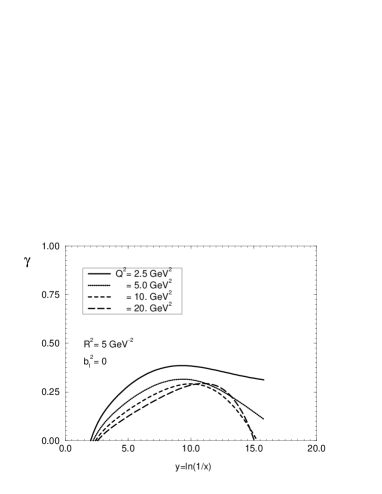
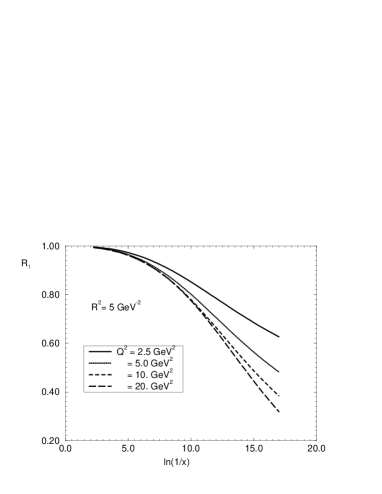
Figure 6: Average anomalous dimension, given in Eq.(6) for the SC taken in Mueller-Glauber formula for $b_{t}=0$ and ratio $R_{1}$ for the gluon structure function.

It should be stressed, that our answers bring several problems that have to be solved in the nearest future. These are three of them:

P1:

It is very likely that the BFKL Pomeron will be hidden under SC not only for the deep inelastic proton structure function but in all specially invented processes to extract the BFKL Pomeron since the typical size ( the value of $R^{2}$) is smaller in all such processes than in the case of the deep inelastic structure function.

P2:

The fact that the SC will take place of the BFKL Pomeron does not mean that the the experimental cross section will be the same as in the DGLAP evolution equations or in the Monte Carlo simulations based on the DGLAP evolution. The difference should be calculated to be discussed.

P3:

The size of the SC for the gluon structure function crucially depends on the initial gluon distribution. In our estimates we pretended that the GRV parameterization guessed correctly this initial distribution. The only argument is the fact that the GRV parameterization describes the experimental $F_{2}(x,Q^{2})$ at small $Q^{2}\,\approx\,1\,GeV^{2}$.

Alternative answers:

AA1:

The first alternative answer has been proposed by R. Thorne (see Ref. [12] ) who demonstrated that the correct inclusion of the BFKL anomalous dimension allows to improve the comparison with the experimental data. However, Fig.7 shows that the value of the gluon structure function extracted from the experimental data is not very different from the previous analysis without the BFKL anomalous dimension. Therefore, the experimental data, perhaps, does not contradict the existence of the BFKL Pomeron, but this fact cannot change considerably the value of $\kappa$. It means, that the value of the SC is still big even in the analysis taking into account the BFKL Pomeron ( see KMS paper [12] for details). In Fig.7 is given some next to leading order corrections to the BFKL Pomeron. One can see that they are essential and diminish the value of the gluon structure function but still not more than in two times, which we evaluate as a typical error in the value of extracted gluon structure function.

Figure 7: The gluon structure function with and without the BFKL Pomeron ( picture is taken from the KMS paper [12]).

AA2:

The BFKL Pomeron is not seen in the data because the next to leading correction is essential and they change crucially the main properties of the BFKL Pomeron. Fortunately, the next order correction to the BFKL Pomeron (NOBFKL) has been calculated [13] and the community of experts has started to understand the influence of the NOBFKL [14] [15] on the value of the gluon structure function. It turns out the the NOBFKL Pomeron has a much smaller intercept or in other word the power - like behaviour, namely, $xG*x,Q^{2})\,\,\propto\,\,(\frac{1}{x_{B}})^{\omega_{L}}$, still remains but $\omega_{l}^{NO}\,\,=\,\,\omega^{LO}_{L}(\,1\,\,-\,\,3.4\,\alpha_{\rm S}\,)$. It means that the energy ( $x$) dependence becomes milder and it makes the NOBFKL Pomeron not so pronounced as it was in the leading order. Nevertheless, the first numerical estimates show that the value of the gluon structure function changes but not significally. Indeed, Fig.8 that was taken from Ref.[15] shows that the gluon structure function in the analysis with the NOBFKL anomalous dimension typically on 30% less than the gluon structure function without the BFKL contribution.

Figure 8: The gluon structure function with and without the NOBFKL Pomeron ( picture is taken from the Blumlein and Vogt paper [15]).

My conclusions:

These two examples of the alternative answer show that (i) it is not so easy to change significally the value of the gluon structure function and diminish it more than in two times; and (ii) the real accuracy of the value of the gluon structure function is rather big, about 50%, in spite of the fact that the difference between two sets of gluon structure functions ( so called global fits: MRS and CTEQ ) became much smaller using new more accurate experimental data (see Fig.2). Our errors are mostly theoretical ones. In my opinion, we cannot change ( diminish ) the value of parameter $\kappa$ and therefore, accordingly to Fig.1, we have to deal first with the SC and only after that to take into account the BFKL Pomeron with all possible corrections.

Finally, I would like to emphasize that you got my personal answers. Perhaps, you have different ones. The only point, which I insist on, is that, before answering these two questions, we cannot trust the DGLAP evolution more than any other model.

References

- [1] A.L.Ayala,M.B. Gay Ducati and E.M.Levin: TAUP-2432-97,hep-ph/9706347.
- [2] E.A. Kuraev, L.N. Lipatov and V.S. Fadin: Sov. Phys. JETP 45(1977) 199 ; Ya.Ya. Balitskii and L.V. Lipatov: Sov.J. Nucl. Phys. 28 (1978) 822; L.N. Lipatov: Sov. Phys. JETP 63 (1986) 904.
- [3] V.N. Gribov and L.N. Lipatov:Sov. J. Nucl. Phys. 15 (1972) 438; L.N. Lipatov: Yad. Fiz. 20 (1974) 181; G. Altarelli and G. Parisi:Nucl. Phys. B126 (1977) 298; Yu.L. Dokshitser:Sov. Phys. JETP 46 (1977) 641.
- [4] M. Gluck, E. Reya and A. Vogt: Z.Phys. C67(1995)433; A.D. Martin, R.G. Roberts and W.J. Stirling: Phys.Lett.B306(1993)145; CTEQ Collaboration, H.L.Lai et al.: Phys.Rev.D51(1995) 4763.
- [5] R.K. Ellis, Z. Kunst and E. M. Levin: Nucl. Phys.B420(1994) 517;R.S.Thorne: hep - ph /9701241 and references therein; J. Kwiecinski, A.D. Martin and A.M. Stasto: hep - ph /9703445.
- [6] L.V. Gribov, E.M. Levin and M.G. Ryskin: Phys. Rep. 100 (1983) 1.
- [7] A.H. Mueller and J. Qiu: Nucl. Phys. B268 (1986) 427.
- [8] H1 Collaboration; S.Aid et al.: Nucl. Phys.B472(1996)3; ZEUS Collaboration; M.Derrick et al.: Phys. Lett.B350(1995)120.
- [9] A.L.Ayala,M.B. Gay Ducati and E.M.Levin: Phys. Lett. B388 (1996)188; E. Gotsman,E.Levin and U. Maor: Phys. Lett. 403 (1997) 120.
- [10] CDF Collaboration, F.Abe et al.: FERMILAB-Pub-97/083-E.
- [11] E. Gotsman,E.Levin and U. Maor: in preparation.
-
[12]
R. Thorne, Phys. Lett. B392 (1997) 463; hep-ph/9701241; hep -
ph/9706233; hep - ph/9708302;
J. Kwiecinsci,A.D. Martin and A. M. Stasto: hep - ph/9703445;
I. Bojak and M. Ernst, Phys. Lett. B397 (1997) 296; hep-ph/9702282. -
[13]
V.S. Fadin and L.N. Lipatov: Yad. Fiz. 50 (1989) 1141; Nucl. Phys. B406 (1993) 259, B477 (1996) 767;
V.S. Fadin, R.Fiore and A. Quartarolo: Phys. Rev. D50 (1994) 2265,5893;
V.S.Fadin, R. Fiore and M.I. Kotsky: Phys. Lett. B359 (1995) 181, B387 (1996) 593, B389 (1996) 737;
V.S. Fadin, L.N. Lipatov and M.I. Kotsky: hep - ph /9704267;
V.S. Fadin: talk at DIS’97, Chicago, April 1997. - [14] G. Camici and M. Ciafaloni, Phys. Lett. B386 (1996) 34; hep-ph/9707390.
- [15] J. Blumlein and A. Vogt: DESY 97 - 143; hep - ph/9707488.