On the Analytic “Causal” Model for the QCD Running Coupling

Abstract

We discuss the model $\bar{\alpha}_{\rm an}(Q^{2})$ recently proposed for the QCD running coupling $\bar{\alpha}_{s}(Q^{2})$ in the Euclidean domain on the basis of the “asymptotic–freedom” expression and on causality condition in the form of the $Q^{2}$-analyticity.

The model contains no adjustable parameters and obeys the important features: (i) Finite ghost-free behavior in the “low $Q^{2}$” region and correspondence with the standard RG-summed UV expressions;(ii) The universal limiting value $\bar{\alpha}_{\rm an}(0)$ expressed only via group symmetry factors. This value as well as the $\bar{\alpha}_{\rm an}$ behavior in the whole IR region $Q^{2}\leq\Lambda^{2}$ turns out to be stable with respect to higher loop corrections; (iii) Coherence between observed $\bar{\alpha}_{s}(M_{\tau}^{2})$ value and integral information on the IR $\bar{\alpha}_{s}(Q^{2})$ behavior extracted from jet physics.

1 INTRODUCTION

This presentation is devoted to the review and discussion of a new analytized model expression $\bar{\alpha}_{\rm an}(Q^{2})$ for the QCD running coupling recently devised [1] by combining the RG-summed expression $\bar{\alpha}_{s}(Q^{2})$ with the demand of analyticity, that is causality, in the $Q^{2}$ complex plane. This procedure ”cures” the IR ghost-pole trouble by an additional contribution that is non-analytic in the coupling constant and at the same time preserves the asymptotic freedom property and correspondence with perturbation theory in the UV .

The “analytization procedure” elaborated in the mid-fifties (see Ref.[2]) consists of three steps:

– Find an explicit expression for $\bar{\alpha}_{RG}(Q^{2})$ in the Euclidean region $Q^{2}>0$ by standard RG improvement of a perturbative input.

– Perform the straightforward analytical continuation of this expression into the Minkowskian region ${\rm Re}\,Q^{2}<0,{\rm Im}\,Q^{2}=-\epsilon$. Calculate its imaginary part and define the spectral density by $\rho_{RG}(\sigma,\alpha)={\rm Im}\bar{\alpha}_{RG}(-\sigma-i\epsilon,\alpha)$.

– Using the spectral representation of the Källen–Lehmann type with $\rho_{RG}$ in the integrand, define an “analytically-improved” running coupling $\bar{\alpha}_{\rm an}(Q^{2})$ in the Euclidean region.

Being applied to $\bar{\alpha}(Q^{2})$ in the one- and two-loop QED {or QCD} case, this procedure produces (see Ref. [2] {or  [1, 3]}) an expression $\bar{\alpha}_{\rm an}(Q^{2})$ with the properties:

(a) it has no ghost pole,

(b) in the complex $\alpha$-plane at the point $\alpha=0$ it possesses an essential singularity $\sim\exp(-1/\alpha\beta_{1})$, with $\beta_{1}$, the one-loop beta-function coefficient,

(c) in the vicinity of this singularity for real and positive $\alpha$ it admits a power expansion that coincides with the perturbation input,

(d) it has the finite UV {or IR} limit $4\pi/\beta_{1}$ that does not depend on the experimental value $\alpha\simeq 1/137$ {or $\Lambda\}$.

In the one-loop QCD case this expression is of the form

$$\bar{a}^{(1)}_{\rm an}(Q^{2})=\frac{1}{\ln Q^{2}/\Lambda^{2}}\,+\,\frac{\Lambda^{2}}{\Lambda^{2}-Q^{2}}$$ (1)

with $\bar{a}=\beta_{1}\bar{\alpha}_{s}/4\pi$ and $\beta_{1}=11-(2/3)n_{f}$.

The same procedure being applied to the two-loop case yields [2, 1, 3] a more complicated expression with the same essential features (see, e.g., Eqs. (6) - (9) below).

2 THE MODEL FOR QCD RUNNING COUPLING

The  “analytic” coupling constant, Eq. (1), instead of ghost pole has a weak singularity at $Q^{2}=0$ and its IR limit $\bar{\alpha}_{s}^{(1)}(0)=4\pi/\beta_{1}$ depends only on group factors. Numerically, for $n_{f}=3$,we have $\bar{\alpha}_{\rm an}^{(1)}(0)=4\pi/9\simeq 1.4$.

Note, to relate $\Lambda$, the QCD scale parameter, to $a(\mu^{2})$, in our case we have to change its usual one-loop definition for $\Lambda^{2}=\mu^{2}\exp[-\phi(a(\mu^{2}))]$ with the function $\phi$ defined by the transcedental relation

$$a=1/{\phi(a)}-1/[\exp(\phi(a))-1]~{}\,$$ (2)

which is consistent with the symmetry property

$$\ \phi(a)=-\phi(1-a)\,.$$ (3)

The corresponding beta-function

$$\beta(a)=-\frac{1}{\phi^{2}(a)}+\frac{\exp{\phi(a)}}{\left[\exp{\phi(a)}-1\right]^{2}}$$ (4)

is also symmetric $\beta(a)=\beta(1-a)$ and obeys the second-order zero at $a=1$ – see Fig. 1.

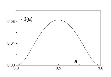
Figure 1: One-loop $\beta(a)$ function.

Usually, in perturbative QFT practice, we are accustomed to the idea that theory supplies us with a set of possible curves for $\bar{\alpha}_{s}(Q)$ and one has to fix the “physical one” by comparing with experiment. Here, Eq. (1) describes a family of such curves for $\bar{\alpha}_{\rm an}(Q^{2})$ forming a bundle with the same common limit at $Q^{2}=0$.

For the two-loop case, we start with the running coupling written down in the form

$$\bar{a}^{(2)}_{RG}(Q^{2})=\frac{1}{l+b\ln(1+l/b)}~{},\quad l=\ln\frac{Q^{2}}{\Lambda^{2}}\,,$$ (5)

with $b=\beta_{2}/(\beta_{1})^{2}$ and $\beta_{2}=102-38/3n_{f}$. This expression corresponds to the result of exact integration of the two-loop differential RG equation explicitly resolved by iteration. It generates a popular two-loop formula with the $\ln l/l^{2}$ term. For the spectral density, we have

$$\rho^{(2)}_{RG}(L)\,=\,\frac{I(L)}{R^{2}(L)\,+\,I^{2}(L)}\,,\quad L=\ln\frac{\sigma}{\Lambda^{2}}$$ (6)

with

$$R(L)=L+b\ln\sqrt{(1+L/b)^{2}+(\pi/b)^{2}}~{},$$ (7)

$$I(L)=\pi+b\arccos\frac{b+L}{\sqrt{\left(b+L\right)^{2}+\pi^{2}}}~{}.$$ (8)

Now, to obtain $\bar{a}^{(2)}_{\rm an}(Q^{2})$, one has to substitute Eq. (6) into the r.h.s. of

$$\bar{a}_{\rm an}(Q^{2})=\frac{1}{\pi}\int_{0}^{\infty}d\sigma\frac{\rho(\sigma,a)}{\sigma+Q^{2}-i\epsilon}\,.$$ (9)

The one-loop result, Eq.(1), follows from Eqs. (6) - (9) at $b=0$. However, in the two-loop case, the integral expression thus obtained is too complicated for being presented in an explicit form. For a quantitative discussion one has to use numerical calculation.

Nevertheless, for a particular value at $Q^{2}=0$ we can make two important statements. First, the IR limiting coupling value $\bar{\alpha}_{\rm an}(0)$ does not depend on the scale parameter $\Lambda$. Second, this value turns out to be defined by the one-loop approximation, i.e., its two-loop value coincides with the one-loop one (for detail see ref. [3]).

Thus, the $\bar{\alpha}_{\rm an}(0)$ value, due to the RG invariance, is independent of $\Lambda$ and, due to the analytic properties, of higher corrections. This means that the analyticity stabilizes the running coupling behavior in the IR, makes it universal.

Moreover, the whole shape of the $\bar{\alpha}_{\rm an}(Q^{2})$ evolution turns out to be quite stable with respect to higher corrections. The point is that the universality of $\bar{\alpha}_{\rm an}(0)$ gives rise to stability of the ${\bar{\alpha}_{\rm an}^{(\ell)}(Q^{2})}$ behavior with respect to higher correction in the whole IR region (at $Q^{2}\simeq\Lambda^{2}$). On the other hand, stability in the UV domain is reflection of the property of asymptotic freedom. As a result, our analytical model obeys approximate “higher loops stability” in the whole Euclidean region. Numerical calculation (performed in the $\overline{\rm MS}$ scheme for $\ell=1,2$ and 3 cases with $n_{f}=3$) reveals that ${\bar{\alpha}_{\rm an}^{(2)}(Q^{2})}$ differs from ${\bar{\alpha}_{\rm an}^{(1)}(Q^{2})}$ by less than 10% and ${\bar{\alpha}_{\rm an}^{(3)}(Q^{2})}$ from ${\bar{\alpha}_{\rm an}^{(2)}(Q^{2})}$ within the 1% limit, as it is shown in Fig. 2.

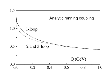
Figure 2: “Higher loop stability” of the analytic solution. The normalization point is on the $\tau$ lepton scale: $\bar{\alpha}_{s}(M_{\tau}^{2})=0.34$.

The idea that QCD running coupling can be frozen or finite at small momenta was considered in many papers (see, e.g., the discussion in Ref. [4] and interesting theoretical model in Refs. [5]). There seems to be experimental evidence in favor of such behavior. As an appropriate object, for comparison with our construction, we use the average

$$A(Q)\,=\,\frac{1}{Q}\,\int_{0}^{Q}\,dk\,{\bar{\alpha}_{s}}(k^{2})$$ (10)

that people manage to extract from jet physics data. Empirically, it has been claimed [6], [7] that this integral at $Q\simeq 1\div 2$ GeV turns out to be a fit-invariant quantity with the estimate: $A(2\,\,{\rm GeV})=0.52\pm 0.10$. Numerical results for it obtained by the substitution $\bar{\alpha}^{(2)}_{\rm an}$ into Eq. (10) with $\Lambda_{\rm an}=710\pm 110$ MeV, corresponding to $\bar{\alpha}_{\rm an}(M_{\tau}^{2})=0.36\pm 0.02$, are summarized in the Table.

$\bar{\alpha}_{\rm an}(M_{\tau}^{2})$	0.34	0.36	0.38
$\Lambda_{an}^{(2)}({\rm MeV})$	610	710	820
$A^{(2)}(2\,{\rm GeV})$	0.48	0.50	0.52

Note that a nonperturbative contribution, like the second term in the r.h.s. of Eq. (1), reveals itself even at moderate $Q$ values by “slowing down” the velocity of $\bar{\alpha}_{s}(Q)$ evolution. For instance, at $Q=3\,{\rm GeV}$ it contributes about 4%, which could be essential for the resolution of the “discrepancy” between “low-$Q$” and direct $Z_{0}$ data for $\bar{\alpha}_{s}(M_{Z})$.

As far as we have no explicit expression for the ${\bar{\alpha}_{\rm an}(Q^{2})}$ in the two-loop case, for a qualitative discussion we can use an approximate formula proposed in Ref. [3] which can be written in the form of Eq. (1) with the substitution

$$\frac{Q^{2}}{\Lambda^{2}}\to\\ \exp\left[\ln\,\frac{Q^{2}}{\Lambda^{2}}+b\ln\sqrt{\ln^{2}\,\frac{Q^{2}}{\Lambda^{2}}+4\pi^{2}}\right].$$ (11)

With appropriate redefinition of $\Lambda$, the accuracy of this approximation, for $Q\geq\Lambda$, is no less than 5%. At the same time, it produces only a 3% error in the $A(2\,{\rm GeV})$ value.

3 DISCUSSION

It is important to discuss the possibility of using ${\bar{\alpha}_{\rm an}(Q^{2})}$ in multi-prong QFT objects $\Gamma_{(k)}(s_{1},...,s_{k})$ and, particularly, in observables ${\cal M}(...Q^{2}_{i},...,q^{2}_{j}...)$ with some arguments $q^{2}_{j}=-Q^{2}_{j}>0$ being time-like (Minkowskian) and some others fixed on the mass shell.

Here, we have in mind a few different items:

1. The possibility of using RG for $k$-prong vertices $\Gamma_{(k)}(s_{1},...,s_{k})\,,k\geq 3$;

2. The technology of using ${\bar{\alpha}_{\rm an}(Q^{2})}$, originally defined for $Q^{2}_{i}>0$, in observables
   ${\cal M}(...Q^{2}_{i},...,q^{2}_{j}...)$ with time-like arguments;

3. The expediency of the ${\bar{\alpha}_{\rm an}(Q^{2})}$ continuation into the Minkowskian region $Q^{2}<0$;

4. The scheme dependence of analytic running coupling. Relation to divergencies.

Our preliminary comments on these issues are:

I. As it is well known from the old investigations, the use of RG, rigorously deduced from Dyson renormalization transformations (with finite real counterterm coefficients $z_{i}$), is justified only in the Euclidean domain and involves a simultaneous change of a scale for all arguments of $\Gamma_{(k)}(s_{j})$, i.e., $s_{j}\to s^{\prime}_{j}=ts_{j}$. This restricts the possibility of UV analysis by the so-called non-exceptional momenta.

II. Nethertheless, in some special cases it turns out to be possible to apply the RG technique to analyse multi-prong object by involving some additional means like spectral representations [8], light-cone expansion or amplitude factorization [9].

In any of above-mentioned cases the RG procedure results in solving group equations for real functions, like spectral densities and light-cone expansion coefficients. This solution involves only real running coupling ${\bar{\alpha}_{\rm an}(Q^{2})}$ values for Euclidean arguments. Any observable ${\cal M}$ with time-like value of kinematic invariant $q^{2}$ should be treated separately with an adequate procedure of analytic continuation of the observable under consideration.

III. Due to the last reason, the analytic continuation of the running coupling itself, e.g., discussing of ${\bar{\alpha}_{\rm an}(Q^{2})}$ properties in the Minkowskian region $Q^{2}<0$, in our opinion, has no direct physical meaning.

IV. The last but not least is the property of the scheme dependence of the model discussed. Formally, in our final expressions, Eqs. (6)–(9), there is no room for such dependence. This is related to the absence of UV infinities with their subtraction and renormalization ambiguities.

The analytical model has an important property. By construction it is free from UV divergencies. The log squared in the spectral function denominator (6) provides us with convergence of non-subtracted spectral representation (9). At the very end, it contains only one parameter $\Lambda$ that has to be defined from experiment. However, this needs an adequate procedure (mentioned above in the comment II) of analytization with possible liberating of infinities by contribution non-analytic in $\alpha$ for the observable confronted with data.

To summarize, it can be said that to get more satisfactory answers and, correspondingly, more complete understanding, it is necessary to continue investigation of all four issues.

Discussions

K.Chetyrkin
What do you think about an experimental testing of different predictions for the IR behavior of $\bar{\alpha}_{s}(Q)$ ?

D. Shirkov
As I showed in the Table, our model nicely correlates the $\bar{\alpha}_{s}(M_{\tau})$ measured value with the Khoze-Dokshitzer integral estimate extracted from the jet physics. This can be compared, e.g., with the $A(2\,\,{\rm GeV})$ value corresponding to the Badalian-Simonov model [5] which is of an order of 0.35.

References

- [1] D.V. Shirkov and I.L. Solovtsov, JINR Rapid Comm., No. 2[76]-96, 5, hep-ph/9604363.
- [2] N.N. Bogoliubov, A.A. Logunov and D.V. Shirkov, Sov. Phys. JETP 37(10) (1960) 574.
- [3] D.V. Shirkov and I.L. Solovtsov, hep-ph/9704363; Phys. Rev. Lett. 79 (1997) 1209.
- [4] A.C. Mattingly and P.M. Stevenson, Phys. Rev. D49 (1994) 437.
- [5] Yu.A. Simonov, Yad. Fizika, 58 (1995) 1139; A.M. Badalian and Yu.A. Simonov, ibid. 60 (1997) 714.
- [6] Yu.L. Dokshitzer and B.R. Webber, Phys. Lett. B 352 (1995) 451.
- [7] Yu.L.Dokshitzer, V.A.Khoze and S.I. Troyan, Phys. Rev. D53 (1996) 89.
- [8] I.F. Ginzburg and D.V. Shirkov, Sov. Phys. JETP 22 (1966) 234.
- [9] A.V. Efremov, A.V., Radiushkin, Riv. Nuovo Cim. 3 (1980) 1-87.