Two photon physics at LEP2

Abstract

The working group on two photon physics concentrated on three main subtopics: modelling the hadronic final state of deep inelastic scattering on a photon; unfolding the deep inelastic scattering data to obtain the photon structure function; and resonant production of exclusive final states, particularly of glueball candidates. In all three areas, new results were presented.

[Two photon physics]

• †University of Sheffield Department of Physics, Sheffield, S3 7RH. U.K.

• ‡Rutherford Appleton Laboratory, Chilton, Didcot, Oxfordshire, OX11 0QX. U.K.

• §Universität Siegen, Fachbereich Physik, D-57068 Siegen, Germany

• ¶University of Lancaster, Lancaster, LA1 4YB. U.K.

• +University College London, Gower Street, London, WC1E 6BT. U.K.

1 Introduction

Two photon physics at LEP2 is in a somewhat different position from the other topics covered in this workshop, in that the increase in beam energy makes little difference to the physics. There is a small increase in cross-section ($\propto\ln E$), but the main effect is a considerable decrease in background, because of the reduction in the annihilation cross-section. Thus, $\gamma\gamma$ physics at LEP2 is primarily an extension of work done at LEP1, but we can hope to see an improvement in our understanding as a result of larger data samples with less background contamination, and in some cases useful hardware upgrades to the experiments.

As can be seen from Professor Miller’s review[1], our present understanding of the hadronic final state in $\gamma\gamma$ interactions is not really satisfactory. The underlying physics is a complex interplay between soft (“vector dominance”) and hard (“direct”, “QPM”, “pointlike”) QCD, with the added complication of variable photon virtuality. Although in recent years a number of Monte Carlo generators for $\gamma\gamma\rightarrow\mbox{hadrons}$ have been produced[2, 3, 5], none is claimed by its authors to be applicable to the whole experimental range of $Q^{2}$, and none seems to provide a satisfactory description of the experimental data even in its claimed range of validity. The situation is doubly unfortunate because of the need to “unfold” experimental $\gamma\gamma$ data to correct for the large detector acceptance effects: if the event topology is not well reproduced by Monte Carlo, the acceptance effects are unlikely to be well modelled, and so the unfolding procedure becomes unreliable. This results in large systematic errors for one of the most important experimental measurements in $\gamma\gamma$, the photon structure function $F_{2}(x,Q^{2})$.

In view of the importance of this problem, both to $\gamma\gamma$ physics and indeed to other LEP2 analyses where $\gamma\gamma$ interactions are a significant background, the working group concentrated most of its efforts on this question of modelling the hadronic final state. Our aim was to understand where the disagreements between simulations and data arise from, and if possible to develop a prescription for ameliorating them. The results of this study are presented in section 2 of this paper. Section 3 considers in more detail the question of unfolding the photon structure function, with particular reference to the possibility of reducing systematic errors by unfolding in more than one variable. This approach relies on the fact that disagreement between Monte Carlo and data in the variable in which you unfold is not important (if it were, unfolding would be impossible, since the Monte Carlo would have to incorporate the correct distribution of the unfolded variable—which is what the unfolding is intended to discover). Therefore, if one can find a variable which characterises the difference between data and Monte Carlo and unfold in that variable as well as in $x$, the systematic errors caused by the discrepancy should be reduced.

It will be seen that both these sections are oriented towards the inclusive production of hadrons in $\gamma\gamma$ interactions, and this has indeed been the main focus of work at LEP1. However, there is now increased interest in exclusive final states, more specifically the formation of meson resonances, because of the information that can be gained on the possible glueball content of the meson so produced. Lattice gauge theory results strongly suggest that low-lying glueball states will be close in mass to conventional mesons of the same $J^{PC}$, implying that the observable states will be mixed. A meson with a high gluonium content should be suppressed in $\gamma\gamma$ production compared to gluon-rich channels such as upsilon decay and central production in hadron collisions. Admittedly LEP2 is not an ideal environment for such studies, because they impose stringent requirements on experimental triggers, but the theoretical interest is such as to warrant a feasibility study. This is considered in section 4 of this paper.

2 Modelling the hadronic final state

2.1 Introduction

The measurement of $F_{2}^{\gamma}$ in deep inelastic $e\gamma$ scattering, where only one of the electrons is “tagged” in the detector and the other one escapes unseen, involves the determination of the $\gamma^{*}\gamma$ invariant mass $W$ from the hadronic final state. Because of the non-uniform detection efficiency and incomplete angular coverage the correlation between $W_{\mathrm{v}is}$ and $W$ critically depends on the modelling of the hadronic final state. It has been shown [7] that there exist serious discrepancies in the description of this hadronic final state. Fig. 2 shows the transverse energy out of the plane, defined by the tag and the beam. For $x_{\rm vis}>0.1$ all of the generators are adequate, but for $x_{\rm vis}<0.1$ they are mutually inconsistent, and in disagreement with the data. At high $E_{\rm t,out}$ the data show a clear excess over HERWIG [2] and PYTHIA [3], while the pointlike F2GEN [8] sample exceeds the data. Similar discrepancies are observed in the hadronic energy flow per event [7], shown in Fig. 2, where both HERWIG and PYTHIA overestimate the energy in the forward region ($|\eta|>2.5$) and underestimate the energy in the central region of the detector. At $|\eta|>2$ the data are closer to the pointlike distributions from F2GEN than to the QCD models or the “perimiss” distributions of F2GEN, a mixture of peripheral and pointlike events [8]. But there is only one difference between the two F2GEN samples; the angular distribution of the outgoing quarks in the $\gamma^{\star}\gamma$ centre of mass system. This indicates that in tuning these models particular attention will need to be given to the parton distributions in the $\gamma^{\star}\gamma$ system.

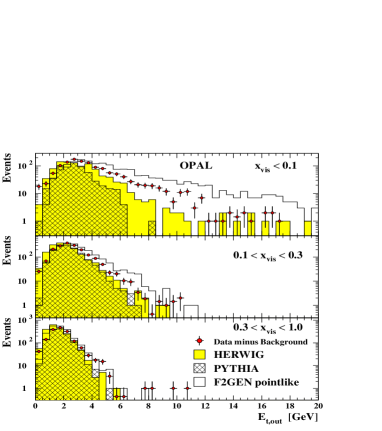
Figure 1: Transverse energy out of the tag plane, which is defined by the tag direction and beam axis.

Figure 2: Hadronic energy flow per event as a function of pseudorapidity, corrected for detector inefficiencies.

2.2 Generating hadronic final states

All the main Monte Carlo event generators for two photon physics were described in detail in the LEP2 yellow book report[9]. Little has changed since then, so we here only recap the salient features. As already mentioned, the angular distribution of the produced quarks is crucial for a good description of the data, so we concentrate on how this is generated in the different models.

2.2.1 HERWIG

In HERWIG the backward evolution algorithm is used. This means that the scattering is first set up as $\mathrm{\gamma^{*}q\to q}$, with no transverse momentum in the $\gamma\gamma^{*}$ frame. Then the history of the incoming quark is traced backwards in time to the target photon. At each step, the quark is ‘offered the chance’ to have come from a quark at higher $x$ via the emission of a gluon, $\mathrm{q\to qg}$ or directly from a pointlike photon coupling, $\mathrm{\gamma\to q\bar{q}}$. The relative probabilities of these different steps are calculated from the DGLAP evolution equation, i.e. effectively from the slopes in $x$ and $Q^{2}$ of the chosen pdf set. The evolution terminates either when a pointlike photon coupling is generated (since the pdf of photons in photons is a delta function at $x\!=\!1$), or when the evolution scale has reached the infrared cutoff $\sim 1$ GeV. In the latter case, the event is called hadronic, and in the former pointlike. Thus this separation is not made in advance but rather is generated dynamically, and depends in a non-trivial way on the evolution of the chosen set of parton distribution functions. In the ideal world, this should reproduce the assumptions made by the pdf fitters, but in practice there are many non-idealities. One finds[10] that HERWIG calls many more events hadronic than the pdf, particularly at small $x$.

This separation is of much more than passing interest, because it determines the transverse momentum distribution of the remnant (or ‘target’) quark. During this workshop, parton-level studies of several event generators were made, which found that the emission of gluons plays a relatively small rôle in determining the final state properties, and that the most important factor is the distribution of this target quark. In pointlike photon events it receives a power-law distribution according to the perturbative evolution equations, while in hadronic events it receives a Gaussian distribution of adjustable width. During the workshop we have discussed the effect of using other distributions here, and show results below.

In addition to the backward evolution, HERWIG is matched with the NLO matrix elements, which ensure that the hardest emission is distributed correctly. This effectively includes the high-$p_{t}$ photon-gluon fusion and pointlike photon processes, which can be particularly important at small $x$. They are not included in PYTHIA, which might account for the fact that HERWIG falls somewhat below the data, while PYTHIA falls precipitously in Fig. 2 for example.

2.2.2 PYTHIA/ARIADNE

PYTHIA has two options for its parton shower, either its own backward evolution algorithm, or ARIADNE’s colour dipole cascade in which there is no separation between initial-state and final-state emission. In either case it is decided in advance whether the event will be called pointlike or hadronic, and the associated distributions generated accordingly.

If PYTHIA’s own algorithm is used, then in hadronic events the backward evolution is similar to HERWIG’s described above, except that it is never evolved back to a pointlike photon, i.e. a hadronic photon is treated exactly like a hadron. The remnant is given a Gaussian transverse momentum distribution by default, although other shapes are available, as discussed below. In pointlike events, the evolution is slightly different, deciding the transverse momentum of the remnant in advance and using modified evolution equations that take that momentum into account. In common with HERWIG, this transverse momentum distribution is purely determined by perturbation theory, and there is no freedom to adjust it in the default model. During the workshop, we have tried modifying this distribution by convoluting it with a narrow (i.e. non-perturbative) Gaussian, and show results below.

If ARIADNE’s algorithm is used, the distribution of remnant momentum is the same as in PYTHIA. The evolution of the final state is modelled as being from a colour dipole between the $\mathrm{q\bar{q}}$ pair, except that the remnant quark is considered to be an extended object of size $\sim 1/p_{t}$. This means that emission in the remnant direction with $k_{\perp}\mskip 5.0mu plus 5.0mu\raisebox{-1.72218pt}{\hbox to0.0pt{$\sim$\hss}}\raisebox{1.72218pt}{$<$}\mskip 5.0mu plus 5.0mup_{t}$ is suppressed. Although ARIADNE produces significantly more gluon radiation than PYTHIA, particularly at small $x$, the fact that we have found the distribution of remnant momentum to be more important than of gluon momenta means that its predictions are not significantly different from PYTHIA’s.

2.2.3 PHOJET

PHOJET is an event generator aimed at a unified treatment of $\mathrm{pp}$, $\gamma\mathrm{p}$ and $\gamma\gamma$ collisions. It provides a very complete picture of soft effects in these collisions coupled with a somewhat less precise treatment of the perturbative evolution. It is aimed predominantly at the simulation of real photon collisions and although it generates the electron vertex keeping track of the target photon virtuality, it is only intended to be reliable for relatively low virtualities. Nevertheless, the OPAL collaboration have found that if one ignores the warnings of the authors, and runs it at higher virtualities anyway, one gets a fair description of data[11]. During this workshop, members of ALEPH have tried the same comparison and found that good agreement could only be attained by adding a vector meson form factor, and by reweighting the $x$ and $Q^{2}$ distribution by hand as described below. Having done that, we find a good description of data. One of the main features of this model relative to HERWIG and PYTHIA is the fact that it includes contributions where both photons are resolved, even for $Q^{2}$ values that would traditionally be described as deep inelastic scattering. It is possible that this is the main reason why the description of data is improved.

2.3 Studies carried out at the workshop

To study the contributions of the various partons, the PYTHIA/ARIADNE [12] energy flow in the lab frame as a function of pseudorapidity is plotted in Figure 3 for the quark that couples to the off-shell probe photon $\gamma^{\star}$, denoted the probe quark, and for the quark that couples to the quasi-real target photon $\gamma$, denoted the target quark. The total energy flow of all partons after gluon radiation is also shown. The direction of the tagged electron is always at negative $\eta$. It is apparent that the hump at negative $\eta$ stems mostly from the probe quark which is scattered in the hemisphere of the tag, while the hump at positive $\eta$ originates mostly from the target quark in the opposite hemisphere of the struck photon.

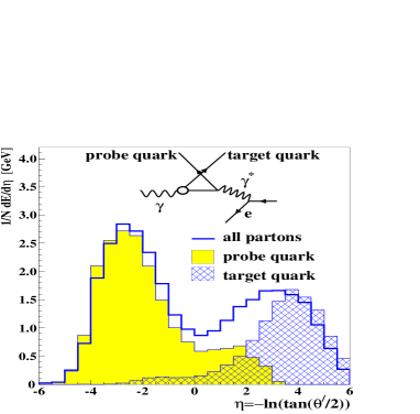
Figure 3: Energy flows of probe and target quarks.

From comparisons of the hadronic energy flow of the data with the various models, it became apparent that the energy flow of the probe quark needs to be shifted to lower $\eta$, corresponding to an increased transverse energy. This can be achieved in several ways:

Anomalous events carry more transverse momentum than hadronic events. Increasing the fraction of anomalous to hadronic or VMD type events would have the desired effect, but the pdf sets used (in this case SaS1D [13] in PYTHIA and GRV [14] in HERWIG) do not readily allow changing this ratio.

Another way to increase the transverse energy is to allow for more gluon radiation. This can be achieved by augmenting the inverse transverse size of the remnant, $\mu$, in the ARIADNE colour dipole model. In standard ARIADNE, $\mu$ is set proportional to the intrinsic $k_{T}$ of the struck quark on an event-by-event basis. For VMD events, $k_{T}$ is Gaussian with a width of 0.5 GeV. For anomalous events $k_{T}$ follows a power law. But even a generous increase of the $\mu$ parameter ($\mu=10$) has a relatively small effect on the partonic energy flow.

Increasing the intrinsic transverse momentum $k_{T}$ of the partons in the struck photon is another way of directly influencing the angular distribution of the hadronic final state. Figure 4 shows the energy flow for HERWIG events with default settings, with a fully pointlike distribution and with an enhanced $k_{T}$ distribution. Note that the run with a fully pointlike distribution looks pretty similar to the F2GEN all pointlike results, a non-trivial cross check that, in pointlike events, HERWIG seems to be behaving as expected, it is just that it is not producing enough pointlike events. As a fix, the enhanced $k_{T}$ distribution appears to be the most promising.

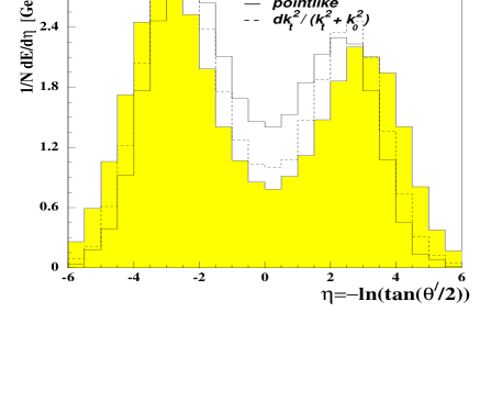
Figure 4: HERWIG energy flow of events generated with different $k_{T}$ distributions.

In PYTHIA the pdf determines whether an event is generated as a VMD or an anomalous event. The intrinsic $k_{T}$ of the quasi-real photon can be controlled with parameters [3]. Just increasing the width of the Gaussian distribution does not produce events that populate the region of high $E_{\rm t,out}$ at low $x$ observed in the data (Fig. 2). A similar deficiency had been observed in the resolved photoproduction data at ZEUS [16], which led to the introduction of a power-like $k_{T}$-distribution of the form $dk_{T}^{2}/(k_{T}^{2}+k_{0}^{2})$, improving the distributions of the photon remnant. The parameter $k_{0}$ is a constant, set to 0.66 GeV in [16]. The PYTHIA parameters only allow adjusting the $k_{T}$ for VMD type events, figure 5, but not for anomalous evens. To change the intrinsic $k_{T}$ of anomalous events a Gaussian smearing is added in quadrature [15].

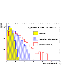
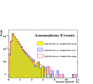
Figure 5: Transverse momentum of the target quark in PYTHIA/ARIADNE for VMD and anomalous events.

2.4 Comparisons of models with data

Figure 7 show the $E_{\rm t,out}$ and figure 9 the hadronic energy flows on detector level of PYTHIA with default parameter settings and with the $dk_{T}^{2}/(k_{T}^{2}+k_{0}^{2})$ distribution for VMD plus a Gaussian smearing of the anomalous events, compared to the OPAL data taken in 1993–1995 at $\sqrt{s_{ee}}=91$ GeV [17]. In addition the ARIADNE distributions with enhanced gluon radiation are shown. While the $E_{\rm t,out}$ spectrum has been improved, it still falls short of the data in the tail of the distribution. The hadronic energy flow generated by the enhanced PYTHIA recreates the peak on the remnant side (positive $\eta$) seen in the data at low $x_{\rm vis}$, at the expense of a somewhat worse fit on the tag side.

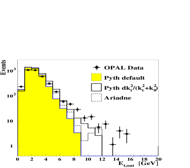
Figure 6: PYTHIA: Transverse energy out of the tag plane.

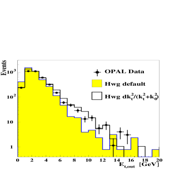
Figure 7: HERWIG: Transverse energy out of the tag plane.

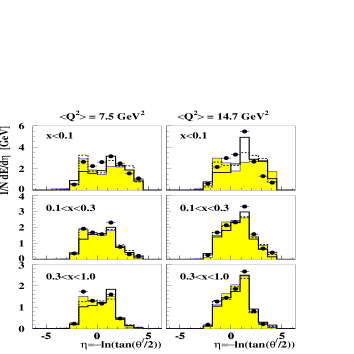
Figure 8: PYTHIA: Hadronic energy flow as function of $x$ and $Q^{2}$. The symbols are the same as in Fig. 6

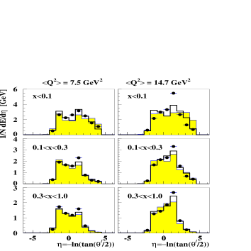
Figure 9: HERWIG: Hadronic energy flow as function of $x$ and $Q^{2}$. The symbols are the same as in Fig. 7

HERWIG separates events dynamically into hadronic and anomalous type. A similar $dk_{T}^{2}/(k_{T}^{2}+k_{0}^{2})$ distribution of the intrinsic transverse momentum of hadronic photons can be added by hand. The results of this are shown in figures 7 and 9. Both the $E_{\rm t,out}$ and the energy flows are greatly improved with the inclusion of the power-like $k_{T}$ distribution, with the exception of the peak in the energy flow at low $x_{\rm vis}$ – high $Q^{2}$, which still falls short of the data.

A similar improvement is also seen in the description of ALEPH data[18], as seen in figures 11 and 11. In these plots the average $Q^{2}$ is 14.2 $\mbox{GeV}^{2}$ and the full $x$ range is integrated over.

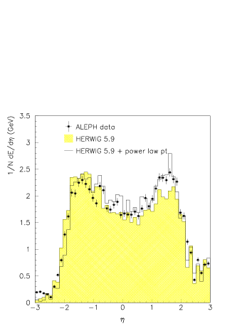
Figure 10: Hadronic energy flow: HERWIG vs. ALEPH.

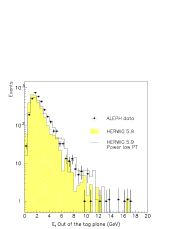
Figure 11: Transverse energy out of the tag plane: HERWIG vs. ALEPH.

Overall, the power-like distribution of the intrinsic transverse momentum of the struck photon of the form $dk_{T}^{2}/(k_{T}^{2}+k_{0}^{2})$ greatly improves the hadronic final state distributions of both PYTHIA and HERWIG. This improved description of the data should reduce the model-dependent systematic errors in the unfolded result of the photon structure function $F_{2}^{\gamma}$. More fine-tuning of these models is required.

A number of LEP experiments have observed that the PHOJET program provides the best available description of real photon interactions as observed in untagged events. Despite this being expressly forbidden by the author of the program, it has also been compared to tagged events by OPAL and found to give an acceptable description of their data[11]. At the workshop this was attempted for the first time using ALEPH tagged data.

The event selection is described in Ref. [19]. The ALEPH version of PHOJET was adapted to produce tagged events with a Generalized Vector Dominance form factor. A comparison of the model to the data is given in figures 12 and 13. The dashed lines in these distributions show the PHOJET distributions that resulted. In some of the distributions the agreement between data and Monte Carlo is better than that achieved by existing models. However the $x_{vis}$ distribution shows the Monte Carlo exceeding the data at low $x_{vis}$ which suggest that the $x_{true}$ distribution is also too strongly peaked at low values. This could also cause the disagreement in the $W_{vis}$ and $Q^{2}$ distributions. In order to test this the true $x$ distribution was compared for PHOJET and HERWIG using the GRV structure function as input. This version of HERWIG gives a good description of the ALEPH $x_{vis}$ distribution in this $Q^{2}$ region. The ratio of these two $x_{true}$ distributions was obtained and parameterised with a fourth degree polynomial. This function was then used to weight the events in the histogram. This is shown by the solid line in figure 12 and results in a better fit to the data in the variables considered here than the models currently used in ALEPH.

Figure 12: Comparison of PHOJET to the data. The data are shown by the points with error bars. The histograms are the sum of the PHOJET and $\gamma\gamma\rightarrow\tau^{+}\tau^{-}$ models. The PHOJET model has been normalised to the data. The solid line is the result after reweighting the events to obtain the same $x_{true}$ distribution as is found in HERWIG with GRV input structure function. The dashed line is the Monte Carlo data before this weighting has been applied.

As we have seen several times at this workshop, the models currently used in tagged $\gamma^{*}\gamma$ studies do not describe the data when considered in terms of the pseudorapidity $\eta$ and and the azimuthal separation $\phi_{sep}$. Fig. 13 shows these distributions for the ALEPH data compared to the Monte Carlo events. It can be seen that the tagged PHOJET model does a better job of fitting the data than does HERWIG, and this improvement is even greater once the reweighting has been applied.

Figure 13: Energy flow as a function of (a) $\phi_{\mathrm{sep}}\,$, (b) $\eta$. The points are the data. Solid line: HERWIG with GRV; dotted line: PHOJET; dashed line: reweighted PHOJET.

2.5 Summary and conclusions

It is becoming steadily clearer and clearer that the data show a much more pointlike structure than the QCD-inspired Monte Carlo models. In order to provide reliable unfolding of the structure function $F_{2}$, it is essential to have theoretically well-founded models that are capable of giving good fits to data after variation in $F_{2}$. We do not have any models that fulfil both criteria at present. They must be well-founded, because we must know that the $x_{\mathrm{vis}}$ distribution extracted is somehow related to that predicted theoretically. They must be able to give a good fit to data, otherwise we will not believe the unfolding procedure at all. One way out of this situation is to unfold in several additional variables simultaneously, thereby unfolding away the model-dependence, as discussed in the next section. Another is clearly to improve the models until they do fulfil the criteria.

While we have come no closer to finding a theoretically-sound model that describes data well, we have made progress in finding models that are able to give a good description of data at all. Unfortunately this has meant poorly-motivated modifications in each case: in PYTHIA we have added Gaussian intrinsic transverse momentum to anomalous events; in HERWIG we have added power-like transverse momentum to hadronic events; and we have used PHOJET in regions for which it should not be valid.

We should not however be entirely negative about these modifications. Two photon physics is not out on its own, but is closely related to other areas of particle physics, particularly those being studied at HERA, proton DIS and photoproduction. Similar problems are being found there – too little transverse momentum in the proton direction in DIS and in the photon remnant direction in photoproduction. We can therefore draw some phenomenological satisfaction from the fact that the same solutions seem to work in both cases, like including a power-like photon remnant transverse momentum distribution and a resolved component in DIS.

3 Unfolding the photon structure function

The large integrated luminosity expected from the LEP II programme will provide new opportunities to investigate $\gamma\gamma$ collisions. Single-tag events, where one electron remains in the beam pipe and the other is measured with an angle $\theta_{\rm tag}$ and energy $E_{\rm tag}$, can be viewed as the deep inelastic scattering of an electron and an (almost) real target photon. Of particular interest is the joint distribution of the negative four-momentum squared of the probing photon, $Q^{2}=4E_{\rm tag}E_{\rm beam}\sin^{2}(\theta_{\rm tag}/2)$, and the invariant mass of the hadronic system, $W$. Equivalently, one usually measures the distribution $Q^{2}$ and the variable $x=Q^{2}/(Q^{2}+W^{2})$; this can be directly related to the photon structure function $F_{2}^{\gamma}(x,Q^{2})$. (The formalism of single-tag $\gamma\gamma$ collisions is described in e.g. [21]). In this paper we concentrate on the question of measuring the distribution of $x$ for single-tag $\gamma\gamma$ collisions within a given narrow range of $Q^{2}$.

The dominant uncertainties in current measurements of the $x$ distribution are related to corrections that must be introduced to account for finite acceptance and resolution of the detector. These effects stem mainly from hadrons at low angles with respect to the beam line that escape detection. This results in a lower measured hadronic mass compared to its true value, and hence in a corresponding distortion of the variable $x$. This is in contrast to the situation with $Q^{2}$, which is entirely determined by the tag electron’s angle and energy. It can therefore be measured to within several percent, and corrections for resolution effects do not pose a major problem. Here we will concentrate on unfolding the distribution of $x$.

A detailed description of unfolding problems can be found in [22]. We can represent a sample of measured values of $x$ by means of a histogram with $M$ bins. The expectation values of the numbers of events $\mathchoice{\mbox{\boldmath$\displaystyle\bf\mu$}}{\mbox{\boldmath$\textstyle\bf\mu$}}{\mbox{\boldmath$\scriptstyle\bf\mu$}}{\mbox{\boldmath$\scriptscriptstyle\bf\mu$}}=(\mu_{1},\ldots,\mu_{M})$ that would be obtained with a perfect detector are thus the parameters which we want to estimate. What we obtain from the experiment is a histogram $\mathchoice{\mbox{\boldmath$\displaystyle\bf n$}}{\mbox{\boldmath$\textstyle\bf n$}}{\mbox{\boldmath$\scriptstyle\bf n$}}{\mbox{\boldmath$\scriptscriptstyle\bf n$}}=(n_{1},\ldots,n_{N})$, which is distorted with respect to $\textstyle\bf\mu$ both because of statistical fluctuations as well as from the effects of acceptance and resolution. The latter can cause an event with a true value of $x$ in bin $i$ to be observed in some different bin $j$. (Note that in general the $M$ bins for the true histogram $\textstyle\bf\mu$ need not be the same as the $N$ bins of the observed histogram $\textstyle\bf n$. In the following, however, we will use the same binning for both.)

The number of entries $n_{i}$ observed in a given bin $i$ can be treated as a Poisson variable with expectation value $\nu_{i}=E[n_{i}]$. The vectors $\textstyle\bf\mu$ and $\textstyle\bf\nu$ are related by

$$\mathchoice{\mbox{\boldmath$\displaystyle\bf\nu$}}{\mbox{\boldmath$\textstyle\bf\nu$}}{\mbox{\boldmath$\scriptstyle\bf\nu$}}{\mbox{\boldmath$\scriptscriptstyle\bf\nu$}}=R\mathchoice{\mbox{\boldmath$\displaystyle\bf\mu$}}{\mbox{\boldmath$\textstyle\bf\mu$}}{\mbox{\boldmath$\scriptstyle\bf\mu$}}{\mbox{\boldmath$\scriptscriptstyle\bf\mu$}}\,+\,\mathchoice{\mbox{\boldmath$\displaystyle\bf\beta$}}{\mbox{\boldmath$\textstyle\bf\beta$}}{\mbox{\boldmath$\scriptstyle\bf\beta$}}{\mbox{\boldmath$\scriptscriptstyle\bf\beta$}}\>,$$ (1)

where the matrix element $R_{ij}$ represents the probability for an event to be observed in bin $i$ given that its true $x$ value was in bin $j$, and the vector $\mathchoice{\mbox{\boldmath$\displaystyle\bf\beta$}}{\mbox{\boldmath$\textstyle\bf\beta$}}{\mbox{\boldmath$\scriptstyle\bf\beta$}}{\mbox{\boldmath$\scriptscriptstyle\bf\beta$}}=(\beta_{1},\ldots,\beta_{N})$ gives the expected background. Here for simplicity we will neglect the background, and thus equation (1) becomes $\mathchoice{\mbox{\boldmath$\displaystyle\bf\nu$}}{\mbox{\boldmath$\textstyle\bf\nu$}}{\mbox{\boldmath$\scriptstyle\bf\nu$}}{\mbox{\boldmath$\scriptscriptstyle\bf\nu$}}=R\mathchoice{\mbox{\boldmath$\displaystyle\bf\mu$}}{\mbox{\boldmath$\textstyle\bf\mu$}}{\mbox{\boldmath$\scriptstyle\bf\mu$}}{\mbox{\boldmath$\scriptscriptstyle\bf\mu$}}$. Note that a true value in bin $j$ need not lead to any measured value at all, i.e. the efficiencies

$$\varepsilon_{j}=\sum_{i=1}^{N}R_{ij}$$ (2)

are in general less than unity.

If we had the vector $\textstyle\bf\nu$, then we could simply invert $R$ to obtain $\mathchoice{\mbox{\boldmath$\displaystyle\bf\mu$}}{\mbox{\boldmath$\textstyle\bf\mu$}}{\mbox{\boldmath$\scriptstyle\bf\mu$}}{\mbox{\boldmath$\scriptscriptstyle\bf\mu$}}=R^{-1}\mathchoice{\mbox{\boldmath$\displaystyle\bf\nu$}}{\mbox{\boldmath$\textstyle\bf\nu$}}{\mbox{\boldmath$\scriptstyle\bf\nu$}}{\mbox{\boldmath$\scriptscriptstyle\bf\nu$}}$. What we have instead, however, are the data values $\textstyle\bf n$, which are subject to random fluctuations. The estimators $\mathchoice{\mbox{\boldmath$\displaystyle\bf\hat{\mu}$}}{\mbox{\boldmath$\textstyle\bf\hat{\mu}$}}{\mbox{\boldmath$\scriptstyle\bf\hat{\mu}$}}{\mbox{\boldmath$\scriptscriptstyle\bf\hat{\mu}$}}=R^{-1}\mathchoice{\mbox{\boldmath$\displaystyle\bf n$}}{\mbox{\boldmath$\textstyle\bf n$}}{\mbox{\boldmath$\scriptstyle\bf n$}}{\mbox{\boldmath$\scriptscriptstyle\bf n$}}$ are unbiased, but have extremely large variances. (In the following, estimators will be denoted by hats.) These are in fact the estimators that one obtains by maximizing the log-likelihood function based on Poisson-distributed data,

$$\log L(\mathchoice{\mbox{\boldmath$\displaystyle\bf\mu$}}{\mbox{\boldmath$\textstyle\bf\mu$}}{\mbox{\boldmath$\scriptstyle\bf\mu$}}{\mbox{\boldmath$\scriptscriptstyle\bf\mu$}})=\sum_{i=1}^{N}\log\left(\frac{\nu_{i}^{n_{i}}}{n_{i}!}\,e^{-\nu_{i}}\right)\>,$$ (3)

which becomes

$$\log L(\mathchoice{\mbox{\boldmath$\displaystyle\bf\mu$}}{\mbox{\boldmath$\textstyle\bf\mu$}}{\mbox{\boldmath$\scriptstyle\bf\mu$}}{\mbox{\boldmath$\scriptscriptstyle\bf\mu$}})=\sum_{i=1}^{N}(n_{i}\log\nu_{i}-\nu_{i})$$ (4)

after dropping terms not depending on the parameters. (Note that this is regarded as a function of $\textstyle\bf\mu$, since one has $\mathchoice{\mbox{\boldmath$\displaystyle\bf\nu$}}{\mbox{\boldmath$\textstyle\bf\nu$}}{\mbox{\boldmath$\scriptstyle\bf\nu$}}{\mbox{\boldmath$\scriptscriptstyle\bf\nu$}}=R\mathchoice{\mbox{\boldmath$\displaystyle\bf\mu$}}{\mbox{\boldmath$\textstyle\bf\mu$}}{\mbox{\boldmath$\scriptstyle\bf\mu$}}{\mbox{\boldmath$\scriptscriptstyle\bf\mu$}}$.)

The idea behind unfolding is to construct estimators $\textstyle\bf\hat{\mu}$ with much smaller variances than the maximum likelihood estimators, at the cost of introducing a small bias. In regularized unfolding, this is done by choosing the smoothest solution (according to some criterion) out of those for which the log-likelihood is within some $\Delta\log L$ of its maximum value. This is equivalent to maximizing a linear combination of $\log L(\mathchoice{\mbox{\boldmath$\displaystyle\bf\mu$}}{\mbox{\boldmath$\textstyle\bf\mu$}}{\mbox{\boldmath$\scriptstyle\bf\mu$}}{\mbox{\boldmath$\scriptscriptstyle\bf\mu$}})$ and a regularization function $S(\mathchoice{\mbox{\boldmath$\displaystyle\bf\mu$}}{\mbox{\boldmath$\textstyle\bf\mu$}}{\mbox{\boldmath$\scriptstyle\bf\mu$}}{\mbox{\boldmath$\scriptscriptstyle\bf\mu$}})$,

$$\varphi(\mathchoice{\mbox{\boldmath$\displaystyle\bf\mu$}}{\mbox{\boldmath$\textstyle\bf\mu$}}{\mbox{\boldmath$\scriptstyle\bf\mu$}}{\mbox{\boldmath$\scriptscriptstyle\bf\mu$}},\lambda)=\alpha\log L(\mathchoice{\mbox{\boldmath$\displaystyle\bf\mu$}}{\mbox{\boldmath$\textstyle\bf\mu$}}{\mbox{\boldmath$\scriptstyle\bf\mu$}}{\mbox{\boldmath$\scriptscriptstyle\bf\mu$}})\,+\,S(\mathchoice{\mbox{\boldmath$\displaystyle\bf\mu$}}{\mbox{\boldmath$\textstyle\bf\mu$}}{\mbox{\boldmath$\scriptstyle\bf\mu$}}{\mbox{\boldmath$\scriptscriptstyle\bf\mu$}})\,+\,\lambda\left[n_{\rm tot}\,-\,\sum_{i=1}^{N}\nu_{i}\right]\>,$$ (5)

with respect to the parameters $\textstyle\bf\mu$ and the Lagrange multiplier $\lambda$. The function $S(\mathchoice{\mbox{\boldmath$\displaystyle\bf\mu$}}{\mbox{\boldmath$\textstyle\bf\mu$}}{\mbox{\boldmath$\scriptstyle\bf\mu$}}{\mbox{\boldmath$\scriptscriptstyle\bf\mu$}})$ must be defined to reflect the smoothness of the solution. The regularization parameter $\alpha$ determines the trade-off between likelihood and smoothness, and can be chosen to correspond to a given value of $\Delta\log L=\log L_{\rm max}-\log L(\mathchoice{\mbox{\boldmath$\displaystyle\bf\mu$}}{\mbox{\boldmath$\textstyle\bf\mu$}}{\mbox{\boldmath$\scriptstyle\bf\mu$}}{\mbox{\boldmath$\scriptscriptstyle\bf\mu$}})$. The final term in $\varphi$ restricts the solution to satisfy $\sum_{i}\nu_{i}=\sum_{i,j}R_{ij}\mu_{j}=n_{\rm tot}$, where $n_{\rm tot}$ is the total number of events observed.

A commonly used regularization function is based on the mean squared second derivative of the unfolded distribution (Tikhonov regularization). Computer programs based on this technique have been used in previous structure function measurements [23, 24]. The regularization function can be implemented by approximating the second derivative of the distribution using finite differences. This leads to a function of the form

$$S(\mathchoice{\mbox{\boldmath$\displaystyle\bf\mu$}}{\mbox{\boldmath$\textstyle\bf\mu$}}{\mbox{\boldmath$\scriptstyle\bf\mu$}}{\mbox{\boldmath$\scriptscriptstyle\bf\mu$}})=-\sum_{i,j=1}^{M}G_{ij}\,\mu_{i}\,\mu_{j}\>,$$ (6)

where coefficients $G_{ij}$ must be determined so as to take into account differences in the bin widths; cf. [22]. Another possible regularization function is

$$S(\mathchoice{\mbox{\boldmath$\displaystyle\bf\mu$}}{\mbox{\boldmath$\textstyle\bf\mu$}}{\mbox{\boldmath$\scriptstyle\bf\mu$}}{\mbox{\boldmath$\scriptscriptstyle\bf\mu$}})=-\sum_{j=1}^{M}\mu_{j}\log\frac{\mu_{j}}{\mu_{\rm tot}}=-\mu_{\rm tot}\sum_{j=1}^{M}p_{j}\log p_{j}=\mu_{\rm tot}H\>,$$ (7)

where $\mu_{\rm tot}=\sum_{i=1}^{M}\mu_{i}$, $p_{j}=\mu_{j}/\mu_{\rm tot}$, and $H$ is the Shannon entropy. The entropy-based regularization function makes no reference to the relative locations of any of the bins, which has the advantage that the bins at the edges of the distribution are treated on the same footing as those in the middle. In addition, use of (7) (referred to in the following as MaxEnt) can be directly applied to multidimensional distributions.

One can show that the estimators $\textstyle\bf\hat{\mu}$ obtained from any regularized unfolding technique are biased. An additional systematic error is related to the model dependence of the response matrix $R$. This matrix must in general be determined by a Monte Carlo calculation where events are generated and processed by a detector simulation program. By construction, the conditional probability for an event to be observed at $x^{\prime}$ given that it was generated at $x$ is independent of the distribution of $x$. The corresponding statement for finite bins in $x$ is approximately true as long as the bins are not too large.

The true value of $x$ is not, however, the only variable that has an influence on the probability to measure a given value $x^{\prime}$. For example, if the hadrons are mostly at low angles with respect to the beam line, then the resolution for $x$ will be poor, since on average more particles will be lost. Since different models have in general different distributions for all of the variables that characterize the final state hadrons, each will lead to somewhat different response matrices $R$, and hence to different results for the unfolded $x$ distribution.

A method to reduce this model dependence is to measure for each event not only $x$, but in addition some other variable $y$ (to be defined) that also characterizes the final state. The response matrix gives the probability for an event with true values of $x$ and $y$ in bins $i$ and $j$ to be observed in bins $k$ and $l$. This matrix is now by construction independent of the model’s joint distribution of $x$ and $y$. In principle this idea could be extended to an arbitrary number of additional variables, and eventually one would eliminate all model dependence from the response matrix. Since the individual cells of the multidimensional space must be populated with enough Monte Carlo events to determine the response matrix, however, the total number of bins, and hence the number of variables, is necessarily limited. Here we will only consider the case of two measured variables.

In order to reduce the model dependence of $R$, the second variable $y$ should be related to the detector’s ability to measure $x$. Here, we consider $y=|\cos\theta_{\rm had}|$, where $\theta_{\rm had}$ is the polar angle of the total hadronic system in the laboratory frame. In fact, large discrepancies between observed and predicted angular distributions of hadrons have been observed in single-tag events [25]. Thus some reduction in the uncertainty from model dependence can be expected by obtaining this information directly from the data. Other possibilities are the orientation of the hadronic system with respect to the $\gamma\gamma$ axis, or a quantity related to hard gluon radiation, such as the thrust or jet structure of the hadrons measured in the $\gamma\gamma$ rest frame. After unfolding the distribution of $x$ and $|\cos\theta_{\rm had}|$, we will integrate over $|\cos\theta_{\rm had}|$ to obtain the distribution of $x$ alone.

In order to investigate these ideas quantitatively, single-tag $\gamma\gamma$ events were generated with the HERWIG Monte Carlo generator [2]. This allows the user to choose from a variety of parametrizations for the photon structure function from the package PDFLIB [26].

The response matrix was determined by means of a highly simplified detector simulation program, roughly corresponding to a typical LEP detector. An electromagnetic calorimeter was assumed to be sensitive to photons and electrons with energies $E>200$ MeV, to be hermetic down to 30 mrad from the beam line, and was taken to have an energy resolution of $\sigma_{E}=0.18\sqrt{E}$. A hadron calorimeter in the angular range $|\cos\theta|<0.99$ was assumed to be fully efficient for energies above 1.0 GeV, and to have an energy resolution of $\sigma_{E}=0.80\sqrt{E}$. Charged particles with $|\cos\theta|<0.94$ and transverse momentum $p_{\perp}>150$ MeV are measured with a resolution of $\sigma_{p_{\perp}}/p_{\perp}=0.003\oplus 0.0008\cdot p_{\perp}$. It was assumed that electrons with energies of at least 10 GeV and $\theta>30$ mrad could be identified.

First, large samples of single-tag events (approximately 12 fb^-1) were generated at a centre-of-mass energy of $E_{\rm cm}=184$ GeV with HERWIG using the GRV LO [14], SaS1D [13] and LAC1 [27] structure functions. True single-tag events were defined to be those with a tag electron in the range $60<\theta<100$ mrad, which for the GRV structure functions gives a mean $Q^{2}$ of 40.0 GeV² and a cross section of 11.6 pb. These events were processed by the detector simulation routine in order to determine a response matrix $R$ based on each of the three sets of structure functions.

Scatter plots of the true and observed values of $x$ are shown in Fig. 14 for two different ranges of $|\cos\theta_{\rm had}|$. In Fig. 14(a), the (true) hadronic system has an angle of at least 60^∘ with the beam line. This results in a relatively good measurement of the hadronic mass $W$, and hence in a good resolution for $x$. In Fig. 14(b), the hadronic system has $|\cos\theta_{\rm had}|>0.9$, so that a larger fraction of the hadrons escape detection. This leads to a visibly weaker correlation between the measured and true values of $x$.

The effect of the direction of the hadronic system on the $x$ resolution can also be seen in Fig. 15, showing (a) the mean and (b) the standard deviation $\sigma_{x}$ of $x_{\rm vis}$ as a function of $x_{\rm true}$ for the same ranges of $\cos\theta_{\rm had}$ as in Fig. 14. For $x$ less than around 0.3, the typical $x$ resolution is between 0.12 and 0.18 for $|\cos\theta_{\rm had}|>0.9$, but is around 0.08 – 0.13 for $|\cos\theta_{\rm had}|<0.5$. Thus if two models differ in their distributions of $\cos\theta_{\rm had}$, they will result in different response matrices for $x$.

In order to minimize the errors in the unfolded result, the bin size should not be too much smaller than the resolution. The bins should be sufficiently small, however, so that the resolution is approximately constant over a bin. At low $x$, these two considerations come into conflict. The bin boundaries for $x$ were chosen to be $[0.0,0.05,0.1,0.2,0.3,0.4,0.6,0.8,1.0]$ (8 bins). The resolution for $|\cos\theta_{\rm had}|$ is around 0.20 – 0.25 for $|\cos\theta_{\rm had}|<0.5$, and improves to around 0.18 as $|\cos\theta_{\rm had}|$ increases. The bins for $|\cos\theta_{\rm had}|$ were chosen to be $[0.0,0.3,0.5,0.7,0.8,0.9,1.0]$ (6 bins).

To test the unfolding procedure, a smaller independent sample of events was generated using the GRV structure functions and processed by the detector simulation routine; the resulting events were treated as real data. The test sample corresponds to 207 pb^-1, and consists of 2444 true single-tag events (according to the definition above). Of these, 1697 passed relatively loose event selection criteria, having a tag electron measured in the range $60<\theta<100$ mrad, no electron on the opposite side above 30 mrad, and in addition, at least three charged particle tracks.

Figure 16(a) shows the distribution $dN/dx$ based on large samples of data generated with the GRV, SaS1D and LAC1 structure functions, normalized to the expected number of entries for an integrated luminosity of 207 pb^-1. Figure 16(b) shows the GRV predicted distribution of $x_{\rm true}$, $dN_{i}/dx=\mu_{i}/\Delta x_{i}$, where $\Delta x_{i}$ is the width of bin $i$. Also shown are the expectation values of what one would observe including the effects of detector acceptance and resolution, corresponding to the histogram $\textstyle\bf\nu$. The histogram of $x_{\rm vis}$ from the simulated data, i.e. the vector $\textstyle\bf n$ divided by the bin widths, is shown as points with error bars. These are subject to both detector effects and statistical fluctuations.

First, the difference between Tikhonov and MaxEnt regularization was investigated using the test data sample and response matrix both based on GRV. Figure 17 shows the result of a one-dimensional unfolding of the $x$ distribution, with statistical error bars, using (a) Tikhonov and (b) entropy-based regularization functions. The regularization parameter $\alpha$ was determined in both cases such that the biases of the estimators, $b_{i}=E[\hat{\mu}_{i}]-\mu_{i}$, are consistent with zero within their own statistical errors. This is done by constructing estimators $\hat{b}_{i}$ for the biases; cf. [22]. Here this criterion leads to larger errors for the MaxEnt case. Because of this fact, however, MaxEnt gives a better level of agreement between the estimated and true distributions within the statistical errors. The bias in the Tikhonov result can be reduced by increasing the regularization parameter, in which case it becomes similar to that shown here from MaxEnt. The prescription for setting $\alpha$ is by no means unique, and a corresponding systematic uncertainty should be assigned to the final result. A reasonable measure of this uncertainty is given by the estimated bias.

Next, the question of model dependence of the response matrix was investigated using MaxEnt regularization. Figure 18(a) shows results obtained using response matrices from HERWIG with GRV, SaS1D and LAC1 structure functions, where the test data sample was in all three cases based on GRV. All of the results are in reasonable agreement with the true values within their statistical errors. From the ratio of unfolded to true distributions in Fig. 18(b), one can see that the unfolded result indeed depends on which response matrix is used.

Figure 19 shows the result of a two-dimensional unfolding of the variables $x$ and $|\cos\theta_{\rm had}|$, again using the entropy-based regularization function, and the same criterion as before for determining the regularization parameter. Again, all of the results are in reasonable agreement with the true values within the statistical errors. Here, however, the spread between the points for different models is reduced with respect to what was obtained from the one-dimensional unfolding. The differences between results from GRV and SaS1D matrices differ by 1 – 5%, except for a 9% change for the second bin; these shifts are much smaller than the relative statistical errors of the unfolded $\hat{\mu}_{i}$.

It is not entirely clear why the entropy-based regularization gives smaller statistical errors in the two-dimensional case than when unfolding in one dimension. Although the variable $\cos\theta_{\rm had}$ should reduce the model dependence of the response matrix, $x$ and $\cos\theta_{\rm had}$ are only weakly correlated, and hence the angle of the hadronic system does not directly provide information about $x$. It appears here that the prescription for determining the regularization parameter led to a solution with smaller errors in the two-dimensional case. It is not obvious whether this is particular to the example done here, or rather is true more generally.

Although some improvement with two-dimensional unfolding was anticipated, the exact reasons for the differences between the one and two-dimensional cases here are not yet fully understood. A large reduction in model dependence would be expected if the models had very different distributions of $\cos\theta_{\rm had}$. This distribution does not change much, however, when the HERWIG model is used with different structure functions, and hence the three models considered here are not very different in this regard. Further investigation with other models in which the $\cos\theta_{\rm had}$ distributions show greater differences will indicate whether the two-dimensional procedure in fact gives a significant improvement in the result.

4 Exclusive final states

In this section we discuss exclusive reactions of the type

$$\gamma\gamma\to n\mbox{~{}hadrons},$$ (8)

where $n$ is small, 2, 3 or 4. In particular, we focus on the case of resonant production of a single hadronic state, $X$,

$$\gamma\gamma\to X\to n\mbox{~{}hadrons}.$$ (9)

This provides a direct measurement of the two-photon width of the state $X$, $\Gamma(X\to\gamma\gamma)$, which is an important input to the understanding of meson spectroscopy, as we discuss in section 4.1. In section 4.2 we discuss the extent to which such measurements might be made at LEP2.

4.1 Motivation

Two photon collisions provide a sensitive flavour-dependent probe of the $\mathrm{q\bar{q}}$ spectrum. It is important to establish the spectroscopy of the 1–2.5 GeV region, where many of the assignments that have been made are only tentative. One of the most important questions in the strongly-interacting limit of QCD is whether or not purely gluonic bound states exist.

In recent years lattice QCD calculations have improved enormously in precision. The systematic errors are under good control, and several different calculations come to the same conclusion: that the lowest lying gluonic state has $J^{PC}=0^{++}$ and a mass of

$$m_{G}=1.61\pm 0.07\pm 0.13\mskip 5.0mu plus 5.0mu\mathrm{GeV},$$ (10)

where the first error is statistical and the second is a systematic error estimated from the remaining discrepancies between different calculations[28]. There is also evidence that the $2^{++}$ and $0^{-+}$ states lie around 2 GeV, although here the calculations have considerably larger uncertainties. Lattice calculations also give us the width of the $0^{++}$ decay to pseudoscalars,

$$\Gamma_{G}\sim 100\mskip 5.0mu plus 5.0mu\mathrm{MeV},$$ (11)

although again with considerable uncertainty.

Not surprisingly, one expects glueballs to be produced most easily in gluon-rich environments. The classic example is of $J/\psi$ radiative decays, in which the lowest-order perturbative contribution is

$$J/\psi\to\gamma\,g\,g,$$ (12)

where the gluon pair must be in a colour-singlet state, since both the $J/\psi$ and photon are colour singlets. Thus this is ready to be projected directly on to a glueball wave function. Comparing this with the production of a normal meson, in which the gluons must first annihilate to a $q\bar{q}$ pair, which are then projected on to the meson wave function, we can estimate

$$\frac{\Gamma(J/\psi\to\gamma G)}{\Gamma(J/\psi\to\gamma M)}\sim\frac{1}{\alpha_{s}^{2}}.$$ (13)

The exact opposite is true in two photon collisions, which are quark-rich environments. A glueball can only be produced via the annihilation of a $q\bar{q}$ pair into a pair of gluons, whereas a normal meson can be produced directly, so we can estimate

$$\frac{\sigma(\gamma\gamma\to M)}{\sigma(\gamma\gamma\to G)}=\frac{\Gamma(M\to\gamma\gamma)}{\Gamma(G\to\gamma\gamma)}\sim\frac{1}{\alpha_{s}^{2}}.$$ (14)

The stickiness of a mesonic state is defined as

$$S_{X}=\frac{\Gamma(J/\psi\to\gamma X)}{\Gamma(X\to\gamma\gamma)}.$$ (15)

We expect the stickiness of all normal mesons to be comparable, while for glueballs, we expect it to be enhanced, from the above arguments, by a factor

$$\frac{S_{G}}{S_{M}}\sim\frac{1}{\alpha_{s}^{4}}.$$ (16)

Bearing in mind that this $\alpha_{s}$ refers to a very low momentum-transfer process, we should estimate $\alpha_{s}\sim\frac{1}{2}$, and hence $S_{G}/S_{M}\sim 20$.

Measuring the two-photon cross section has always therefore been considered a classic test of the nature of a putative glueball.

Glueball phenomenology has recently been revolutionized by the realization that the glueball is likely to mix significantly with other $0^{++}$ mesons. In particular, if it has mass $\sim 1600$ MeV, it should lie in the middle of a multiplet whose light $I\!\!=\!\!0$ member is the $f_{0}(1370)$ and which is expected to have a hidden-strange member at around 1600–1700 MeV. Because of this mixing, many of the classic phenomenological differences between glueballs and normal mesons will be reduced. For example the stickiness of a mixed glueball-normal meson should be between those of pure glueball and pure non-glueball states. Since the wave function of a mixed state can be estimated as

$$|G\rangle=|G_{0}\rangle+\sum|Q\rangle\frac{\langle Q|H_{I}|G\rangle}{E_{Q}-E_{G}},$$ (17)

the precise properties of the mixed states are strongly dependent on where in the multiplet the gluonic state lies, i.e. on the energy difference $E_{Q}\!-\!E_{G}$.

The Crystal Barrel experiment have observed two mesons with unusual properties in exactly the region one expects mixed glueball and hidden strange states:

$$\begin{array}[]{ccc}J=&0&0\mbox{~{}or~{}}2,\\ m=&1.50&1.71,\\ \Gamma=&120\pm 20&140\pm 12.\end{array}$$ (18)

In particular, attention has focused on the 1500 state as the most promising glueball candidate we have. It has unusual decays, being about 50% to $4\pi$, apparently more through $\sigma\sigma$ than $\rho\rho$, and with the $\eta\eta$ and even $\eta\eta^{\prime}$ channels dominating the $\mathrm{K\overline{K}}$ channel. This pattern of decays can be understood as a result of the mixing in Eq. (17),

$$|G\rangle\sim|G_{0}\rangle+{\cal{O}}(H_{I})\left(a|\mathrm{n\bar{n}}\rangle-b|\mathrm{s\bar{s}}\rangle\right),$$ (19)

where $\mathrm{n\bar{n}}=\frac{1}{\surd 2}(\mathrm{u\bar{u}}+\mathrm{d\bar{d}})$, and $a,b$ are positive numbers. The destructive interference between the light and strange components suppresses the decay to kaons.

Similarly, the two photon width of the state should be strongly dependent on the mass differences between the different states. Therefore it is crucial in order to understand the gluonic sector of the meson spectrum to measure $\Gamma_{\gamma\gamma}$ for the 1370, 1710 and especially the 1500 states, or to place limits on them if they are not observed. If the 1500 state really is a glueball-dominated meson, one expects $\Gamma_{\gamma\gamma}\sim\mathrm{few}\times 0.1$ keV at most, with a possibility that it could be as small as 0.03 keV[29], so the challenge for LEP2 is to measure it to this accuracy, or to at least place limits significantly better than 1 keV.

Another gluon-rich environment where glueballs should be abundantly produced is in central hadron collisions,

$$pp\to ppX.$$ (20)

Indeed this is precisely where the Crystal Barrel experiment see the 1500 candidate. It has been observed by the WA102 experiment[30] that the kinematics of the scattered protons significantly affects the production of glueball candidates, particular the dependence on their relative azimuth[31]. If both protons come out on the same side, giving the central system a relatively high transverse momentum, the glueball candidates are enhanced relative to the known normal mesons. If they come out on opposite sides, they roughly balance in transverse momentum and the central system is given little $p_{t}$ kick. The glueball candidates are then suppressed at the expense of the normal hadrons and the continuum background. While this is clearly an intriguing effect, it is not well understood, and two photon collisions might shed considerable light on this, if it is possible to isolate a glueball signal in the double-tagged channel,

$$e^{+}e^{-}\to e^{+}e^{-}X,$$ (21)

with both the electrons detected at very small angles. If a positive signal can be isolated in this channel, one can then play the same kinematic games as in central production, to try to understand the glueball filter mechanism in more detail.

We finish this section by briefly mentioning hybrid mesons. These are high-mass states of normal mesons, whose gluonic degrees of freedom have been excited. Excited pion states have been observed at 1300 and 1800 MeV in fixed-target pion scattering,

$$\pi N\to\pi^{*}\to 3\pi,$$ (22)

but have never been observed in two photon collisions. In pion scattering, since the original pion is charged, the three pions can all be charged, $\pi^{\pm}\to\pi^{\pm}\pi^{+}\pi^{-}$ or $\pi^{\pm}\pi^{0}\pi^{0}$, but in two photon collisions, at least one must be neutral,

$$\gamma\gamma\to\pi^{0}\pi^{+}\pi^{-}\mbox{~{}or~{}}\pi^{0}\pi^{0}\pi^{0},$$ (23)

making this an extremely difficult channel to trigger on.

To summarize, there is strong evidence that there are mixed glueball-nonglueball states at 1500 and 1710, with the former being predominantly gluonic. Our understanding of this area of hadron physics could be significantly improved if the LEP experiments can measure the two photon width of the glueball candidates, or set limits of significantly better than 1 keV on them. Around 50% of the decays are to four charged pions. If a signal can be isolated in the double-tagged channel, considerable light could be shed on the glueball production mechanism, by studying the dependence on the electron kinematics.

4.2 Feasibility at LEP2

As reported above, the $f_{0}(1500)$ resonance, observed by the Crystal Barrel collaboration in $\mathrm{p\bar{p}}$ interactions at rest [32], is a strong candidate to be the lightest scalar glueball, lining up well with lattice QCD predictions. Information on production of this resonance in two-photon collisions at LEP is important in establishing its nature, whether a pure glueball or a quark/gluon mixture due to mixing with a $\mathrm{q\bar{q}}$ nonet.

Preliminary results are now available from the ALEPH collaboration [34] that suggest the $f_{0}(1500)$ does indeed have a suppressed two-photon width and hence could be consistent with a glueball interpretation. Although the dominant decay mode of the $f_{0}(1500)$ is to four pions, the acceptance for this final state in $\gamma\gamma$ collisions at LEP turns on just below the 1500 MeV mark, so a limit on $f_{0}(1500)$ production in this channel is difficult to establish. Instead the two pion final state ($\sim 20\%$ of decays) is used, where dE/dx information for the charged tracks is used to identify the particles.

The $\pi^{+}\pi^{-}$ invariant mass distribution, for 160.9 ${\mathrm{pb}^{-1}}$ of ALEPH data taken from 1990 to 1995, is shown in figure 20.

Figure 20: The invariant mass distribution for two-pion final states.

The mass resolution is about 10 MeV, significantly smaller than the bin width. A clear peak in the spectrum is seen just above 1 GeV: this can be identified with the known tensor resonance $f_{2}(1270)$. Background is attributed to misidentified, low-energy muon pairs from the process $\gamma\gamma\rightarrow\mu\mu$, and also to the $\pi\pi$ continuum.

A reasonable fit ($\chi^{2}$/d.o.f.=1.1) can be made to the data between 0.8 and 2.5 GeV, using a Breit-Wigner to describe the $f_{2}(1270)$ and a polynomial for the background (although this is somewhat naïve, and it would be preferable to fit the detailed physics of the spectrum, taking proper account of interference effects; however, the fit is certainly adequate). A window in mass from 1.38 to 1.62 GeV (equivalent to twice the total width of the $f_{0}(1500)$) is excluded from the fit – this is the “signal” region. Extrapolation of the fit through this window is used to define the background to the $f_{0}(1500)$ signal. From a binned likelihood fit, introducing signal in the form of a Breit Wigner resonance of mass 1500 MeV and width 120 MeV, an upper limit on the number of signal events is established as 128 events at 95% C.L.

Incorporating the selection efficiency for $\gamma\gamma\rightarrow f_{0}(1500)\rightarrow\pi^{+}\pi^{-}$ (22%) the trigger efficiency at this mass (64%) and the branching ratio for $f_{0}(1500)\rightarrow\pi^{+}\pi^{-}$ (24% [35]), this limit translates to an upper limit on the two-photon width of the $f_{0}(1500)$ of

$$\Gamma_{\gamma\gamma}\><\>\>0.17\>\mbox{keV},\>\>\>95\%\>\>\mbox{C.L.}$$

The lower limit on the stickiness [36] of the state is then calculated to be 13, where stickiness has been normalised such that the $f_{2}(1270)$ $\mathrm{q\bar{q}}$ resonance has stickiness equal to 1. This limit is higher than would be expected for a simple $\mathrm{q\bar{q}}$ state, suggesting that the $f_{0}(1500)$ may indeed be a glueball-dominated state.

Further study of $f_{0}(1500)$ production in $\gamma\gamma$ collisions would be very useful, as statistics from LEP2 accumulate. It seems reasonable to hope that the limit could be improved by up to an order of magnitude, probing the entire range expected theoretically. Other decay channels, such as $\mathrm{K\overline{K}}$ could also be studied. Here there are experimental difficulties: trigger schemes used in the LEP experiments are not usually favourable to these low-mass processes; and discrimination of pions and kaons by dE/dx information is poor, but, for example, the DELPHI experiment is equipped with ring-imaging Čerenkov devices (RICH) that should offer more effective identification. From comparison of the $\pi\pi$ and $\mathrm{K\overline{K}}$ channels, the nature of the $f_{0}(1500)$ could be more firmly established, and perhaps a mixing angle between the glueball and $\mathrm{q\bar{q}}$ nonet extracted.

At present it is almost impossible to predict the precision with which the ‘glueball filter’ could be tested at LEP2, since ALEPH and OPAL’s low angle taggers have only recently been commissioned. Furthermore, since the signal has not yet been observed in untagged data, the rate of double-tagged events must be very low indeed. Nevertheless, if a signal is ever observed in the double-tagged channel, testing its kinematic dependence will clearly be a priority.

5 Summary

The increase in energy and luminosity from LEP1 to LEP2 offer tremendous possibilities for two photon physics, as well as increased challenges. Much of our experience gained from LEP1 can be directly applied to LEP2, and in addition there have been several hardware upgrades and improvements to the integration of detector components crucial for two photon physics into trigger systems. Furthermore, the backgrounds are reduced. However in some areas, like single-tagged deep inelastic scattering, LEP2 represents a great leap into the unknown. The increase in energy allows a much greater reach into the regions of small $x$ and large $Q^{2}$, which are the most theoretically interesting regions.

In two photon physics, unlike proton deep inelastic scattering at HERA for example, the energy of the target beam is not known – it is spread according to the Weizsäcker-Williams spectrum. Therefore the kinematics of the scattering cannot be determined from the electron alone, as they can at HERA, but must be determined from the hadronic final state. At small $x$, much of this hadronic activity is directed towards the forward (small-angle) regions of the detector. Roughly speaking, the further forward one goes, the worse the hadronic energy resolution and efficiency get, until at very small angles one loses hadrons completely into the beam-pipe. Therefore the measured $x$ value depends critically on the angular distribution of hadronic energy.

We have spent much of this workshop discussing the final state of deep inelastic scattering, particularly at small $x$. It is now well-established that the data are less forward-peaked than any of the QCD-based Monte Carlo event generators. While the theoretical understanding of why this should be is still lacking, we have made progress in finding models that better describe the data. Minor modifications to HERWIG and PYTHIA result in greatly improved fits, as does using the PHOJET program for tagged collisions, despite its only being designed for untagged collisions.

Another approach to reducing the uncertainty due to modelling of the hadronic final state is to measure it from data. This can be done by unfolding in several variables simultaneously. The first studies in this direction were presented at this workshop, and seem very promising: more detailed studies are clearly warranted. In addition, the details of how unfolding algorithms work were explored, as was the rôle of different regularization procedures, which give different trade-offs between statistical errors and bias. In the past there has been a tendency to treat such algorithms as ‘black boxes’, and it is to be hoped that this increased understanding will be reflected in improved analyses for LEP2.

We also discussed the importance of two photon physics to meson spectroscopy, most notably in the identification of glueball candidates. These should be suppressed in two photon collisions relative to ‘normal’ mesons, but be enhanced in gluon-rich environments like central production. Attention has been particularly focusing on the $f_{0}(1500)$ as the most likely glueball candidate. First results from ALEPH on its photonic width were presented, showing that it is indeed suppressed – no signal was seen, and a limit of $\Gamma_{\gamma\gamma}\bigl{(}f_{0}(1500)\bigr{)}<0.17\>\mbox{keV}$ was set with 95% confidence. Since glueballs should mix with normal mesons with the same quantum numbers, this width should not be too suppressed, and it is likely that with the full statistics of LEP2, either a non-zero width will be measured, or a limit severe enough to rule out current models obtained, significantly improving our understanding of hadron spectroscopy.

Progress was made in all these areas at the workshop, which should have a significant impact on the study of two photon physics at LEP2.

References

References

- [1] Miller D J 1997 these proceedings.
- [2] Marchesini G, Webber B R, Abbiendi G, Knowles I G, Seymour M H and Stanco L 1992 Comp. Phys. Commun. 67 465.
- [3] Sjöstrand T 1994 Comp. Phys. Commun. 82 74;
- [4] []Sjöstrand T 1993 PYTHIA 5.7 and JETSET 7.4, Physics and Manual CERN-TH/93-7112.
- [5] Engel R 1995 Z. Phys. C66 203;
- [6] []Engel R and Ranft J 1996 Phys. Rev. D54 4244.
- [7] Ackerstaff K et al (OPAL Collaboration) 1997 Z. Phys. C74 33.
- [8] Buijs A, Langeveld W G J, Lehto M H and Miller D J 1994 Comp. Phys. Commun. 79 523.
- [9] Lönnblad L and Seymour M H (conveners) 1996 Event Generators in Altarelli G, Sjöstrand T and Zwirner F (eds.) Physics at LEP2 CERN 96-01, vol. 2 p 187.
- [10] Forshaw J R 1995 Selected Topics in Physics presentation to the LEP2 working group on physics, unpublished.
- [11] Soldner-Rembold S 1997 private communication.
- [12] Lönnblad L 1992 Comp. Phys. Commun. 71 15.
- [13] Schuler G A and Sjöstrand T 1995 Z. Phys. C68 607.
- [14] Glück M, Reya E and Vogt A 1992 Phys. Rev. D46 1973.
- [15] Sjöstrand T 1997 private communication.
- [16] Derrick M et al (ZEUS Collaboration) 1995 Phys. Lett. 354B 163.
- [17] Lauber J A, Lönnblad L and Seymour M H 1997 Tuning MC Models to Fit DIS Scattering Events to appear in Proc. Photon ’97 (World Scientific), hep-ex/9707002.
- [18] Barate R et al (ALEPH Collaboration) 1997 contribution to EPS HEP Conference, Jerusalem, August 1997.
- [19] Crawford G R 1996 A Measurement of the Photon Structure Function Using the ALEPH Detector University of Lancaster PhD thesis, RAL-TH-97-005;
- [20] []Crawford G R 1997 Measurement of the Photon Structure Function to appear in Proc. Photon ’97 (World Scientific).
- [21] Aurenche P and Schuler G A (conveners) 1996 Physics in Altarelli G, Sjöstrand T and Zwirner F (eds.) Physics at LEP2 CERN 96-01, vol. 1 p 291.
- [22] Cowan Glen D 1997 Statistical Data Analysis with Applications in Particle Physics (Oxford: Clarendon Press) forthcoming.
- [23] Blobel V 1985 Unfolding methods in high energy physics experiments Proc. 1984 CERN School of Computing, CERN 85-09.
- [24] Höcker A and Kartvelishvili V 1996 Nucl. Instrum. Methods A372 469.
- [25] Akers R et al (OPAL Collaboration) 1994 Z. Phys. C61 199.
- [26] Plothow-Besch H 1993 Comp. Phys. Commun. 75 396.
- [27] Abramowicz H, Charchula K and Levy A 1991 Phys. Lett. 269B 458.
- [28] Close F E and Teper M J 1997 On the mass of the lightest scalar glueball RAL-96-040, in preparation.
- [29] Close F E, Farrar G R and Li Z 1997 Phys. Rev. D55 5749 (sections 5 and especially 6).
- [30] Barberis D et al (WA102 Collaboration) 1997 Phys. Lett. 397B 339.
- [31] Close F E and Kirk A 1997 Phys. Lett. 397B 333.
- [32] Anisovich V V et al (Crystal Barrel Collaboration) 1994 Phys. Lett. 323B 23;
- [33] []Abele A et al (Crystal Barrel Collaboration) 1996 Nucl. Phys. A609 562.
- [34] Barate R et al (ALEPH Collaboration) 1997 contribution to EPS HEP Conference, Jerusalem, August 1997.
- [35] Bugg B and Zou B private communication.
- [36] Chanowitz M S 1984 Proc. VI Int. Workshop on Photon-Photon Collisions Lake Tahoe, 1984 (World Scientific) p 95.