Isospin constraints on the $\tau\to K\bar{K}n\pi\nu$ decay mode

Andrรฉ Rougรฉ
LPNHE Ecole Polytechnique-IN2P3/CNRS
F-91128 Palaiseau Cedex
Andre.Rouge@in2p3.fr
(August 1997)
Abstract

The construction of the complete isospin relations and inequalities between the possible charge configurations of a $\tau\to K\bar{K}n\pi\nu$ decay mode is presented. Detailed applications to the cases of two and three pions are given.

ย 

X-LPNHE 97/08

ย 

1 Introduction

The isospin constraints on the $\tau$ hadronic decay modes are known for the $n\pi$ and $Kn\pi$ modes[1, 2]. For the $K\bar{K}n\pi$ final states, only the simplest decay mode $K\bar{K}\pi$ has been studied. Using the formalism of symmetry classes introduced by Pais[3], we generalize the relations for an arbitrary value of $n$ and give a geometrical representation of the constraints.

2 The general method

The $K\bar{K}n\pi$ system produced by a $\tau$ decay has isospin 1; the possible values of the $K\bar{K}$ isospin $I_{K\bar{K}}$ are 0 and 1 and the isospin $I_{n\pi}$ of the $n$ pion system is 1 for $I_{K\bar{K}}=0$ and 0, 1 or 2 for $I_{K\bar{K}}=1$.

Since there is no second-class current in the Standard Model, interferences between amplitudes with $I_{K\bar{K}}=0$ and $I_{K\bar{K}}=1$ vanish in the partial widths [2]. Therefore we have the relation

$$\Gamma_{K^{0}\bar{K}^{0}(n\pi)^{-}}=\Gamma_{K^{+}K^{-}(n\pi)^{-}},$$ (1)

which is true for each charge configuration of the $n\pi$ system, and, since $\Gamma_{K_{S}K_{S}(n\pi)^{-}}=\Gamma_{K_{L}K_{L}(n\pi)^{-}}$,

$$\Gamma_{K^{+}K^{-}(n\pi)^{-}}=\Gamma_{K_{S}K_{L}(n\pi)^{-}}+2\Gamma_{K_{S}K_{S}(n\pi)^{-}},$$ (2)

using the most easily observable states.

The amplitudes are classified by the values of $I_{K\bar{K}}$ and $I_{n\pi}$. To complete the classification, we use the isospin symmetry class[3] of the $n\pi$ system i.e. the representation of the permutation group ${\cal S}_{n}$ to which belongs the state. It is characterized by the lengths of the three rows of its Young diagram $(n_{1}n_{2}n_{3})$. Due to the Pauli principle, the momentum and isospin states have the same symmetry. Thus integration over the momenta kills the interferences between amplitudes in different classes and there is no contribution from them in the partial widths.

Since $I_{n\pi}=0$ and $I_{n\pi}=1$ amplitudes belong to different symmetry classes[3],their interferences vanish. The presence of $I_{n\pi}=2$ amplitudes makes the problem more intricate since they share symmetry properties with some $I_{n\pi}=1$ or $I_{n\pi}=0$ amplitudes [4, 5]. For instance, in the case $n=2$ the symmetry class $(200)$ is shared by $I_{n\pi}=0$ and $I_{n\pi}=2$; in the case $n=3$, the symmetry class $(210)$ is shared by $I_{n\pi}=1$ and $I_{n\pi}=2$. Therefore the allowed domains in the space of the charge configuration fractions ($f_{cc}=\Gamma_{cc}/\Gamma_{K\bar{K}n\pi}$) must be determined separately for each symmetry class and $I_{K\bar{K}}$, taking interferences into account when necessary.

The complete allowed domain is the convex hull of the sub-domains corresponding to the different $I_{K\bar{K}}$ and symmetry classes and its projections are the convex hulls of their projections.

For $n\leq 5$, which is always true in a $\tau$ decay, the isospin values and the symmetry class characterize unambiguously the amplitude properties [4, 5], therefore there is, at most, one interference term per class. The sub-domain, for such a symmetry class associated with two different $I_{n\pi}$ values, is then a two-dimensional one since the partial widths $\Gamma_{cc}$ are linear functions of three quantities: the sums of squared amplitudes for the two values of $I_{n\pi}$ and the interference term. Its boundary is determined by the Schwarzโ€™s inequality [6]. This boundary is an ellipse; it can be parametrized by writing the sums of squared amplitudes for the two values of $I_{n\pi}$ as $\,\rho[1\pm\cos\theta]/2\,$ and the largest interference term allowed by the Schwarzโ€™s inequality as $\,k\rho\sin\theta\,$, where the coefficient $k$ depends on the coupling coefficients. The most general domain is hence the convex hull of a set of points corresponding to the symmetry classes without $I_{n\pi}=2$ and a set of ellipses.

The cases $n=2$ and $n=3$ are presented in detail in the following sections. They both have the property that only one symmetry class is associated with two isospin values. Higher values of $n$ are not expected, for some time, to be of experimental interest.

3 The decayย ๐‰โ†’๐‘ฒโ€‹๐‘ฒยฏโ€‹๐Ÿโ€‹๐…โ€‹๐‚bold-โ†’๐‰๐‘ฒbold-ยฏ๐‘ฒ2๐…๐‚\tau\to K\bar{K}2\pi\nu

The possible states that can be observed for a $\tau\to\nu K\bar{K}\pi\pi$ decay are the following:

$K_{S}K_{S}\pi^{0}\pi^{-}$

$K_{S}K_{L}\pi^{0}\pi^{-}$

$K_{L}K_{L}\pi^{0}\pi^{-}$

$K^{+}K^{-}\pi^{0}\pi^{-}$

$K^{+}\bar{K}^{0}\pi^{-}\pi^{-}$

$K^{0}K^{-}\pi^{+}\pi^{-}$

$K^{0}K^{-}\pi^{0}\pi^{0}$.

As mentioned before, not all the corresponding partial widths are independent and we can use the four fractions: $2f_{K^{+}K^{-}\pi^{0}\pi^{-}}=f_{K^{+}K^{-}\pi^{0}\pi^{-}}+f_{K^{0}\bar{K}^{0}\pi^{0}\pi^{-}}$, $f_{K^{+}\bar{K}^{0}\pi^{-}\pi^{-}}$, $f_{K^{0}K^{-}\pi^{+}\pi^{-}}$ and $f_{K^{0}K^{-}\pi^{0}\pi^{0}}$, whose sum is equal to 1, to describe the possible charge configurations in a three-dimensional space. The ratio $K_{S}K_{S}/K_{S}K_{L}$ is a free parameter independent of the charge configuration fractions.

The partial widths for all the charge configurations can be expressed as functions of the positive quantities $S_{[I_{K\bar{K}},I_{\pi\pi}]}$ which are the sums of the squared absolute values of the amplitudes with the given values of the isospins and the interference term $\cal I$ of the $I_{\pi\pi}=0$ and $I_{\pi\pi}=2$ amplitudes. With only two pions the coefficients are readily obtained from a Clebsch-Gordan table and we get

$\displaystyle\Gamma_{K^{+}K^{-}\pi^{0}\pi^{-}}+\Gamma_{K^{0}\bar{K}^{0}\pi^{0}\pi^{-}}$ $\displaystyle=$ $\displaystyle 2\Gamma_{K^{+}K^{-}\pi^{0}\pi^{-}}=S_{[0,1]}+{\textstyle 1\over\textstyle 2}S_{[1,1]}+{\textstyle 3\over\textstyle 10}S_{[1,2]}$
$\displaystyle\Gamma_{K^{+}\bar{K}^{0}\pi^{-}\pi^{-}}$ $\displaystyle=$ $\displaystyle{\textstyle 6\over\textstyle 10}S_{[1,2]}$ (3)
$\displaystyle\Gamma_{K^{0}K^{-}\pi^{+}\pi^{-}}$ $\displaystyle=$ $\displaystyle{\textstyle 2\over\textstyle 3}S_{[1,0]}+{\textstyle 1\over\textstyle 2}S_{[1,1]}+{\textstyle 1\over\textstyle 30}S_{[1,2]}+{\cal I}$
$\displaystyle\Gamma_{K^{0}K^{-}\pi^{0}\pi^{0}}$ $\displaystyle=$ $\displaystyle{\textstyle 1\over\textstyle 3}S_{[1,0]}+{\textstyle 2\over\textstyle 30}S_{[1,2]}-{\cal I}.$

The partial width $\Gamma_{K\bar{K}\pi\pi}$ is the sum over the charge configurations:

ฮ“Kโ€‹Kยฏโ€‹ฯ€โ€‹ฯ€=โˆ‘cโ€‹cฮ“cโ€‹c=โˆ‘sโ€‹cSsโ€‹c.subscriptฮ“๐พยฏ๐พ๐œ‹๐œ‹subscript๐‘๐‘subscriptฮ“๐‘๐‘subscript๐‘ ๐‘subscript๐‘†๐‘ ๐‘\Gamma_{K\bar{K}\pi\pi}=\sum_{cc}\Gamma_{cc}=\sum_{sc}S_{sc}. (4)

The Schwarzโ€™s inequality bounding the interference term $\cal I$ is

$$|{\cal I}|\leq{\textstyle 2\over\textstyle 3\sqrt{5}}\sqrt{S_{[1,0]}S_{[1,2]}}.$$ (5)

Since the partial width $\Gamma=\Gamma_{K\bar{K}\pi\pi}$ is independent of the interference, the above equations are also true for the fractions $f_{cc}=\Gamma_{cc}/\Gamma$, replacing the Ssโ€‹csubscript๐‘†๐‘ ๐‘S_{sc} by the weights Wsโ€‹c=Ssโ€‹c/ฮ“subscript๐‘Š๐‘ ๐‘subscript๐‘†๐‘ ๐‘ฮ“W_{sc}=S_{sc}/\Gamma and normalizing the interference term.

For $[I_{K\bar{K}},I_{\pi\pi}]$ equal to $[0,1]$ and $[1,1]$, the sub-domains are merely points we will refer to as $[0,1]$ and $[1,1]$.

For the two interfering classes $I_{K\bar{K}}=1$, $I_{\pi\pi}=0~{}\hbox{or}~{}2$ ($W_{[0,1]}=W_{[1,1]}=0$), the sub-domain is the two-dimensional domain in the plane $f_{K^{+}\bar{K}^{0}\pi^{-}\pi^{-}}=4f_{K^{+}K^{-}\pi^{0}\pi^{-}}$ bounded by the ellipse of equation ${\cal I}=\pm{\cal I}_{max}$:

$\displaystyle{\textstyle 3\over\textstyle 4}\,(f_{K^{0}K^{-}\pi^{+}\pi^{-}}-2f_{K^{0}K^{-}\pi^{0}\pi^{0}}+{\textstyle 1\over\textstyle 6}f_{K^{+}\bar{K}^{0}\pi^{-}\pi^{-}})^{2}=$
$\displaystyle f_{K^{+}\bar{K}^{0}\pi^{-}\pi^{-}}\,(f_{K^{0}K^{-}\pi^{+}\pi^{-}}+f_{K^{0}K^{-}\pi^{0}\pi^{0}}-{\textstyle 1\over\textstyle 6}f_{K^{+}\bar{K}^{0}\pi^{-}\pi^{-}}).$

As explained before, the complete domain is the convex hull of this ellipse and the two points $[0,1]$ and $[1,1]$. Calling $I$ the point of the ellipse for which $f_{K^{0}K^{-}\pi^{0}\pi^{0}}=0$, the domain is made of the tetrahedron having the points I, $[0,1]$, $[1,1]$ and $[1,0]$ for vertices and of the two half-cones whose bases are the halves of the ellipse delimited by the points $I$ and $[1,0]$ and whose vertices are the points $[1,1]$ and $[0,1]$ respectively.

Refer to caption Refer to caption
Figure 1: Projections of the allowed domain on the planes $x/y$, $x=2f_{K^{+}K^{-}\pi^{0}\pi^{-}}$,$y=f_{K^{0}K^{-}\pi^{+}\pi^{-}}+f_{K^{0}K^{-}\pi^{0}\pi^{0}}$ and $x=2f_{K^{+}K^{-}\pi^{0}\pi^{-}}$, $y=f_{K^{+}\bar{K}^{0}\pi^{-}\pi^{-}}+f_{K^{0}K^{-}\pi^{+}\pi^{-}}$. The classes of amplitudes are labelled by the isospin values, $[I_{K\bar{K}},I_{2\pi}]$.

For practical purposes it is useful to draw the projections of the domain on two-dimensional planes. The method is very simple: we first draw the projection of the ellipse on the plane and then the tangents to the projected ellipse from the projections of the points $[0,1]$ and $[1,1]$.

A first simple example is the projection on the plane $x/y$, with $x=2f_{K^{+}K^{-}\pi^{0}\pi^{-}}$ and $y=f_{K^{0}K^{-}\pi^{+}\pi^{-}}+f_{K^{0}K^{-}\pi^{0}\pi^{0}}$. Here the ellipse projection is a mere segment and the projected domain is the polygon whose vertices are the (projected) points $[0,1]$, $[1,1]$, $[1,0]$ and $[1,2]$.

More interesting is the projection $x=2f_{K^{+}K^{-}\pi^{0}\pi^{-}}$, $y=f_{K^{+}\bar{K}^{0}\pi^{-}\pi^{-}}+f_{K^{0}K^{-}\pi^{+}\pi^{-}}$, since the two final states $K^{+}\bar{K}^{0}\pi^{-}\pi^{-}$ and $K^{0}K^{-}\pi^{+}\pi^{-}$ have the same topology: one $K^{0}$ and three charged hadrons. The complement $1-x-y$ is the fraction $f_{K^{0}K^{-}\pi^{0}\pi^{0}}$ of decays with two $\pi^{0}$โ€™s. The projected ellipse has vertical tangents at the points $[1,0]$ and $[1,2]$. It is also tangent to the line $x+y=1$ at the point $I$ ($x=1/4$), for which $W_{[1,0]}=W_{[1,2]}/5$ since $f_{K^{0}K^{-}\pi^{0}\pi^{0}}$ can be 0, because of the interference, only when the two contributions have the same modulus. The second tangent from $[0,1]$ touch the ellipse at the point of coordinates $x=2/23$ and $y=12/23$. The allowed domain is shown on Fig.1. The main constraint is the inequality

$$f_{K^{0}K^{-}\pi^{0}\pi^{0}}\leq{\textstyle 3\over\textstyle 4}(f_{K^{+}\bar{K}^{0}\pi^{-}\pi^{-}}+f_{K^{0}K^{-}\pi^{+}\pi^{-}}),$$ (7)

corresponding to the second tangent. One can see from the plot that a large value of the ratio

$$(f_{K^{+}\bar{K}^{0}\pi^{-}\pi^{-}}+f_{K^{0}K^{-}\pi^{+}\pi^{-}})/f_{K^{+}K^{-}\pi^{0}\pi^{-}}$$

implies the dominance of $I_{K\bar{K}}=1$ and a small value the dominance of $I_{K\bar{K}}=0$. With one dominant isospin for the $K\bar{K}$ system, the ratio $K_{S}K_{S}/K_{S}K_{L}$ measures the proportions of the two G-parities i.e. the contributions of axial and vector currents.

4 The decayย ๐‰โ†’๐‘ฒโ€‹๐‘ฒยฏโ€‹๐Ÿ‘โ€‹๐…โ€‹๐‚bold-โ†’๐‰๐‘ฒbold-ยฏ๐‘ฒ3๐…๐‚\tau\to K\bar{K}3\pi\nu

The final states for the decay $\tau\to K\bar{K}\pi\pi\pi\nu$ are:

$K^{0}\bar{K}^{0}\pi^{+}\pi^{-}\pi^{-}$

$K^{+}K^{-}\pi^{+}\pi^{-}\pi^{-}$

$K^{0}\bar{K}^{0}\pi^{0}\pi^{0}\pi^{-}$

$K^{+}K^{-}\pi^{0}\pi^{0}\pi^{-}$

$K^{0}K^{-}\pi^{+}\pi^{-}\pi^{0}$

$K^{0}K^{-}\pi^{0}\pi^{0}\pi^{0}$

$K^{+}\bar{K}^{0}\pi^{-}\pi^{-}\pi^{0}$.

The relations between the $K^{0}\bar{K}^{0}$ and $K^{+}K^{-}$ final states are the same as in the $\tau\to K\bar{K}\pi\pi\nu$ decay. Thus the charge configurations are described in a four-dimensional space by the five fractions: $2f_{K^{+}K^{-}\pi^{+}\pi^{-}\pi^{-}}=f_{K^{+}K^{-}\pi^{+}\pi^{-}\pi^{-}}+f_{K^{0}\bar{K}^{0}\pi^{+}\pi^{-}\pi^{-}}$, $2f_{K^{+}K^{-}\pi^{0}\pi^{0}\pi^{-}}=f_{K^{+}K^{-}\pi^{0}\pi^{0}\pi^{-}}+f_{K^{0}\bar{K}^{0}\pi^{0}\pi^{0}\pi^{-}}$, $f_{K^{0}K^{-}\pi^{+}\pi^{-}\pi^{0}}$, $f_{K^{0}K^{-}\pi^{0}\pi^{0}\pi^{0}}$ and $f_{K^{+}\bar{K}^{0}\pi^{-}\pi^{-}\pi^{0}}$.

We shall label the amplitudes by the two isospin values and the symmetry class: $[I_{K\bar{K}},(n_{1}n_{2}n_{3})^{I_{3\pi}}]$. The relations between the partial widths for the charge configurations and the amplitudes use both Clebsch-Gordan coefficients and the similar coefficients for the symmetry classes [4, 5]. With the notations defined in the previous section, they can be written

$\displaystyle 2\Gamma_{K^{+}K^{-}\pi^{-}\pi^{0}\pi^{0}}$ $\displaystyle=$ $\displaystyle\Gamma_{K^{0}\bar{K}^{0}\pi^{-}\pi^{0}\pi^{0}}+\Gamma_{K^{+}K^{-}\pi^{-}\pi^{0}\pi^{0}}$
$\displaystyle=$ $\displaystyle{\textstyle 1\over\textstyle 5}S_{[0,(300)^{1}]}+{\textstyle 1\over\textstyle 2}S_{[0,(210)^{1}]}+{\textstyle 1\over\textstyle 10}S_{[1,(300)^{1}]}+{\textstyle 1\over\textstyle 4}S_{[1,(210)^{1}]}+{\textstyle 3\over\textstyle 20}S_{[1,(210)^{2}]}+{\cal I}$
$\displaystyle 2\Gamma_{K^{+}K^{-}\pi^{-}\pi^{-}\pi^{+}}$ $\displaystyle=$ $\displaystyle\Gamma_{K^{0}\bar{K}^{0}\pi^{-}\pi^{-}\pi^{+}}+\Gamma_{K^{+}K^{-}\pi^{-}\pi^{-}\pi^{+}}$
$\displaystyle=$ $\displaystyle{\textstyle 4\over\textstyle 5}S_{[0,(300)^{1}]}+{\textstyle 1\over\textstyle 2}S_{[0,(210)^{1}]}+{\textstyle 2\over\textstyle 5}S_{[1,(300)^{1}]}+{\textstyle 1\over\textstyle 4}S_{[1,(210)^{1}]}+{\textstyle 3\over\textstyle 20}S_{[1,(210)^{2}]}-{\cal I}$
$\displaystyle\Gamma_{K^{0}K^{-}\pi^{+}\pi^{-}\pi^{0}}$ $\displaystyle=$ $\displaystyle S_{[1,(111)^{0}]}+{\textstyle 1\over\textstyle 5}S_{[1,(300)^{1}]}+{\textstyle 1\over\textstyle 2}S_{[1,(210)^{1}]}+{\textstyle 1\over\textstyle 10}S_{[1,(210)^{2}]}+{\textstyle 2\over\textstyle\sqrt{3}}\,{\cal I}$
$\displaystyle\Gamma_{K^{0}K^{-}\pi^{0}\pi^{0}\pi^{0}}$ $\displaystyle=$ $\displaystyle{\textstyle 3\over\textstyle 10}S_{[1,(300)^{1}]}$ (8)
$\displaystyle\Gamma_{K^{+}\bar{K}^{0}\pi^{-}\pi^{-}\pi^{0}}$ $\displaystyle=$ $\displaystyle{\textstyle 3\over\textstyle 5}S_{[1,(210)^{2}]}.$ (9)

Here the partial width $\sum\Gamma_{cc}$ is a function of the interference term:

ฮ“Kโ€‹Kยฏโ€‹ฯ€โ€‹ฯ€โ€‹ฯ€=โˆ‘cโ€‹cฮ“cโ€‹c=โˆ‘sโ€‹cSsโ€‹c+23โ€‹โ„,subscriptฮ“๐พยฏ๐พ๐œ‹๐œ‹๐œ‹subscript๐‘๐‘subscriptฮ“๐‘๐‘subscript๐‘ ๐‘subscript๐‘†๐‘ ๐‘23โ„\Gamma_{K\bar{K}\pi\pi\pi}=\sum_{cc}\Gamma_{cc}=\sum_{sc}S_{sc}+{\textstyle 2\over\textstyle\sqrt{3}}\,{\cal I}, (10)

and the Schwarzโ€™s inequality reads

$$|{\cal I}|\leq{\textstyle 1\over\textstyle 2}\sqrt{{\textstyle 3\over\textstyle 5}S_{[1,(210)^{1}]}S_{[1,(210)^{2}]}}.$$ (11)

Refer to caption

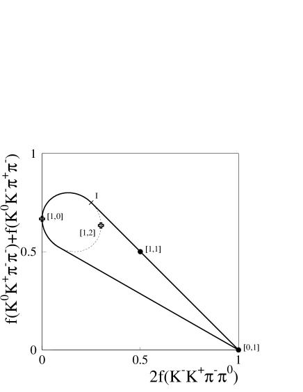
Figure 2: Projection of the allowed domain on the plane $x/y$, $x=\break 2f_{K^{+}K^{-}\pi^{+}\pi^{-}\pi^{-}}$, $y=f_{K^{0}K^{-}\pi^{+}\pi^{-}\pi^{0}}+f_{K^{+}\bar{K}^{0}\pi^{-}\pi^{-}\pi^{0}}$. The classes of amplitudes are labelled by the isospin values and symmetry classes, $[I_{K\bar{K}},(n_{1}n_{2}n_{3})^{I_{3\pi}}]$.

The sub-domains are points for the classes $[0,(300)^{1}]$, $[0,(210)^{1}]$, $[1,(300)^{1}]$ and $[1,(111)^{0}]$. For the interfering classes $[1,(210)^{1}]$ and $[1,(210)^{2}]$, the plane of the two-dimensional sub-domain is determined by the two relations: $\Gamma_{K^{0}K^{-}\pi^{0}\pi^{0}\pi^{0}}=0$ and

$$2(1+{\textstyle 1\over\textstyle\sqrt{3}})\Gamma_{K^{+}K^{-}\pi^{-}\pi^{0}\pi^{0}}+2(1-{\textstyle 1\over\textstyle\sqrt{3}})\Gamma_{K^{+}K^{-}\pi^{+}\pi^{-}\pi^{-}}-\Gamma_{K^{0}K^{-}\pi^{+}\pi^{-}\pi^{0}}-{\textstyle 1\over\textstyle 3}\Gamma_{K^{+}K^{0}\pi^{-}\pi^{-}\pi^{0}}=0.$$

The boundary is given by the saturation of the Schwarzโ€™s inequality $|{\cal I}|=|{\cal I}|_{max}$. The complete, four-dimensional domain is the convex hull of this two-dimensional sub-domain and the four points.

Two-dimensional projections can be constructed by the same method that we used in the previous section. The example shown on Fig. 2 takes $x=2f_{K^{+}K^{-}\pi^{+}\pi^{-}\pi^{-}}$ fraction of decays without neutral hadron and $y=f_{K^{0}K^{-}\pi^{+}\pi^{-}\pi^{0}}+f_{K^{+}\bar{K}^{0}\pi^{-}\pi^{-}\pi^{0}}$ fraction of decays with one $\pi^{0}$ and one $K^{0}$. The complement $1-x-y$ is the fraction of decays with two or three $\pi^{0}$โ€™s. The ellipse bounding the projection of the two-dimensional sub-domain goes through the two points $[1,(210)^{1}]$ and $[1,(210)^{2}]$. It is tangent to the lines $x=0$ and $x+y=1$, since, due to the interference, the contributions of the two classes of amplitudes $[1,(210)^{1}]$ and $[1,(210)^{2}]$ can cancel out in $\Gamma_{K^{+}K^{-}\pi^{+}\pi^{-}\pi^{-}}$ or in $\Gamma_{K^{+}K^{-}\pi^{0}\pi^{0}\pi^{-}}$ and there is no contribution to $\Gamma_{K^{0}K^{-}\pi^{0}\pi^{0}\pi^{0}}$ from $[1,(210)^{1}]$ and $[1,(210)^{2}]$ amplitudes. The boundary of the projected domain is made of two arcs of the curve, four tangents and a segment of the line $\,y=0$. Due to the interference, the ratio of the number of decays with two or three $\pi^{0}$โ€™s over the number of decays without $\pi^{0}$ is only bounded by 0 and 1. The fraction of decays with two or three $\pi^{0}$โ€™s is always lower than 1/2.

To distinguish two $\pi^{0}$ from three $\pi^{0}$ decays, we can use a third coordinate $\,z=f_{K^{0}K^{-}\pi^{0}\pi^{0}\pi^{0}}$. The three-dimensional domain is the cone having for basis the above described contour in the $x/y$ plane and, for vertex, the point $[1,(300)^{1}]$.

5 Summary

We have presented the complete isospin constraints on the $\tau\to K\bar{K}n\pi\nu$ decay modes in the space of charge configurations with some details in the cases $n=2$ and $n=3$.

The geometrical method adopted allows to draw very easily any wanted projection of the multi-dimensional domain and hence obtain the most restrictive inequalities for a given set of measurements.

References

  • [1] F.J. Gilman and S.H. Rhie, Phys. Rev. D 31 (1985) 1066
  • [2] A. Rougรฉ, Z. Phys. C70 (1996) 109
  • [3] A. Pais, Ann. Phys. 9 (1960) 548
  • [4] A. Pais, Ann. Phys. 22 (1963) 274
  • [5] H. Pilkuhn, Nucl. Phys. 22 (1961) 168
  • [6] L. Michel, Nuovo Cim. 22 (1961) 203