Nucleon Instability in SUSY Models

Abstract

A review of the current status of nucleon stability in SUSY unified models is given. The review includes analysis of nucleon stability in the minimal SU(5) supergravity model, and in extensions of the minimal model such as SO(10) models, and models including textures. Implications of the simultaneous constraint of the experimental limit on the proton lifetime and the constraint that dark matter not overclose the universe are also discussed.

1.   Introduction

This review concerns the status of nucleon stability in supersymmetric theories. First, we will give a general discussion of baryon number violation relevant to proton stability in SUSY theories. Next we will discuss in some detail the predictions of nucleon stability in the minimal supergravity model. Finally, we will discuss proton stability in extensions of the minimal model and comment on the issue of proton stability in string models. There are, of course, many sources of baryon number violation in unified theories. First, grand unifed theories have lepto-quark mediated proton decay and in SU(5) the proton decay via lepto-quarks is given by[1]

$$\tau(p\rightarrow e^{+}\pi^{0})\approx(\frac{M_{V}}{3.5\times 10^{14}GeV})^{4}10^{31\pm 1}yr$$ (1)

In SUSY SU(5) models one estimates $M_{V}=1.1\times 10^{16}$ GeV, which gives a p decay lifetime[2] of $1\times 10^{35\pm 1}$. The current limit experimentally is[3]

$$\tau(p\rightarrow e^{+}\pi^{0})>9\times 10^{32}yr,(90\%CL)$$ (2)

and it is expected that Super Kamionkande (Super-K) and Icarus will be able to probe the $e^{+}\pi^{0}$ proton decay mode up to[4] $1\times 10^{34}$y. Thus the $e^{+}\pi^{0}$ mode in SUSY SU(5) may be on the edge of detection if Super-K and Icarus reach their their maximum sensitivity.

In supersymmetric theories there are sources of proton instability arising from terms in the superpotential. The main purpose of this talk is to review the status of proton stability in the presence of these additional sources. The outline of the rest of the paper is as follows: In Sec.2 we discuss B and L violation in supersymmetric theories from the superpotential terms and show that generically even with R parity invariance there is p decay from dimension five operators in SUSY/string unified models. In Sec. 3 we discuss p decay in the minimal SU(5) model. In sec. 4 we discuss p decay in extensions of the minimal model. Conclusions are given in Sec. 5.

2. Sources of P Decay in SUSY/String Models

We turn now to a discussion of the sources B and L violating interactions in the superpotential and their effect on proton stability. It is well known that B and L violating dim 4 operators lead to fast proton decay. Thus, for example, the effective dimension four low energy $SU(3)\times SU(2)\times U(1)$ invariant interaction given by

$$W=\lambda_{u}Qu^{c}H_{2}+\lambda_{d}Qd^{c}H_{1}+\lambda_{e}Le^{c}H_{1}+\mu H_{1}H_{2}$$

$$+(\lambda_{B}^{\prime}u^{c}d^{c}d^{c}+\lambda_{L}^{\prime}Qd^{c}L+\lambda_{L}^{\prime\prime}LLe^{c})$$ (3)

The terms in the bracket lead to fast proton decay and consistency with experiment requires the constraint

$$\lambda_{B}^{\prime}\lambda_{L}^{\prime}<O(10^{-27})$$ (4)

This type of decay is eliminated in the MSSM by the imposition of R parity invariance [where $R=(-1)^{3B+L+2S}$]. It is likely that this discrete R symmetry is remnant of a global continuos R symmetry. In that case there is the danger that the global symmetry may not be preserved by gravitational interactions. For example, worm holes can generate baryon number violating dimension 4 operators and catalize proton decay[5]. A decay of this type is not suppressed by either a large exponential suppression or by a large heavy mass and is thus very rapid and dangerous.

One way to protect against wormhole induced fast proton decay of the type discussed above is to elevate the relevant global symmetries which kill B and L violating dimension 4 operators to gauge symmetries[6, 7]. In this case if the local symmetry breaks down to a discrete symmetry, then the left over discrete symmetry will be sufficient still to protect againt worm hole type induced proton decay. There is, however, the problem that in unified theories undesirable proton decay can arise as a consequence of spontaneous symmetry breaking even if the dangerous dimension 4 operators were forbidden initially. Thus, for example, for SO(10) one can have a interaction of the type $(16)^{4}$ which gives terms of the following type in the superpotential

$$\frac{1}{m_{Pl}}u^{c}d^{c}d^{c}\nu^{c},\frac{1}{m_{Pl}}QLd^{c}\nu^{c}$$ (5)

If there is a spontaneous generation of VEV for the $\nu^{c}$ field, then terms of the type $u^{c}d^{c}d^{c}$ and terms of the type $QLd^{c}$ emerge which once again lead to a rapid proton decay unless $<\nu^{c}>/M_{Pl}$ is O($10^{-13}$). Thus one must make certain that higher dimensional operators in the superpotential do not lead to dangerous p decay after spontaneous symmetry breaking takes place or that spontaneous symmetry breaking does not occur.

Next we discuss p decay from dimension 5 operators (dimension 4 in the superpotential) which contain B and L violating interactions. Using $SU(3)$ $\times$ $SU(2)$ $\times$ $U(1)$ invariance one can write many B and L violating interactions. Examples of such terms in the superpotential involving matter fields are

$$QQQL,~{}~{}u^{c}u^{c}d^{c}e^{c}$$ (6)

One can also have terms which involve the Higgs, e.g.,

$$QQQH_{1},Qu^{c}e^{c}H_{1},etc.$$ (7)

The second set of terms can be eliminated if we impose R parity invariance. However, B and L violating terms of the first type arise quite naturally in SUSY unified models via the exchange of color Higgs triplet fields. In fact we now show that most SUSY/string models will exhibit p instability via the Higgs triplet couplings. The p decay arising from the color Higgs exchange is governed by the interactions[8]

$$\bar{H}_{1}J+\bar{K}H_{1}+\bar{H}_{i}M_{ij}H_{j}$$ (8)

where J and K are quadratic in the matter fields. It is then easily seen that the p decay from dimension five operators is suppressed provided

$$(M^{-1})_{11}=0$$ (9)

Now a condition of this type can be met in one of the following two ways: (i) discrete symmetries, and (ii) non-standard embeddings. However, most SUSY/string models do not normally have discrete symmetries of the desired type which automatically satisfy Eq.(9), and only very specific SUSY/string models (the flipped models[9]) satisfy (ii). Thus in general SUSY/string models do not have a natural suppression of p decay via dimension 5 operators. Thus suppression of p decay here must be forced by making the Higgs triplets heavy.

3.   Proton Decay in Minimal SU(5) SUGRA Model

We begin with a discussion of the comparison of the minimal SU(5) model predictions for the gauge coupling constants at the electro-weak scale with the LEP data. It is well known that the model with the MSSM spectrum extrapolated to high energy gives a reasonably good fit for the coupling constants with experiment[10]. However, a more accurate analysis shows that the theoretical value of $\alpha_{s}$ predicted by SU(5) is about $2\sigma$ higher than experiment[11, 12]. There are a variety of ways in which one can achieve a correction of size $2\sigma$. These include Planck scale corrections, and various other extensions of the minimal SU(5). We discuss here briefly the possibility of Planck scale corrections which are expected to be of size O(M/$M_{Pl}$) where M is size of the GUT scale. It is reasonable to expect that such corrections are present due to the proximity of the GUT scale to the Planck scale. Effects of this size can arise via corrections to the gauge kinetic energy function[12, 13, 14]. For example, for the case of SU(5) one can introduce a field dependence in the the gauge kinetic energy function scaled by the Planck mass so that

$$f_{\alpha\beta}=(\delta_{\alpha\beta}+\frac{c}{2M_{P}}d_{\alpha\beta\gamma}\Sigma^{\gamma})$$ (10)

Here c parametrizes Planck physics and $\Sigma$ is the 24-plet of SU(5). The analysis shows that it is easy to generate a 2$\sigma$ correction to $\alpha_{s}$ with a $c\sim 1$ to achieve full agreement with experiment[12]. It is also possible to understand a 2 $\sigma$ effect on $\alpha_{s}$ from corrections arising from extensions of the minimal SU(5) model such as, for example, in some modified versions of the missing doublet model[15].

Computation of the Higgsino mediated proton decay lifetime in supersymmetric theories involves both GUT physics as well as physics in the low energy region via dressing loop diagrams which convert dimension five operators into dimension six operators which can be used for the computation of proton decay amplitudes[16, 17]. Now the dressings involve 28 separate sparticle masses and many trilinear couplings which mix left and right squark fields. Thus is general no quantitative predictions of proton decay can be made in the MSSM which has a large number of arbitrary parameters in it. In the minimal SUGRA model[18, 19] the number of arbitrary parameters is vastly reduced. Using the constraints of radiative breaking of the electro-weak symmetry one has only four arbitrary parameters and one sign in the SUSY sector of the theory. These can be chosen to be

$$m_{0},m_{\frac{1}{2}},A_{0},tan\beta,sign(\mu)$$ (11)

where $m_{0}$ is the universal scalar mass, $m_{\frac{1}{2}}$, is the universal gaugino mass, $A_{0}$ is the universal trilinear coupling, $tan\beta=<H_{2}>/<H_{1}>$. Here $H_{1}$ gives mass to the down quark and $H_{2}$ gives mass to the up quark, and $\mu$ is the Higgs mixing parameter. Because of the small number of parameters, the minimal supergravity model is very predictive. In turns out that as a consequence of radiative breaking of the electro-weak symmetry, over most of the parameter space of the minimal supergravity model one finds that scaling laws hold and one has[20]

$$m_{\tilde{W}_{1}}\sim\frac{1}{3}m_{\tilde{g}}~{}(\mu<0);m_{\tilde{W}_{1}}\sim\frac{1}{4}m_{\tilde{g}}~{}(\mu>0)$$

$$2m_{\tilde{Z}_{1}}\sim m_{\tilde{W}_{1}}\sim m_{\tilde{Z}_{2}};m_{\tilde{Z}_{3}}\sim m_{\tilde{Z}_{4}}\sim m_{\tilde{W}_{2}}>>m_{\tilde{Z}_{1}}$$

$$m_{H}^{0}\sim m_{A}\sim m_{H^{\pm}}>>m_{h}$$ (12)

In the following we shall use the framework of supergravity to compute proton decay amplitudes. For concreteness we shall use the minimal SU(5) as the GUT group and extensions to the non-minimal case will be discussed in the next section.

The interactions which govern proton decay in minimal SU(5) are given by

$$W_{Y}=-\frac{1}{8}f_{1ij}\epsilon_{uvwxy}H_{1}^{u}M_{i}^{vw}M_{j}^{xy}+f_{2ij}\bar{H}_{2u}\bar{M}_{iv}M_{j}^{uv}$$ (13)

After breakdown of the GUT symmetry and integration over the Higgs triplet field the effective dimension five interaction below the GUT scale which governs p decay is given by[17]

$$\it L^{L}_{5}=\frac{1}{M}\epsilon_{abc}(Pf_{1}^{u}V)_{ij}(f_{2}^{d})_{kl}(\tilde{u}_{Lbi}\tilde{d}_{Lcj}(\bar{e}^{c}_{Lk}(Vu_{L})_{al}-\nu^{c}_{k}d_{Lal})+...)+H.c.$$

$$\it L^{R}_{5}=-\frac{1}{M}\epsilon_{abc}(V^{\dagger}f^{u})_{ij}(PVf^{d})_{kl}(\bar{e}^{c}_{Ri}u_{Raj}\tilde{u}_{Rck}\tilde{d}_{Rbl}+...)+H.c.$$ (14)

where $L^{L}_{5}$ is the LLLL dimension five operator and $L^{R}_{5}$ is the RRRR dimension five operator. The Yukawa couplings can be related to the quark masses at low energy by

$$m_{i}^{u}=f_{i}^{u}(sin2\theta_{W}/e)M_{Z}sin\beta$$

$$m_{i}^{d}=f_{i}^{d}(sin2\theta_{W}/e)M_{Z}sin\beta$$ (15)

and $P_{i}$ are the inter generational phases given by

$$P_{i}=(e^{i\gamma_{i}}),~{}\sum_{i}\gamma_{i}=0;~{}i=1,2,3$$ (16)

There are many possible decay modes of the proton. The most dominant of these are those which involve pseudo-scalar bosons and leptons. These are

$$\bar{\nu}_{i}K^{+},\bar{\nu}_{i}\pi^{+};i=e,\mu,\tau$$

$$e^{+}K^{0},\mu^{+}K^{0},e^{+}\pi^{0},\mu^{+}\pi^{0},e^{+}\eta,\mu^{+}\eta$$ (17)

One can get an estimate of their relative strengths by the quark mass factors and by the CKM factors that appear in their decay amplitudes. These are listed in Table 1. Additionally the decay amplitudes are governed by relative contributions of the third generation vs second generation squark and slepton exchange in the loops. The relative contribution of the third generation vs second generation exchange in the loops is governed by the ratios $y^{tK}$, $y^{t\pi}$,..etc. These are also listed in Table 1.

Table 1: lepton + pseudoscalar decay modes of the proton [17]
SUSY Mode	quark factors	CKM factors	3rd generation enhancement
$\bar{\nu}_{e}K$	$m_{d}m_{c}$	$V_{11}^{\dagger}V_{21}V_{22}$	$(1+y_{1}^{tK})$
$\bar{\nu}_{\mu}K$	$m_{s}m_{c}$	$V_{21}^{\dagger}V_{21}V_{22}$	$(1+y_{2}^{tK})$
$\bar{\nu}_{\tau}K$	$m_{b}m_{c}$	$V_{31}^{\dagger}V_{21}V_{22}$	$(1+y_{3}^{tK})$
$\bar{\nu}_{e}\pi,\bar{\nu}_{e}\eta$	$m_{d}m_{c}$	$V_{11}^{\dagger}V_{21}^{2}$	$(1+y_{1}^{t\pi})$
$\bar{\nu}_{\mu}\pi,\bar{\nu}_{\mu}\eta$	$m_{s}m_{c}$	$V_{21}^{\dagger}V_{21}^{2}$	$(1+y_{2}^{t\pi})$
$\bar{\nu}_{\tau}\pi,\bar{\nu}_{\tau}\eta$	$m_{b}m_{c}$	$V_{31}^{\dagger}V_{21}^{2}$	$(1+y_{3}^{t\pi})$
$eK$	$m_{d}m_{u}$	$V_{11}^{\dagger}V_{12}$	$(1+y_{e}^{tK})$
$\mu K$	$m_{s}m_{u}$		$(1-V_{12}V^{\dagger}_{21}-y_{\mu}^{tK})$
$e\pi,e\eta$	$m_{d}m_{u}$		$(1-V_{11}V^{\dagger}_{11}-y_{e}^{t\pi})$
$\mu\pi,\mu\eta$	$m_{s}m_{u}$	$V_{11}^{\dagger}V_{21}^{\dagger}$	$(1+y_{\mu}^{t\pi})$

Taking all these factors into account one can arrive at the following rough hierarchy of branching ratios.

$$BR(\bar{\nu}K)>BR(\bar{\nu}\pi)>BR(\it lK)>BR(\it l\pi)$$ (18)

The most dominant decay mode of the proton normally is $\bar{\nu}K^{+}$. This pattern can be modified in some situations because of the interference of the contributions from the third generation vs second generation making $\bar{\nu}\pi^{+}$. the most dominant decay mode. However, aside from this special situation which may correspond to fine tuning, the most dominant decay will be $\bar{\nu}K^{+}$. We discuss now the details of this decay mode in minimal supergravity. The $p\rightarrow\bar{\nu}_{i}K^{+}$ decay width for the neutrino type $\nu_{i}$ is given by[17]

$$\Gamma(p\rightarrow\bar{\nu}_{i}K^{+})=(\frac{\beta_{p}}{M_{H_{3}}})^{2}|A|^{2}|B_{i}|C$$ (19)

Here $M_{H_{3}}$ is the Higgs triplet mass and $\beta_{p}$ is the matrix element between the proton and the vacuum state of the 3 quark operator so that

$$\beta_{p}U_{L}^{\gamma}=\epsilon_{abc}\epsilon_{\alpha\beta}<0|d_{aL}^{\alpha}u_{bL}^{\beta}u_{cL}^{\gamma}|p>$$ (20)

where $U^{\gamma}_{L}$ is the proton spinor. The most reliable evaluation of $\beta_{p}$ comes from lattice gauge calculations and is given by[21]

$$\beta_{p}=(5.6\pm 0.5)\times 10^{-3}GeV^{3}$$ (21)

The other factors that appear in Eq.(19) have the following meaning: A contains the quark mass and CKM factors, $B_{i}$ are the functions that describe the dressing loop diagrams, and C contains chiral Lagrangian factors which convert a the Lagrangian involving quark fields to the effective Lagraingian involving mesons and baryons. Individually these functions are given by

$$A=\frac{\alpha_{2}^{2}}{2M_{W}^{2}}m_{s}m_{c}V_{21}^{\dagger}V_{21}A_{L}A_{S}$$ (22)

where $V_{ij}$ are the CKM factors, and $A_{L}$ and $A_{R}$ are the long distance and the short distance renormalization group suppression factors as one evolves the operators from the GUT scale down to the electro-weak scale.$B_{i}$ are given by

$$B_{i}=\frac{1}{sin2\beta}\frac{m_{i}^{d}V_{i1}^{\dagger}}{m_{s}V_{21}^{\dagger}}[P_{2}B_{2i}+\frac{m_{t}V_{31}V_{32}}{m_{c}V_{21}V_{22}}P_{3}B_{3i}]$$ (23)

where the first term in the bracket is the contribution from the second generation and the second term is the contribution from the third generation. The functions $B_{ji}$ are the loop intergrals defined by

$$B_{ji}=F(\tilde{u}_{i},\tilde{d}_{j},\tilde{W})+(\tilde{d}_{j}\rightarrow\tilde{e}_{j})$$ (24)

where

$$F(\tilde{u}_{i},\tilde{d}_{j},\tilde{W})=[Ecos\gamma_{-}sin\gamma_{+}\tilde{f}(\tilde{u}_{i},\tilde{d}_{j},\tilde{W}_{1})+cos\gamma_{+}sin\gamma_{-}\tilde{f}(\tilde{u}_{i},\tilde{d}_{j},\tilde{W}_{1})]$$

$$-\frac{1}{2}\frac{\delta_{i3}m_{i}^{u}sin2\delta_{ui}}{\sqrt{2}M_{W}sin\beta}[Esin\gamma_{-}sin\gamma_{+}\tilde{f}(\tilde{u}_{i1},\tilde{d}_{j},\tilde{W}_{1})-cos\gamma_{-}cos\gamma_{+}\tilde{f}(\tilde{u}_{i1},\tilde{d}_{j},\tilde{W}_{2})$$

$$-(\tilde{u}_{i1}\rightarrow\tilde{u}_{i2})]$$ (25)

and $\tilde{f}$ is given by

$$\tilde{f}(\tilde{u}_{i},\tilde{d}_{j},\tilde{W}_{k})=sin^{2}\delta_{ui}\tilde{f}(\tilde{u}_{i1},\tilde{d}_{j},\tilde{W}_{k})+cos^{2}\delta_{ui}\tilde{f}(\tilde{u}_{i2},\tilde{d}_{j},\tilde{W}_{k})$$ (26)

with

$$f(a,b,c)=\frac{m_{c}}{m_{b}^{2}-m_{c}^{2}}[\frac{m_{b}^{2}}{m_{a}^{2}-m_{b}^{2}}ln(\frac{m_{a}^{2}}{m_{b}^{2}})-(m_{a}\rightarrow m_{c})]$$ (27)

$\gamma_{\pm}=\beta_{+}\pm\beta_{-}$,

$$sin2\beta_{\pm}=\frac{(\mu\pm\tilde{m}_{2})}{[4\nu_{\pm}^{2}+(\mu\pm\tilde{m}_{2})^{2}]^{1/2}}$$ (28)

and

$$\sqrt{2}\nu_{\pm}=M_{W}(sin\beta\pm cos\beta)$$ (29)

$$sin2\delta_{u3}=-\frac{-2(A_{t}+\mu ctn\beta)m_{t}}{m_{\tilde{t}_{1}}^{2}-m_{\tilde{t}_{2}}^{2}}$$ (30)

$$E=1~{},sin2\beta>\mu\tilde{m}_{2}/M_{W}^{2}$$

$$~{}~{}~{}=-1,sin2\beta<\mu\tilde{m}_{2}/M_{W}^{2}$$ (31)

Finally C is given by

$$C=\frac{m_{N}}{32\pi f_{\pi}^{2}}[(1+\frac{m_{N}(D+F)}{m_{B}})(1-\frac{m_{K}^{2}}{m_{N}^{2}})]^{2}$$ (32)

where $f_{\pi},D,F,..$ etc are the chiral Lagrangian factors and have the numerical values: $f_{\pi}=139$ MeV,D=0.76,F=0.48,$m_{N}$=938  MeV,  $m_{K}$=495  MeV, and  $m_{B}$=1154.

The proton can also decay into vector bosons and these modes consist of

$$\bar{\nu}_{i}K^{*},\bar{\nu}_{i}\rho,\bar{\nu}_{i}\omega;i=e,\mu,\tau$$

$$eK^{*},\mu K^{*},e\rho,\mu\rho,e\omega,\mu\omega$$ (33)

A similar analysis can be done for these modes[22].

We discuss now details of the analysis in minimal supergravity unification. In the analysis one looks for the maximum lifetime of the proton as we span the parameter space of the minimal model within the naturalness constraints which we take to be

$$m_{0}\leq 1TeV,m_{\frac{1}{2}}\leq 1Tev,tan\beta\leq 25$$ (34)

In Fig. 1 we display the results of the maximum lifetime for the mode $p\rightarrow\bar{\nu}K^{+}$ as a function of the gluino mass. The analysis indicates that if Super-K and Icarus can reach the maximum sensitivity of $2\times 10^{32}$ y for this mode[4, 23] then most of the parameter space within the naturalness limits indicated will be exhausted. The analysis including the dark matter constraints was also carried out. In this analysis we impose the very conservative constraint that the mass density of the relic neutralinos in the universe not exceed the critical relic density needed to close the universe. The results are also displayed in Fig 1. Here one finds that this constraint limits the maximum gluino mass to lie below 500 GeV[24]. Most of this gluino mass range can be explored at the upgraded Tevatron with an integrated luminosity of about[25, 26] 25$fb^{-1}$.

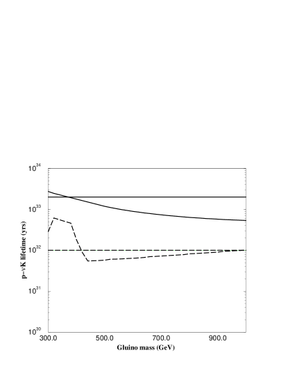
Figure 1: Plot of the maximum $p\rightarrow\bar{\nu}K^{+}$ lifetime under the constraint $m_{0}\leq 1$ TeV in minimal supergravity model. The solid curve is for the case when no relic density constraint is imposed.The dashed curve is with the dark matter constraint $\Omega h^{2}<1$. The dashed horizontal line is the current experimental limit and the solid horizontal line is the limit expected at Super-K and Icarus experiments.

5. Nucleon Stability in Extensions of the Minimal Model

In Sec. 4 we discussed the situation regarding proton decay in the minimal SU(5) supergravity model. We discuss now the situations in some extensions of the minimal model. There are various kinds of extensions of the minimal SU(5) model. These include extension to larger groups, inclusion of textures, flipped models, string models, etc. We will consider here mostly the first two. In SO(10) one has a large tan$\beta$, i.e., tan$\beta\sim 50$ to achieve $b-t-\tau$ unification and compatibity with the observed mass ratios for b, t and $\tau$. However, a large tan$\beta$ tends to destabilize the proton[27]. This can be seen from the fact that the current lower experimental limits for the proton lifetime for this decay mode impose the following constraint on the effective mass scale $M_{PD}\equiv(M^{-1})_{11}$

$$M_{PD}>tan\beta(0.57\times 10^{16})GeV$$ (35)

which for tan$\beta=50$ gives $M_{PD}\sim 2.5\times 10^{17}$ GeV. However, this large scale tends to upset the unification of the gauge coupling constants[27, 28]. The analysis of $\alpha_{s}$ vs $sin^{2}(\theta_{W})$ is plotted in Fig.2 taken from ref.[27]. One finds that for values of $M_{PD}$ of O($10^{17}$) GeV, the disagreement of the theoretical value of $\alpha_{s}$ in minimal SO(10) with experiment is about $6\sigma$[27]. Thus one needs large threshold corrections at the GUT scale to achieve agreement with data[29].

Figure 2: Contour plot of $M_{H_{3}}^{(0)}$ in $sin^{2}(\theta_{W})$ - $\alpha_{3}(M_{Z})$ plane. The dashed line corresponds to the lower bound on $M_{PD}$ in minimal SU(5) of $1.2\times 10^{16}$ GeV. The dot-dashed line corresponds to the lower limit on $M_{PD}$ in minimal SO(10) of $2.7\times 10^{17}$ GeV. Currently, the measurements are $sin^{2}(\theta_{W})=0.2313\pm 0.0003$ and $\alpha_{3}(M_{Z})=0.119\pm 0.0003$ (from ref.[27]).

Next we turn to another type of extension of the minimal SU(5) model and it involves inclusion of textures to generate the correct quark-lepton mass hierarchies[30]. One procedure to generate the textures is to include Planck scale corrections in the superpotential[31, 32], where the Planck scale corrections involve expansions in the ratio $\Sigma/M_{Pl}$, and $\Sigma$ is the adjoint scalar field. After spontaneous breaking of the GUT group $\Sigma$ develops a VeV and one gets a hierarchy in the ratio $M/M_{Pl}$ which allows one to generate the textures in the Higgs doublet sector defined by

$$W_{d}=H_{1}lA^{E}e^{c}+H_{1}d^{c}A^{D}q+H_{2}u^{c}A^{U}q$$ (36)

where $A^{E}$, $A^{D}$ and $A^{U}$ are the textures matrices. Once the textures in the Higgs doublet sector are fixed one can compute the textures in the Higgs triplet sector defined by

$$W_{t}=H_{1}lB^{E}q+H_{2}u^{c}B^{U}e^{c}+\epsilon_{abc}(H_{1}d^{c}_{b}B^{D}u^{c}_{c}+H_{2}^{a}u^{c}_{b}C^{U}d_{c})$$ (37)

where $B^{E}$, $B^{U}$, $B^{D}$, and $C^{U}$ are the triplet textures.

For the case when one adds the most general Planck scale interaction one finds that fixing the textures in the Higgs doublet sector does not uniquely fix the textures in the Higgs triplet sector[32]. One needs a dynamical principle to do so. One possibility suggested is to extend supergravity models to include not only the usual visible and hidden sectors, but also an exotic sector[32]. The exotic sector contains new fields which transform non-trivially under the GUT group and couple to the fields in the hidden sector and the adjoint scalars in the visible sector. After spontaneous supersymmetry breaking the exotic fields develop Planck scale masses because of their couplings with the hidden sector fields and integration over the exotic fields leads to the desired Planck scale corrections. For the choice of a minimal set of exotic fields one finds that the Planck scale corrections are uniquely determined and one finds that correspondingly the textures in the Higgs triplet sector are uniquely determined.

We give now some specifics. The simplest examples of textures are the Georgi-Jarlskog matrices given by

$$A^{E}=\left(\matrix{0&F&0\cr F&-3E&0\cr 0&0&D\cr}\right),A^{D}=\left(\matrix{0&Fe^{i\phi}&0\cr Fe^{-i\phi}&E&0\cr 0&0&D\cr}\right),A^{U}=\left(\matrix{0&C&0\cr C&0&B\cr 0&B&A\cr}\right)$$ (38)

If one uses the most general Planck scale interaction then fixing the texture in the Higgs doublet sector to be the Georgi-Jarlskog does not fix the textures uniquely in the Higgs triplet sector. However, for the case when one uses the exotic sector hypothesis with the minimal set of exotic fields one finds that the textures in the Higgs sector are uniquely determined and are given by[32]

$$B^{E}=\left(\matrix{0&aF&0\cr a^{*}F&{16\over 3}E&0\cr 0&0&{2\over 3}D\cr}\right),B^{D}=\left(\matrix{0&-{8\over 27}F&0\cr{-8\over 27}F&-{4\over 3}E&0\cr 0&0&-{2\over 3}D\cr}\right)$$ (39)

$$B^{U}=\left(\matrix{0&{4\over 9}C&0\cr{4\over 9}C&0&-{2\over 3}B\cr 0&-{2\over 3}B&A\cr}\right)$$ (40)

where a=$(-{19\over 27}+e^{i\phi})$ and $C^{U}=B^{U}$. Estimates including the textures show modest (i.e. O(1)) modifications in the p decay lifetimes. Further, the various p decay branching ratios are affected differentially and thus measurement of the branching ratios will shed light on the textures and on the nature of physics at the GUT scale.

Finally, we discuss briefly proton stability in string models. It is difficult to make general remarks here as there are a huge variety of string models and further the mechanism of supersymmetry breaking in string theory is not fully understood and thus the nature of soft SUSY breaking parameters is not known. However, there are various types of parametrizations that have been used in the literature. One such parametrization is that of no-scale models where one assumes that at the GUT scale one has $m_{0}=0=A_{0}$ and radiative breaking of the electro-weak symmetry is driven by $m_{\frac{1}{2}}$ and the top mass $m_{t}$. In this case it is shown that the minimal SU(5) would lead to a proton decay via dimension five operators which would be in violation of the existing experimental bounds for the $\bar{\nu}K^{+}$ mode[33]. This difficulty is eliminated in the flipped no-scale models[9] where the $\bar{\nu}K^{+}$ mode is highly suppressed. Of course, as mentioned above there is a huge array of string models and each model must be individually examined to test p stability. Thus an analysis of p stability in three generation Calabi-Yau models can be found in ref[34]. Similarly an analysis of p stability in superstring derived standard like models is given in ref. [35].
7.Conclusion

In this review we have given a brief summary of the current status of proton instability in SUSY, SUGRA and string unified models. One of the important conclusions that emerges is that if the Super-K and Icarus experiments can reach the expected sensitivity of $2\times 10^{34}$ y for the $\bar{\nu}K^{+}$ mode, then one can probe a majority of the parameter space of the minimal SUGRA model within the naturalness constraint of $m_{0}\leq 1$ TeV, $m_{\tilde{g}}\leq 1$ TeV, and $tan\beta\leq 20$. If one includes the additional constraint that the neutralino relic density not exceed the critical matter density needed to close the universe then the gluino mass must lie below 500 GeV to satisfy the current lower limit on the $\bar{\nu}K^{+}$ mode. These results will be tested in the near future in p decay experiments as well by experiments at the Tevatron, LEP2 and the LHC.

Acknowledgements:

This research was supported in part by NSF grant numbers PHY-9602074 and PHY-9722090.

References

References

- [1] M.Goldhaber and W.J. Marciano, Comm.Nucl.Part.Phys.16, 23(1986); P.Langacker and N.Polonsky, Phys.Rev.D47,4028(1993).
- [2] W.J. Marciano, talk at SUSY-97, University of Pennsylvania, Philadelphia, May 27-31, 1997.
- [3] Particle Data Group, Phys.Rev. D50,1173(1994).
- [4] Y.Totsuka, Proc. XXIV Conf. on High Energy Physics, Munich, 1988,Eds. R.Kotthaus and J.H. Kuhn (Springer Verlag, Berlin, Heidelberg,1989).
- [5] G. Gilbert, Nucl. Phys. B328, 159 (1989).
- [6] L. Krauss and F. Wilczek, Phys. Rev. Lett. 62, 1221 (1989).
- [7] L. Ibanez and G.G. Ross, Nucl Phys. 368, 4 (1992).
- [8] R. Arnowitt and P. Nath, Phys. Rev. D49, 1479 (1994).
-
[9]
I.Antoniadis, J.Ellis, J.S.Hagelin and D.V.Nanopoulos,
Phys.Lett.B231,65
(1987); ibid, B205, 459(1988). - [10] For a review see, W.de Boer, Prog.Part. Nucl.Phys.33,201(1994).
- [11] J. Bagger, K. Matchev and D. Pierce, Phys. Lett B348, 443 (1995); P.H. Chankowski, Z. Plucienik, and S. Pokorski, Nucl. Phys. B439,23 (1995).
- [12] T. Dasgupta, P. Mamales and P. Nath, Phys. Rev. D52, 5366 (1995); D. Ring, S. Urano and R. Arnowitt, Phys. Rev. D52, 6623 (1995); S. Urano, D. Ring and R. Arnowitt, Phys. Rev. Lett. 76, 3663 (1996); P. Nath, Phys. Rev. Lett. 76, 2218 (1996).
- [13] C.T. Hill, Phys. Lett. B135, 47 (1984); Q. Shafi and C. Wetterich, Phys. Rev. Lett. 52, 875 (1984).
- [14] L.J. Hall and U. Sarid, Phys. Rev. Lett. 70, 2673(1993); P. Langacker and N. Polonsky, Phys. Rev. D47, 4028 (1993).
- [15] A. Dedes and K. Tamvakis, IOA-05-97; J. Hisano, T. Moroi, K. Tobe and T. Yanagida, Phys. Lett. B342, 138 (1995).
- [16] S. Weinberg, Phys. Rev. D26, 287 (1982); N. Sakai and T. Yanagida, Nucl. Phys.B197, 533 (1982); S. Dimopoulos, S. Raby and F. Wilczek, Phys.Lett. 112B, 133 (1982); J. Ellis, D.V. Nanopoulos and S. Rudaz, Nucl. Phys. B202, 43 (1982); B.A. Campbell, J. Ellis and D.V. Nanopoulos, Phys. Lett. 141B, 299 (1984); S. Chadha, G.D. Coughlan, M. Daniel and G.G. Ross, Phys. Lett.149B, 47 (1984).
- [17] R. Arnowitt, A.H. Chamseddine and P. Nath, Phys. Lett. 156B, 215 (1985); P. Nath, R. Arnowitt and A.H. Chamseddine, Phys. Rev. 32D, 2348 (1985); J. Hisano, H. Murayama and T. Yanagida, Nucl. Phys. B402, 46 (1993); R. Arnowitt and P. Nath, Phys. Rev. 49, 1479 (1994).
- [18] A.H. Chamseddine, R. Arnowitt and P. Nath, Phys. Rev. Lett 29. 970 (1982).
- [19] P.Nath,Arnowitt and A.H.Chamseddine , “Applied N=1 Supergravity” (World Scientific, Singapore, 1984); H.P. Nilles, Phys. Rep. 110, 1 (1984); R. Arnowitt and P. Nath, Proc of VII J.A. Swieca Summer School (World Scientific, Singapore 1994).
- [20] R. Arnowitt and P. Nath, Phys. Rev. Lett. 69, 725 (1992); P. Nath and R. Arnowitt, Phys. Lett. B289, 368 (1992).
- [21] M.B.Gavela et al, Nucl.Phys.B312,269(1989).
- [22] T.C.Yuan, Phys.Rev.D33,1894(1986).
- [23] ICARUS Detector Group, Int. Symposium on Neutrino Astrophsyics, Takayama. 1992.
- [24] P. Nath and R. Arnowitt, Proc. of the Workshop ”Future Prospects of Baryon Instability Search in p-Decay and Oscillation Experiments”, Oak Ridge, Tennesse, U.S.A., March 28-30, 1996, ed: S.J. Ball and Y.A. Kamyshkov, ORNL-6910, p. 59.
- [25] T. Kamon, J. Lopez, P. McIntyre and J.J. White, Phys. Rev.D50,5676 (1994); H. Baer, C-H. Chen, C. Kao and X. Tata, Phys. Rev. D52, 1565 (1995); S. Mrenna, G.L. Kane, G.D. Kribbs, and T.D. Wells, Phys. Rev. D53, 1168 (1996).
-
[26]
D. Amidie and R. Brock, ” Report of the tev-2000 Study Group”,
FERMILAB-PUB-96/082. - [27] S. Urano and R. Arnowitt, hep-ph/9611389.
- [28] K.S. Babu and S.M. Barr, Phys. Rev. D51(1995)2463.
- [29] V. Lucas and S. Raby, Phys. Rev. D54 (1996) 2261; ibid. D55 (1997) 6986.
- [30] H. Georgi and C. Jarlskog, Phys. Lett. B86,297 (1979); J. Harvey, P. Ramon and D. Reiss, Phys. Lett. B92,309 (1980); P. Ramond, R.G. Roberts, G.G. Ross, Nucl. Phys. B406, 19 (1993); L. Ibanez and G. G. Ross, Phys. Lett. 332, 100 (1994); K.S. Babu and R. N. Mohapatra, Phys. Lett.74, 2418 (1995); V. Jain and R. Shrock, Phys. Lett. B35, 83 (1995); P. Binetruy and P. Ramond, Phys. Lett. B350, 49 (1995); K. S. Babu and S.M. Barr, hep-ph/9506261; N. Arkani-Hamed, H.-C. Cheng and L.J. Hall, Phys. Rev. D53, 413 (1996); R.D. Peccei and K. Wang, Phys. Rev. D53, 2712 (1996).
- [31] G. Anderson, S. Raby, S. Dimopoulos, L. Hall, and G.D. Starkman, Phys. Rev. D49, 3660 (1994).
- [32] P. Nath, Phys. Lett. B381, 147 (1996); Phys. Rev. Lett. 76, 2218 (1996).
- [33] P. Nath and R. Arnowitt, Phys. Lett. B289, 308 (1992).
- [34] R. Arnowitt and P. Nath. Phys. Rev. Lett. 62, 2225 (1989).
- [35] A.E. Faraggi, Nucl. Phys. B428, 111 (1994).