Determination of $\alpha_{s}$ from Event Shapes and Power Corrections

Abstract

The size of non-perturbative corrections to event shape observables is predicted to fall like a power of the inverse centre of mass energy. These power corrections are investigated for different observables from e⁺e^--annihilation and compared to the theoretical predictions. Using the latest DELPHI high energy data advantages of determining $\alpha_{s}$ from these predictions are discussed and compared to conventional methods.

1 Introduction

The upgrade of LEP to run at energies above the $Z$-peak induced new possibilities in measuring the running of $\alpha_{s}$. Due to asymptotic freedom, non-perturbative effects become less important at higher energies. Different theoretical frameworks suggest that for event shapes the non-perturbative corrections reduce like the inverse power of the centre of mass energy [1, 2]. Theoretical predictions for this decrease can be used in the measurement of $\alpha_{s}$ independent of event by event hadronization models.

2 $\boldmath\alpha_{s}$ from Mean Event Shapes using Power Corrections

The analytical power ansatz for non-perturbative corrections by Dokshitzer and Webber [2, 3] can be used to determine $\alpha_{s}$ from mean event shapes [4, 5, 6]. This ansatz provides an additive term to the perturbative $\cal O$($\alpha_{s}^{2}$) QCD prediction $\left<f_{\mathrm{p}ert}\right>$:

$$\left<f\right>=\frac{1}{\sigma_{\mathrm{t}ot}}\int f\frac{df}{d\sigma}d\sigma=\left<f_{\mathrm{p}ert}\right>+\left<f_{\mathrm{p}ow}\right>$$ (1)

The power correction is given by

$$\left<f_{\mathrm{p}ow}\right>=a_{f}\cdot\frac{\mu_{I}}{E_{\mathrm{c}m}}\Bigg{[}\bar{\alpha}_{0}(\mu_{I})-\alpha_{s}(\mu)$$

$$-\left(\beta_{0}\cdot\ln{\frac{\mu^{2}}{\mu_{I}^{2}}}+\frac{K}{2\pi}+2\beta_{0}\right)\alpha_{s}^{2}(\mu)\Bigg{]}\quad{\rm.}$$ (2)

$\bar{\alpha}_{0}$ is a non-perturbative parameter accounting for the contributions to the event shape below an infrared matching scale $\mu_{I}$, $K=(67/18-\pi^{2}/6)C_{A}-5N_{f}/9$, $\beta_{0}=(33-2N_{f})/12\pi$ and $a_{f}=4C_{f}/\pi$. Beside $\alpha_{s}$ this formulae contains $\bar{\alpha}_{0}$ as the only free parameter. In order to measure $\alpha_{s}$ this parameter has to be known.

To infer $\bar{\alpha}_{0}$ a combined fit of $\alpha_{s}$ and $\bar{\alpha}_{0}$ to a large set of measurements at different energies [4, 5, 7] is performed. For $E_{\mathrm{c}m}\geq M_{Z}$ only DELPHI measurements are included in the fit. Fig. 2 shows the measured mean values of $\left<1-T\right>$ and $\left<M_{h}^{2}/E_{\mathrm{v}is}^{2}\right>$ as a function of the centre of mass energy together with the results of the fit. The resulting values of $\bar{\alpha}_{0}$ are summarized in Tab. 1.

Table 1: $\bar{\alpha}_{0}$ as determined from mean event shapes.

Observable	$\bar{\alpha}_{0}$ $\pm$ stat. $\pm$ scale	$\chi^{2}/\mbox{ndf}$
$\left<1-T\right>$	$0.531\pm 0.012\pm 0.003$	42/23
$\left<M_{h}^{2}/E_{\mathrm{v}is}^{2}\right>$	$0.434\pm 0.010\pm 0.010$	4.0/14

The extracted $\bar{\alpha}_{0}$ values are around 0.5 as expected in [3], but they are incompatible with each other. As the assumed universality is not given to the precision that is accessible from data, $\bar{\alpha}_{0}$ is individually determined for $\left<1-T\right>$ and $\left<M_{h}^{2}/E_{\mathrm{v}is}^{2}\right>$. The scale error is obtained from varying the renormalization scale $f=\mu^{2}/E_{\mathrm{c}m}^{2}$ from 0.25 to 4 and the infrared matching scale from $1\mbox{Ge\kern-0.86108ptV}$ to $2\mbox{Ge\kern-0.86108ptV}$.

After fixing $\bar{\alpha}_{0}$, the $\alpha_{s}$ values corresponding to the high energy data points can be calculated from Eqs. (1–2). $\alpha_{s}$ is calculated for both observables individually and then combined with an unweighted average. Its error is propagated from the data and combined by assuming full correlation. An additional scale error was calculated by varying $f$ and $\mu_{I}$ in the ranges discussed. The results are summarized in Tab. 2 and plotted as function of $E_{\mathrm{c}m}$ (open dots) together with the QCD expectation in Fig. 2a.

Table 2: $\alpha_{s}$ as obtained from means with the Eqs. (1–2) by averaging the $\left<1-T\right>$ and $\left<M_{h}^{2}/E_{\mathrm{v}is}^{2}\right>$ results.

$E_{\mathrm{c}m}$	$\alpha_{s}(E_{\mathrm{c}m})$ $\pm$	stat. $\pm$	sys. $\pm$	scale
133GeV	0.1162 $\pm$	0.0070 $\pm$	0.0009 $\pm$	0.0047
161GeV	0.1047 $\pm$	0.0069 $\pm$	0.0034 $\pm$	0.0043
172GeV	0.1052 $\pm$	0.0082 $\pm$	0.0037 $\pm$	0.0041

3 $\boldmath\alpha_{s}$ from Event Shapes Distributions

From event shape distributions $\alpha_{s}$ is determined by fitting an $\alpha_{s}$ dependent QCD prediction ($\cal O$($\alpha_{s}^{2}$), pure NLLA or combined $\cal O$($\alpha_{s}^{2}$)+NLLA [8, 9, 10]) folded with a hadronization or a power correction to the data. The fitranges used for the different QCD predictions are shown in Fig. 1. The ranges for pure NLLA and $\cal O$($\alpha_{s}^{2}$) fits are chosen to be distinct, so that the results are statistically uncorrelated.

Figure 1: Fit ranges chosen for fitting $\alpha_{s}$ from different QCD predictions of $1-T$ and $M_{h}^{2}/E_{\mathrm{v}is}^{2}$ distributions.

3.1 Using Hadronization Models

As an example of a Monte Carlo based model in this section the hadronization correction is calculated using the JETSET PS model (Version 7.4 tuned to DELPHI data [11]). The QCD prediction is multiplied in each bin by the correction factor (the model prediction of the ratio of hadron over parton level in that bin).

For $\cal O$($\alpha_{s}^{2}$)-fits the renormalization scale $\mu$ was fitted to the LEP1 data [11] for both observables individually and then fixed for the fits to the high energy distributions. This takes advantage of optimized scales. In contrast for NLLA and combined fits $\mu$ was set equal to $E_{\mathrm{c}m}$, so that these results can be compared to other experiments.

The systematic errors were obtained by fitting several $1-T$ and $M_{h}^{2}/E_{\mathrm{v}is}^{2}$ distributions evaluated by applying different cuts. The mean deviation from the central value is used as systematic error. Scale errors were taken from previous DELPHI publications [12, 13].

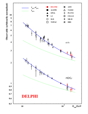
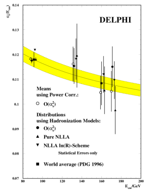
a) b) c)

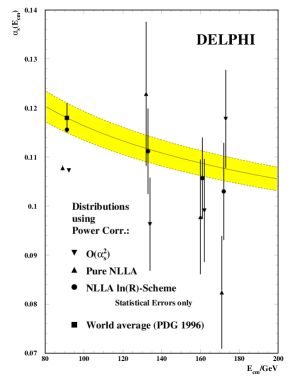
Figure 2: a) Measured mean values of $\left<1-T\right>$ and $\left<M_{h}^{2}/E_{\mathrm{v}is}^{2}\right>$ as a function of the centre of mass energy. The solid lines present the results of the fits with Eqs. (1–2), the dashed lines show the perturbative part.
b) Energy dependence of $\alpha_{s}$. The errors shown are statistical only. The band shows the QCD expectation of extrapolating the world average to other energies.
c) $\alpha_{s}$ determined using Dokshitzer and Webber power corrections with $1-T$ distribution.

The $\alpha_{s}$ values evaluated from the distributions are given in Tab. 3 and shown as a function of $E_{\mathrm{c}m}$ in Fig. 2b. The results agree well with those measured from the event shape means.

3.2 Using Power Corrections

Dokshitzer and Webber recently extended their model of power corrections to event shape distributions [14]. For distributions the power corrections are applied by shifting the complete prediction:

$$F(f)=\frac{1}{\sigma_{\mathrm{t}ot}}\frac{d\sigma}{df}=F_{\mathrm{p}ert}(f-\delta f)$$ (3)

where the size of the shift is given by the size of the power correction to the corresponding mean ($\delta f=\left<f_{\mathrm{p}ow}\right>$). The perturbative prediction $F_{\mathrm{p}ert}$ can now be any of the available QCD predictions: $\cal O$($\alpha_{s}^{2}$), NLLA or any combined scheme.

To measure $\alpha_{s}$ at a single energy, again one first has to determine $\bar{\alpha}_{0}$. This is done in a combined fit of $\bar{\alpha}_{0}$ and $\alpha_{s}$ to measurements [4, 5, 7] at many different energies. See Fig. 3a, c and Tab. 4. For $M_{h}^{2}/E_{\mathrm{v}is}^{2}$ some of the lowest energies were removed from the fit, because the shifted QCD prediction was no longer defined at the lower end of the fit range.

To compare the quality of these fits to a hadronization model based description, a simultaneous fit of $\alpha_{s}$ to these data using the JETSET PS based hadronization correction is done. The results are plotted in Fig. 3b, d and summarized in Tab. 4.

Figure 3: $\cal O$($\alpha_{s}^{2}$) fit of $\alpha_{s}$ (and $\bar{\alpha}_{0}$) to $1-T$ and $M_{h}^{2}/E_{\mathrm{v}is}^{2}$ distributions measured at different energies. In plot a,c the power ansatz Eq. 3, in b,d JETSET PS based correction is used to include non-perturbative contributions. The distributions including dotted lines were not included in the fit.

Using these $\bar{\alpha}_{0}$ results to determine $\alpha_{s}$ from individual high energy $1-T$ distributions lead to systematic deviations from the QCD expectation (See Fig. 2c). The deviation is different for NLLA and $\cal O$($\alpha_{s}^{2}$) (which use different fit ranges) and opposite in sign.

To investigate this problem, the Dokshitzer and Webber power correction term was replaced by a simple ansatz:

$$\delta f=\frac{C_{1}}{E_{\mathrm{c}m}}+\frac{C_{2}}{E^{2}_{\mathrm{c}m}}$$ (4)

A combined fit of $C_{1}$, $C_{2}$ to the complete set of distributions probes the need of the quadratic power correction term. $\alpha_{s}$ was fixed to 0.120 here. It is found, that for the fit ranges used in $\cal O$($\alpha_{s}^{2}$) and NLLA fits of Thrust the correction arising from the quadratic power term is not negligable (See Tab. 5). The small result of $C_{2}$ for the combined result thus may be accidental.

Table 3: $\alpha_{s}$ as obtained from distributions using JETSET.

133GeV	$\alpha_{s}(E_{\mathrm{c}m})$ $\pm$	exp.$\hfil\pm$		scale
$\cal O$($\alpha_{s}^{2}$)	0.1154 $\pm$	0.0072$\hfil\pm$		0.006
NLLA	0.1196 $\pm$	0.0129$\hfil\pm$		0.005
Combined	0.1182 $\pm$	0.0083$\hfil\pm$		0.006
161GeV	$\alpha_{s}(E_{\mathrm{c}m})$ $\pm$	stat. $\pm$	sys. $\pm$	scale
$\cal O$($\alpha_{s}^{2}$)	0.1084 $\pm$	0.0088 $\pm$	0.0049 $\pm$	0.006
NLLA	0.1056 $\pm$	0.0096 $\pm$	0.0043 $\pm$	0.005
Combined	0.1120 $\pm$	0.0074 $\pm$	0.0032 $\pm$	0.006
172GeV	$\alpha_{s}(E_{\mathrm{c}m})$ $\pm$	stat. $\pm$	sys. $\pm$	scale
$\cal O$($\alpha_{s}^{2}$)	0.1151 $\pm$	0.0082 $\pm$	0.0058 $\pm$	0.005
NLLA	0.0976 $\pm$	0.0097 $\pm$	0.0046 $\pm$	0.005
Combined	0.1097 $\pm$	0.0076 $\pm$	0.0029 $\pm$	0.005

Table 4: $\bar{\alpha}_{0}$ as determined from event shape distributions. The error is the statistical error from the fit.

$1-T$	$\bar{\alpha}_{0}$	$\chi^{2}/\mbox{ndf}$
$\cal O$($\alpha_{s}^{2}$)	$0.550\pm 0.012$	120/107
NLLA	$0.475\pm 0.006$	81/26
Combined	$0.491\pm 0.005$	377/137
$M_{h}^{2}/E_{\mathrm{v}is}^{2}$	$\bar{\alpha}_{0}$	$\chi^{2}/\mbox{ndf}$
$\cal O$($\alpha_{s}^{2}$)	$0.698\pm 0.014$	83/49
NLLA	$0.480\pm 0.012$	3.2/7
Combined	$0.554\pm 0.005$	285/53

Table 5: Results of fitting the simple power ansatz to event shape distributions. $\alpha_{s}$=0.120.

$1-T$	$C_{1}[\mbox{Ge\kern-0.86108ptV}]$	$C_{2}[\mbox{Ge\kern-0.86108ptV}^{2}]$
$\cal O$($\alpha_{s}^{2}$)	$1.23\pm 0.09$	$-10.4~{}\pm 1.3$
NLLA	$0.27\pm 0.02$	$+10.0~{}\pm 0.6$
Combined	$0.73\pm 0.02$	$-~{}0.48\pm 0.61$
$M_{h}^{2}/E_{vis}^{2}$	$C_{1}[\mbox{Ge\kern-0.86108ptV}]$	$C_{2}[\mbox{Ge\kern-0.86108ptV}^{2}]$
$\cal O$($\alpha_{s}^{2}$)	$0.27\pm 0.09$	$+14.8~{}\pm 6.9$
NLLA	not converging
Combined	$0.70\pm 0.02$	$-~{}4.5~{}\pm 6.9$

4 Summary/Conclusions

Several methods of determining $\alpha_{s}$ at high energies from event shapes were discussed.

The results from means using power corrections are compatible with those from distributions using standard hadronization corrections. Results from power corrections yield smaller scale errors.

Power corrections to event shape distributions are more tricky.

References

- [1] V. I. Zakharov. In these proceedings.
- [2] Y. L. Dokshitzer and B. R. Webber. Phys. Lett. B352(1995) 451.
- [3] B. R. Webber. Talk given at workshop on DIS and QCD in Paris, hep-ph/9510283, 1995.
- [4] DELPHI Coll., P. Abreu et al. Z. Phys. C573(1997) 229.
- [5] J. Drees, A. Grefrath, K. Hamacher, O. Passon, and D. Wicke. DELPHI 97-92 CONF 77, contrib. to EPS HEPC in Jerusalem, 1997.
- [6] O. Biebel. In these proceedings.
-
[7]
ALEPH Coll., Phys. Lett. B284 (1992) 163.
ALEPH Coll., Z. Phys. C55 (1992) 209.
AMY Coll., Phys. Rev. Lett. 62 (1989) 1713.
AMY Coll., Phys. Rev. D41 (1990) 2675.
CELLO Coll., Z. Phys. C44 (1989) 63.
HRS Coll., Phys. Rev. D31 (1985) 1.
JADE Coll., Z. Phys. C25 (1984) 231.
JADE Coll., Z. Phys. C33 (1986) 23.
L3 Coll., Z. Phys. C55 (1992) 39.
Mark II Coll., Phys. Rev. D37 (1988) 1.
Mark II Coll., Z. Phys. C43 (1989) 325.
MARK J Coll., Phys. Rev. Lett. 43 (1979).
OPAL Coll., Z. Phys. C59 (1993) 1.
PLUTO Coll., Z. Phys. C12 (1982) 297.
SLD Coll., Phys. Rev. D51 (1995) 962.
TASSO Coll., Phys. Lett. B214 (1988) 293.
TASSO Coll., Z. Phys. C45 (1989) 11.
TASSO Coll., Z. Phys. C47 (1990) 187.
TOPAZ Coll., Phys. Lett. B227 (1989) 495.
TOPAZ Coll., Phys. Lett. B278 (1992) 506.
TOPAZ Coll., Phys. Lett. B313 (1993) 475. - [8] R. K. Ellis, D. A. Ross, and A. E. Terrano. Nucl. Phys B178(1981) 412.
- [9] S. Catani, G. Turnock, B. R. Webber, and L. Trentadue. Phys. Lett. B263(1991) 491.
- [10] S. Catani, G. Turnock, and B. R. Webber. Phys. Lett. B272(1991) 368.
- [11] DELPHI Coll., P. Abreu et al. Z. Phys. C73(1996) 11.
- [12] DELPHI Coll., P. Abreu et al. Z. Phys. C54(1992) 21.
- [13] DELPHI Coll., P. Abreu et al. Z. Phys. C59(1993) 21.
- [14] Y. L. Dokshitzer and B. R. Webber. Cavendish-HEP-97/2, hep-ph/9704298, 1997.