Partonometry in W + jet production

Abstract

QCD predicts soft radiation patterns that are particularly simple for $W+\mbox{jet}$ production. We demonstrate how these patterns can be used to distinguish between the parton-level subprocesses probabilistically on an event-by-event basis. As a test of our method we demonstrate correlations between the soft radiation and the radiation inside the outgoing jet.

1 Introduction

Hard scattering in QCD is accompanied by soft radiation of gluons caused by the drastic accelerations of color charge. The resulting antenna patterns are predicted to be particularly simple for $2\to 2$ hard scattering processes in which one of the final particles is colorless [1, 2]. The possibility of using the radiation pattern to identify the underlying parton structure of observed events has been called “partonometry” [1]. In this paper, we address the question of how partonometry can be carried out in practice, and how it can be used to make further studies of QCD.

As a specific example that is accessible to experiment, we study the process $\bar{p}p\to W^{\pm}+{\rm jet}$ at the Fermilab Tevatron energy $\sqrt{s}=1.8\,{\rm TeV}$. The predicted cross section for $p_{\perp}^{\,\rm jet}>30\,{\rm GeV/c}$ with $W\to e\nu$ or $\mu\nu$ is $\approx 180\,{\rm pb}$, which is large enough for an ample number of events to be collected in the CDF and D0 experiments at the Fermilab Tevatron. Similar physics can also be studied in $Z^{0}$ or direct photon + jet production.

At lowest order in QCD, $W+{\rm jet}$ production comes from three incoherent partonic subprocesses:

$$gq\to Wq$$ (1)

$$qg\to Wq$$ (2)

$$q\bar{q}\to Wg$$ (3)

The first two of these are “Compton” subprocesses that are distinguished from each other by the direction of their initial gluon, which is in the $+z$ direction for (1) and $-z$ for (2). The third “annihilation” subprocess has a slightly larger cross section than the sum of the Compton subprocesses, because of the dominance of quarks over gluons in the parton distributions at the moderate values of $x$ involved here.

“Partonometry” in this instance is the ability to recognize which of the three hard subprocesses (1)–(3) was responsible for a given $W+{\rm jet}$ event. In section 2 we will see that the subprocesses have very distinct radiation patterns. These patterns are quite striking, but unfortunately the ability to distinguish them is hampered by large fluctuations of the radiation around these average distributions. To model the fluctuations, as well as the underlying background event and hadronization effects, we use the Monte Carlo program HERWIG [3], which has the correct correlations included to produce the radiation patterns that we seek. In section 3 we define some event variables that are useful for distinguishing the underlying subprocesses. In section 4 we describe the Monte Carlo simulation that we use and show that it reproduces the radiation patterns that we expect, even after the underlying event and hadronization have been included. Our main results are in section 5, where we identify an observable of the soft radiation which can be used to discriminate between the parton-level subprocesses, and we show how this observable can be tested by experiment. Finally, in section 6 we give our conclusions.

2 Radiation Patterns

In the large $N_{c}$ limit, soft gluon radiation from the three basic subprocesses is proportional to [1, 2]

$$\rho_{1} = 1+\frac{\frac{1}{2}\,e^{+\Delta\eta}}{\cosh{\Delta\eta}-\cos{\Delta\phi}}$$ (4)

$$\rho_{2} = 1+\frac{\frac{1}{2}\,e^{-\Delta\eta}}{\cosh{\Delta\eta}-\cos{\Delta\phi}}$$ (5)

$$\rho_{3} = \frac{\cosh{\Delta\eta}}{\cosh{\Delta\eta}-\cos{\Delta\phi}}$$ (6)

for processes (1), (2), and (3), respectively. The “Lego” variables here are defined relative to the jet location:

$$\Delta\eta\equiv\eta-\eta_{\rm jet}$$ (7)

and

$$\Delta\phi\equiv\phi-\phi_{\rm jet},$$ (8)

with $\eta=-\ln\tan\theta/2$ the pseudorapidity and $\phi$ the azimuthal angle. The soft gluon radiation patterns are displayed in cylindrical-coordinate plots in Fig. 1. Here $\Delta\eta$ is along the cylindrical axis, $\Delta\phi$ is the azimuthal angle, and the intensity of the radiation is proportional to the distance from the cylindrical axis. Note that these radiation patterns only depend on the coordinates relative to the jet and are completely independent of the direction of the $W$ boson.

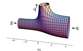
(a)	(b)

Figure 1: Radiation densities (a) $\rho_{1}$ and (c) $\rho_{3}$. $\rho_{2}$ can be obtained from $\rho_{1}$ by the replacement $\Delta\eta\to-\Delta\eta$.

There are three important gross features of the radiation patterns. A first obvious feature is that the radiation patterns are singular in the direction collinear to the outgoing jet. This is exhibited by the fact that the surfaces in Fig. 1 blow up to infinity as $\Delta\eta\to 0$, $\Delta\phi\to 0$. In addition, the radiation from a gluon jet is stronger than radiation from $q$ or $\bar{q}$ as expected: $\rho_{1}=\rho_{2}=\frac{1}{2}\rho_{3}\to 1/[(\Delta\eta)^{2}+(\Delta\phi)^{2}]$ for small $\Delta\eta\mbox{, }\Delta\phi$.

The second general feature is that radiation from the Compton subprocesses is enhanced in the direction of their initial gluon:

$$\left.\begin{array}[]{l}\rho_{1}\to 1\\ \rho_{2}\to 2\\ \rho_{3}\to 1\end{array}\right\}\;\mbox{for}\;\Delta\eta\gg 1\;,\quad\left.\begin{array}[]{l}\rho_{1}\to 2\\ \rho_{2}\to 1\\ \rho_{3}\to 1\end{array}\right\}\;\mbox{for}\;\Delta\eta\ll 1\;.$$ (15)

This enhancement extends arbitrarily far away from the jet in the $(\eta,\phi)$ plane. The large area over which the radiation pattern can be integrated offers the prospect of observing it in a majority of events, even though the observed radiation in any small region of $(\eta,\phi)$ is subject to large fluctuations and is partially masked by the “background event”. Note that we use the variables $\Delta\eta$ and $\Delta\phi$ rather than $\Delta R$ and $\beta$ of Ref. [1] because we have found regions distant from the jet to be important. The relations between these variables are $\Delta\eta=\Delta R\,\cos\beta$ and $\Delta\phi=\Delta R\,\sin\beta$.

The third important gross feature of the radiation pattern is the suppression of radiation from the annihilation subprocess (3) at small $\Delta\eta$ on the side opposite to the jet in azimuthal angle. The extreme of this is

$$\left.\begin{array}[]{l}\rho_{1}\to 1.25\\ \rho_{2}\to 1.25\\ \rho_{3}\to 0.5\end{array}\right\}\;\mbox{for}\;\Delta\eta=0,\Delta\phi=180^{\circ}\;.$$ (19)

These features of the radiation patterns can be seen more quantitatively in Fig. 2, which shows the $\Delta\eta$ distributions averaged over strips $0<|\Delta\phi|<60^{\circ}$ and $120^{\circ}<|\Delta\phi|<180^{\circ}$. Although we use the large $N_{c}$ limit throughout, we note that the $1/N_{c}^{2}$ corrections are small and actually enhance the effects that we are seeking.

(a)	(b)

Figure 2: (a) Soft gluon radiation function averaged over strip $0<|\Delta\phi|<60^{\circ}$. Dashed curve = subprocess (1), Dotted curve = subprocess (2), Solid curve = subprocess (3). (b) Same, but for $120^{\circ}<|\Delta\phi|<180^{\circ}$

3 Event Variables

Before we look for soft radiation patterns in the data, we define some convenient observable quantities in order to highlight the features discussed above. We divide the region outside the jet into forward (F), backward (B) and side (S) regions as in Fig. 3.

Figure 3: Definition of regions F, B and S.

We then define the following scalar sums

$$F=\sum_{+1.25\,<\,\Delta\eta<\,+3.75}|p_{\perp}|\;,$$ (20)

$$B=\sum_{-3.75\,<\,\Delta\eta\,<\,-1.25}|p_{\perp}|\;,$$ (21)

and

$$S=\sum_{|\Delta\eta|<1.25,\;|\Delta\phi|>\pi/2}|p_{\perp}|\;.$$ (22)

With these definitions, we would expect on average that subprocess (1) ($gq\rightarrow Wq$) would have an enhancement in F, subprocess (2) ($qg\rightarrow Wq$) would have an enhancement in B, and subprocess (3) ($q\bar{q}\rightarrow Wg$) would have a deficit in S. We have investigated a number of observable quantities that use this information to distinguish between the underlying subprocesses. The details are given in the appendix. In the main part of the text we will focus on the quantity $|F-B|+S$. It is designed to be sensitive to the differences between events with a final-state quark (1 and 2) and events with a final-state gluon (3). This is because quark-jet events tend to have large forward-backward differences and relatively large radiation in the side region, as we saw in the previous section. Gluon-jet events, on the other hand, tend to have equal forward and backward radiation, in addition to suppression in the side region.

To test this observable, it will be helpful to have another quantity sensitive to the differences between the various subprocesses that does not depend on the properties of the soft radiation. Various ways to measure the radiation inside a jet cone have been invented in order to discriminate between quark jets and gluon jets. They have been validated both by using Monte Carlo simulation [4, 5] and experiment [6]. One suitable variable [5] can be defined by dividing the jet cone of radius $R=0.7$ in $(\eta,\phi)$ into $0.1\times 0.1$ cells, as is typical of calorimetric detectors. The jet $p_{\perp}$ can be defined as the total $p_{\perp}$ detected in all cells in the cone. By sorting these cells in order of their $|p_{\perp}|$, we define the variable

$$X=\mbox{the minimum number of cells needed to include all but $\sqrt{|p_{\perp}|^{\rm tot}}$ of the total $|p_{\perp}|^{\rm tot}$},$$ (23)

where $p_{\perp}$ is given in units of GeV/c. This definition makes the $X$ distribution roughly independent of jet $p_{\perp}$. $X$ can be defined to include a fractional part given by linear or logarithmic interpolation.

4 Simulation

The distinctive radiation patterns of Fig. 2 are predicted by the soft gluon approximation. However, on an event-by-event basis there will be large fluctuations around these average distributions. We must also ask to what extent these patterns survive finite-energy effects and the non-perturbative effects of hadronization, whereby colored partons combine to form physical hadrons. Many of those hadrons are resonances that undergo strong decay before reaching the detector, further broadening structures in the $(\eta,\phi)$ plane. The notion of local parton-hadron duality (LPHD) [7], which is supported by experiment [8], suggests however that the patterns should survive reasonably well.

For quantitative predictions, we simulate $\bar{p}p\to W^{\pm}+{\rm jet}$ using the HERWIG 5.8 [3] Monte Carlo event generator, which contains the color coherence effects we seek and embodies LPHD in its cluster formation and decay model. We make a rather tight cut on the jet transverse momentum ($30<p_{\perp}^{\,\rm jet}<40$ GeV/c) in order to simplify the study. We will also generally make a cut $|\eta_{\rm jet}|<0.5$ on the jet rapidity. These cuts are not essential, and it will be desirable to loosen them for actual data analysis to improve the statistics. In the experiment, the cut on minimum $p_{\perp}^{\,\rm jet}$ should be replaced by a cut on $p_{\perp}^{\,\rm W}$ to avoid biases that depend on jet structure. The effects we seek are somewhat cleaner at higher $p_{\perp}^{\,\rm jet}$, but the cross section falls rather rapidly at large $p_{\perp}^{\,\rm jet}$.

Results from the simulation are shown in Fig. 4 for the same two strips in $\Delta\phi$ as in Fig. 2. The quantity plotted is $\langle p_{\perp}\rangle$ in GeV/c per unit $\Delta\eta\;\Delta\phi$ at $|\eta_{\rm jet}|<0.5\,$. A suppression at large $\eta$ is apparent, so that the “plateau” is not flat. But otherwise, the soft gluon pattern survives very well. In particular the roughly $2:1$ enhancement of subprocesses (1) and (2) in the directions of their incoming gluon at large $\Delta\eta$, and the suppression of subprocess (3) at $\{\eta\approx\eta_{\rm jet},\Delta\phi\approx 180^{\circ}\}$ remain. In generating Fig. 4, the HERWIG option of a contribution from a minimum-bias–like “background event” was turned off. The result of turning it on is shown in Fig. 5. The background event adds extra radiation to each subprocess, so that the differences are largely preserved, while the ratios are substantially diluted.

(a)	(b)

Figure 4: (a) Average $p_{\perp}$ per unit area in $(\eta,\phi)$ for simulated events with $|\eta_{\rm jet}|<0.5$, in the region $0<|\Delta\phi|<60^{\circ}$ (cf. Fig. 2), “background event” off. (b) Same, but for $120^{\circ}<|\Delta\phi|<180^{\circ}$.

(a)	(b)

Figure 5: (a) Average $p_{\perp}$ per unit area in $(\eta,\phi)$ for simulated events with $|\eta_{\rm jet}|<0.5$, in the region $0<|\Delta\phi|<60^{\circ}$ (cf. Fig. 2), “background event” on. (b) Same, but for $120^{\circ}<|\Delta\phi|<180^{\circ}$.

5 Observing the radiation patterns

Each of the partonic subprocesses (1)–(3) is predicted to have its distinctive radiation pattern, as we have seen. Unfortunately, these radiation patterns cannot be observed directly, because for real events — unlike the simulated ones — one does not know which of the three subprocesses is responsible for any given event. To establish this physics with a testable prediction, we must study a global correlation that is based on the fact that any particular event is caused by a single one of the three production subprocesses. Therefore, a typical event should have either enhanced radiation at $\eta\gg\eta_{\rm jet}$; or enhanced radiation at $\eta\ll\eta_{\rm jet}$; or reduced radiation at $\eta\approx\eta_{\rm jet}$, $\Delta\phi\approx 180^{\circ}$. Looking for these characteristics of the radiation in an event-by-event basis is also what is needed to achieve the promise of “partonometry” [1]. Of course, in practice the underlying subprocess can only be determined with some probability, due to fluctuations in the soft radiation patterns.

There are three necessary steps to partonometry. First, we must identify an observable function of the soft radiation that discriminates between partonic subprocesses. Second, we need to be able to test the prediction experimentally. Finally, we need a quantitative measure of the discrimination efficiency of our observable. The second step requires comparison with another event observable that does not depend on the properties of the soft radiation in the event. An observable based on information inside the jet cone is the natural choice.

In what follows we give a concrete example of partonometry using the soft radiation observable $|F-B|+S$. We also use the jet observable $X$ as a cross check of this discriminator. These may or may not prove to be the best variables when detector effects are included. Nonetheless, the procedure should be applicable to a wide variety of observable quantities.

The predictions from HERWIG for $|F-B|+S$ are shown in Fig. 6.

Figure 6: Probability distribution for $|F-B|+S$. Solid curve: quark jets (from subprocess (3)); dotted curve: gluon jets (from subprocesses (1) and (2)).

The differences between the curves satisfy our first criterion above. The predictions from HERWIG for the jet variable $X$ are shown in Fig. 7.

Figure 7: Probability distribution for $X$ defined as the minimum number of cells in the jet cone $R<0.7$ required to contain all but $\sqrt{|p_{\perp}|^{\rm tot}}$ of the total jet $|p_{\perp}|^{\rm tot}$ in the cone, where $p_{\perp}^{\rm tot}$ is given in GeV/c. Solid curve: quark jets (from subprocess (3)); dotted curve: gluon jets (from subprocesses (1) and (2)).

There is a clear difference between the quark jets (subprocess (3)) and the gluon jets (subprocesses (1) and (2)), with the latter tending toward larger values of $X$, i.e., gluon jets are fatter. The correlations between Figs. 6 and 7 provide the qualitative and quantitative tests for our soft radiation predictions.

To observe the correlation, we divide the data sample into bins of $|F-B|+S$ and then calculate the mean value of $X$ in each bin. The result is shown in Fig. 8.

Figure 8: Mean value of $X$ as a function of $|F-B|+S$.

For a pure sample of gluon jets or quark jets, the value of $\langle X\rangle$ increases mildly with $|F-B|+S$, indicating that $\langle X\rangle$ increases with the amount of soft radiation, as one would expect. However, we predict that the combined data will show a decrease in $\langle X\rangle$ with increasing $|F-B|+S$. This is an unambiguous qualitative test of the soft radiation patterns. The decrease comes about because as $|F-B|+S$ increases, the likelihood that the outgoing jet is a quark increases, reducing the value of $\langle X\rangle$. This is shown in Fig. 9, where we plot the fraction of outgoing gluon jets as a function of $|F-B|+S$, as calculated using HERWIG. The gluon or quark jet fraction can be made as high as 80% by focusing on events with very large or small values of $|F-B|+S$, albeit at the expense of statistics.

Figure 9: Fraction of jets which are gluon jets, $g$, as a function of $|F-B|+S$.

Even stronger discrimination between the processes can be achieved by using both variables $|F-B|+S$ and $X$ in tandem.

6 Conclusions

Soft radiation patterns in $W+\mbox{jet}$ production provide a novel insight into the structure of QCD. In this paper we have identified the most important structures in the radiation patterns, and we have defined an observable, $|F-B|+S$, that can be used to distinguish the three partonic subprocesses (1)–(3). We have also shown how this observable can be cross-checked against a second observable, $\langle X\rangle$, which relies only on information from inside the jet cone. The prediction, shown by the solid curve in Fig. 8, is a striking one: we predict a negative correlation between the amount of radiation inside the jet cone and the amount of radiation outside it. This arises solely because more radiation outside the cone is associated with a higher probability of the jet being a quark jet, as shown in Fig. 9. The negative correlation is otherwise opposite to the naive expectation that the radiation outside the cone should rise with the radiation inside – as is confirmed for quark jets alone or gluon jets alone in Fig. 8. The ability to discriminate between the underlying soft radiation patterns is potentially useful as a tool for identifying and studying parton-level subprocesses. One could imagine using this information both as a means to separate the gluon from the quark parton distribution functions in the initial state and as a method to study the differences between quark and gluon jets in the final state.

We emphasize again that the procedure we have outlined for utilizing and testing the soft-radiation effects could be followed for a variety of soft-radiation and jet observables. Further work may be needed in particular to optimize the suggested observables to suit detector limitations. In addition, the details presented here rely on the use of HERWIG for producing the hadronization effects and the background event. Information on jet properties taken directly from experiment [6] may be used to lessen this dependence on the Monte Carlo simulation. The important point is that the soft radiation effects should remain and can be discerned. Observing these patterns is both interesting in its own right and as a novel probe of the underlying partonic structure of QCD.

Appendix

In the text we have used the quantity $|F-B|+S$ to discriminate between the soft radiation patterns from the different event types. Many other possibilities are available. We give some of the alternatives here.

One logical quantity to investigate is the asymmetry

$$A\equiv\frac{F-B}{F+B}.$$ (24)

In the limit where the forward and backward regions extend to infinity, Eqs. (4–6) predict the averages $\langle A\rangle=+1/3,~{}-1/3\mbox{ and }0$ for subprocesses 1, 2, and 3, respectively. This prediction does not include such real-world effects as hadronization and the underlying event, which tends to increase both $F$ and $B$.

The forward-backward difference $F-B$ itself is less sensitive to the underlying event. The histogram in Fig. 10 shows the probability distribution for $F-B$.

Figure 10: Normalized distributions of $F-B$ for events with $|\eta_{\rm jet}|<+0.5$. Solid curve: quark jets (from subprocess (1)), dotted curve: gluon jets (from subprocess (3)). The distribution for quark jets from subprocess (2) would be the same as for subprocess (1) with $F-B$ replaced by $-(F-B)$.

The peak is at $F-B>0$ for subprocess (1), as expected from the average antenna patterns. The fraction of events of this type with $F-B>0$ is $67\%$. In other words, if one attempts to discriminate between equal numbers of subprocess (1) and subprocess (2) on the basis of $F-B$, the correct assignment is made $67\%$ of the time.

A second quantity that can be considered is just the total amount of soft radiation $F+B+S$. The histogram in Fig. 11 shows the probability distributions for $F+B+S$ for two different ranges of the rapidity of the outgoing jet. The distributions for $0.5<|\eta_{\rm jet}|<2$ are almost identical to those for more central jets $|\eta_{\rm jet}|<0.5\,$, so in analyzing experiments, a large range of $\eta_{\rm jet}$ will be usable.

Figure 11: Normalized distributions of $F+B+S$. Dashed curve: quark jets (from subprocess (1) or (2)), dotted curve: gluon jets (from subprocess (3)). Normal dots and dashes are for $|\eta_{\rm jet}|<0.5$; sparse ones are for $1<|\eta_{\rm jet}|<2$.

The most important property of a soft-radiation observable is the ability to distinguish events with outgoing gluon jets (subprocess (3)) from events with outgoing quark jets (subprocesses (1) and (2)). To quantify this ability for a given observable $\cal O$, we consider a sample of events that contains equal numbers of outgoing gluon and quark jets. This is close to the actual predicted mix. We then identify the 50% of events with the largest values of the observable $\cal O$ as quark-jet events and the 50% of events with the smallest values of $\cal O$ as gluon-jet events. The percentage of correctly-assigned events is then a measure of the discrimination power of the observable $\cal O$ at 100% efficiency.

With this definition, we find a discrimination power for $|F-B|$ of 60%. As expected, the forward-backward difference is better at distinguishing subprocess (1) from subprocess (2) than it is at distinguishing either from subprocess (3). The total amount of radiation $F+B+S$ does better, with a discrimination power of 63.6%. The quantity $|F-B|+S$ used in the body of the text improves upon this slightly further, having a discrimination power of 64.0%. We emphasize that these numbers are given at 100% efficiency. By rejecting events with middling values for the observable, one can increase the discrimination power at a cost of decreased efficiency.

We have also explored other variations on the basic observables above, including:

1. Ignoring contributions from cells of size $0.1\times 0.1$ in $(\eta,\phi)$ that receive less than $0.1$, $0.2$, or $0.3\,{\rm GeV/c}$ of transverse momentum;

2. Using multiplicity or charged multiplicity in place of the scalar sum of $|p_{\perp}|$ as the measure of radiation intensity;

3. Generalizing the observables to include $n\geq 3$ regions in $(\Delta\eta,\Delta\phi)$, each which may be assigned a different weight.

These variations were found to be useless. In particular, variation (1) might have been expected to help by reducing the effect of the background event. On the contrary, however, provided HERWIG’s model for the background event is correct, this is more than offset by a simultaneous reduction in the accuracy of measuring the signal. Variation (3) was explored extensively by using the Monte Carlo data itself. Cutting the $(\Delta\eta,\Delta\phi)$ plane into $n=3-8$ discrete regions allowed each event to be represented by an $n$-tuple vector consisting of the transverse momentum deposited into each of the $n$ regions. One could then attempt to classify a given event, whose underlying subprocesses is taken to be unknown, by its closest resemblance to other events whose underlying subprocess is taken to be known, using a suitable metric. This procedure amounts to an idealization of what a neural network approach would only be able to approximate. However, it was not found to do any better than the classification based on $F$, $B$, and $S$.

For conceptual simplicity, we have concentrated on the region $-0.5<\eta_{\rm jet}<0.5\,$. To increase statistics, this region can be extended to $-2<\eta_{\rm jet}<2$ with very little change in the symmetric distributions such as $F+B+S$ or $|F-B|+S$. Meanwhile, the ability to distinguish between subprocess (1) and subprocess (2) on the basis of the antisymmetric quantity $F-B$ actually improves with increasing $|\eta_{\rm jet}|$ because of an accidental circumstance: the general radiation pattern peaks around $\eta=0$ for kinematical reasons. This tendency increasingly favors negative $F-B$ as $\eta_{\rm jet}$ becomes positive; but subprocess (2) increasingly dominates over subprocess (1) in that limit because of parton distribution effects, as is shown in Fig. 12.

Figure 12: Distributions of jet rapidity: dashed curve = subprocess (1), dotted curve = subprocess (2), solid curve = subprocess (3).

References

- [1] V. Khoze and W. Stirling, preprint DTP-96-106 hep-ph/9612351 (1996).
- [2] Yu. Dokshitzer, V. Khoze, A. Mueller and S. Troyan, Rev. Mod. Phys. 60, 373 (1988).
- [3] G. Abbiendi, I.G. Knowles, G. Marchesini, B.R. Webber, M.H. Seymour and L. Stanco, Comp. Phys. Comm. 67, 465 (1992).
-
[4]
J. Pumplin,
Phys. Rev. D48, 1112 (1993);
Nucl. Phys. B390, 379 (1993). -
[5]
J. Pumplin,
Phys. Rev. D45, 806 (1992);
Phys. Rev. D44, 2025 (1991). -
[6]
J. Gary, preprint UCRHEP-E181, hep-ex/9701005 (1997);
ALEPH Collaboration (D. Buskulic et al.), Phys. Lett. B384, 353 (1996);
DELPHI Collaboration (P. Abreu et al.), Z. Phys. C70, 179 (1996);
OPAL Collaboration (R. Akers et al.), Z. Phys. C68, 179 (1995);
CDF Collaboration (F. Abe et al.), preprint FERMILAB-PUB-94-171-E, (1994). - [7] Ya. Azimov, Yu. Dokshitzer, V. Khoze and S. Troyan, Z. Phys. C31, 213 (1986).
- [8] V. Khoze and W. Ochs, Int. J. Mod. Phys. A12, 2949 (1997).