Radiative corrections to the differential decay rate of polarized orthopositronium

Abstract

The order - $\alpha$ radiative corrections to the differential decay rate of polarized orthopositronium are obtained. Their influences on the three photons coincidence rate as a function of positronium polarization is considered.

Positron experiments for QED testing are of interest at present due to discrepancy between calculations and the most precise measurements of orthopositronium decay rate [1, 2]. Although the recent experiment [3] shows good agreement with the order-$\alpha$ theoretical results this problem is certainly exist and new measurements are necessary. One of the possible kinds of experiments is the measurements of angular distribution of the decay photons formed by polarized positronium proposed in ref. [4]. In this experiment a three-photon coincidence rate will be measured as a function of decay plane orientation. It allows to determine the products of annihilation amplitudes corresponding to the different positronium spin states. Usual measurements of positronium decay rate only give information about the sum of decay amplitudes squared.

In this Letter we have calculated radiative corrections to the differential decay rate of polarized orthopositronium. Until the present time the similar calculations were carried out for nonpolarized positronium only [5, 6, 7, 8, 9, 10, 11]. The expression for differential decay rate of orthopositronium is

$$d\Gamma = \frac{1}{4m_{e}}\frac{d^{3}k_{1}}{2\omega_{1}}\frac{d^{3}k_{2}}{2\omega_{2}}\frac{d^{3}k_{3}}{2\omega_{3}}\frac{\delta(P-k_{1}-k_{2}-k_{3})}{(2\pi)^{4}}$$ (2)

$$\times\sum_{\epsilon_{1},\epsilon_{2},\epsilon_{3}}\frac{1}{3!}\sum_{m,n}T(m)\rho_{m,n}T^{*}(n).$$

Here $m_{e}$ is the electron mass, $P=(0,2m_{e})$ is the positronium rest-frame energy-momentum vector, $k_{i}$ is energy momentum vector of final state photon with energy $\omega_{i}$ and polarization vector $\epsilon_{i}$ , $\rho_{m,n}$ is the positronium density matrix and $T(m)$ is the decay amplitude in $m$ spin state.

When $\delta$ function was integrated out expression (1) took the form

$$d\Gamma=\sum_{m,n}\rho_{m,n}F_{n,m}d\omega_{1}d\omega_{2}\frac{do_{1}d\phi_{12}}{8\pi^{2}},$$ (3)

where solid angle $do_{1}$ contains the first photon momentum direction, $\phi_{12}$ is the angle of decay plane rotation around $\vec{k}_{1}$, and $F_{n,m}$ is proportional to the positronium decay matrix [4]

$$F_{n,m}=\frac{1}{2^{7}\pi^{3}m_{e}}\sum_{\epsilon_{1},\epsilon_{2},\epsilon_{3}}\frac{1}{3!}T^{*}(n)T(m).$$ (4)

Polarized positronium decay is described by five parameters. Three angles define orientation of decay plane and energies of two photons provide information about relative orientation of photon momenta in this plane. Elements of decay matrix obviously depend on the choice of reference frame. In our calculation we fix the reference frame as follows. The $z$ axis is directed perpendicularly to the decay plane. The axis $x$ goes along the momentum of the first photon $\vec{k}_{1}$ and projection of $\vec{k}_{2}$ to the axis $y$ is positive. Projection $m_{z}$ of positronium spin to the axis $z$ is used to describe the positronium spin state. When choosing the label of photon momenta we expect the conditions $\omega_{1}>\omega_{2}>\omega_{3}$ to be met. The choice of reference frame described above does not affect the generality of our results because one can always rewrite the positronium density matrix in our reference frame using angular moment transformation properties.

Elements of the decay matrix are not independent. Eq.(3) shows that $F_{ij}=F^{*}_{ji}$. Due to invariance under CP-transformations [12] $F_{1,0}=F_{-1,0}=0$. The CPT invariance requires [13] that $F_{1,1}=F_{-1,-1}$. Thus, only two real $F_{1,1}$ and $F_{0,0}$ and one complex number $F_{1,-1}=|F_{1,-1}|e^{i\varphi}$ are necessary to describe the polarized positronium decay.

The eigenvalues and eigenvectors of the decay matrix can be used instead of matrix components. This approach seems more useful because the eigenvalues and eigenvalues do not depend on the choice of reference frame. The eigenvalues can be expressed in terms of decay matrix elements $\Lambda_{1}=F_{0,0}$, $\Lambda_{2,3}=F_{1,1}\pm|F_{1,-1}|$. One of the eigenvectors $\vec{e}_{1}=\vec{e}_{z}$ is always perpendicular to the decay plane and two others

$$\vec{e}_{2} = \vec{e}_{x}sin(\varphi/2)+\vec{e}_{y}cos(\varphi/2),$$ (5)

$$\vec{e}_{3} = \vec{e}_{x}cos(\varphi/2)-\vec{e}_{y}sin(\varphi/2)$$ (6)

lay in this plane. If one knows the eigenvalues and eigenvectors he can always represent the decay matrix as follows

$$F_{ij}=\Lambda_{1}e_{1i}e^{*}_{1j}+\Lambda_{2}e_{2i}e^{*}_{2j}+\Lambda_{3}e_{3i}e^{*}_{3j}.$$ (7)

We have calculated the decay amplitudes as a function of photon energies and polarizations of photons and positronium. Then elements of the decay matrix were found as a sum of corresponding products of amplitudes over photons polarization. Similar method was used before by Burichenko [10] and Adkins [11] in their evaluation of order-$\alpha^{2}$ corrections to the positronium decay rate coming from the squares of one loop amplitudes.

Both Feynman and three-dimensional transverse gauges of decay photons were used in our calculations. Virtual photon propagator was taken in Feynman gauge. The graphs contributing to the lowest order decay amplitudes (a) and order-$\alpha$ radiative corrections (b-f) are shown on Fig. 1. Contributions of five diagrams with self-energy and vertex operators inside were obtained analytically. Self-energy and outer vertex graphs were evaluated using well known expressions for one half on mass shell vertex operator [14] and self-energy operator [15]. The analytical expression for off mass shell vertex was obtained to evaluate the inner vertex graph. Both Feynman parameters technique and direct loop integration in double vertex graph were used. In the latter method $k_{0}$ integration was done by poles and remaining three dimensional integrals were calculated numerically as described in [6]. For the annihilation diagram contribution we followed the treatment proposed in [16, 17]. One integration over Feynman parameters was performed analytically. The remaining two dimensional integrals were computed numerically. Direct loop integration was carried out to evaluate the binding graph. Averaging over directions specified by $\vec{k}$ and $-\vec{k}$ was performed for better integral convergence and terms proportional to $\sim\alpha/v$ were subtracted as described in [6, 7]. Monte Carlo integration was used for numerical calculations. Gamma matrix products were evaluated numerically. The program of symbolic manipulations REDUCE was used for computation.

The eigenvalues of $F_{kl}$ in the lowest order have the form [4]

$$\Lambda^{0}_{2} = N(3R-2C)/2,$$ (8)

$$\Lambda^{0}_{3} = N(-R+2C)/2,$$ (9)

$$\Lambda^{0}_{1} = \Lambda^{0}_{2}+\Lambda^{0}_{3}=NR.$$ (10)

Here $N$ is the normalization constant

$$N=3\Gamma_{0}/[8m^{2}_{e}(\pi^{2}-9)],$$ (11)

$$\Gamma_{0}=\frac{2}{9\pi}(\pi^{2}-9)m\alpha^{6}$$ (12)

is the lowest order decay rate,

$$R=(1-\vec{n}_{1}\cdot\vec{n}_{2})^{2}+(1-\vec{n}_{1}\cdot\vec{n}_{3})^{2}+(1-\vec{n}_{2}\cdot\vec{n}_{3})^{2}$$

$$C = (1-\vec{n}_{1}\cdot\vec{n}_{2})(1-\vec{n}_{1}\cdot\vec{n}_{3})+(1-\vec{n}_{1}\cdot\vec{n}_{2})(1-\vec{n}_{2}\cdot\vec{n}_{3})$$ (14)

$$+(1-\vec{n}_{1}\cdot\vec{n}_{3})(1-\vec{n}_{2}\cdot\vec{n}_{3}),$$

$\vec{n}_{i}=\vec{k}_{i}/\omega_{i}$, and their scalar products $\vec{n}_{1}\cdot\vec{n}_{2}=(\omega^{2}_{3}-\omega^{2}_{1}-\omega^{2}_{2})/{2\omega_{1}\omega_{2}}$, etc. Angle $\varphi$ in this case can be expressed as follows

$$\tan\varphi^{0} = -2(n_{3x}n_{3y}(1-\vec{n}_{1}\cdot\vec{n}_{2})^{2}+n_{2x}n_{2y}(1-\vec{n}_{1}\cdot\vec{n}_{3})^{2}$$ (19)

$$+n_{1x}n_{1y}(1-\vec{n}_{2}\cdot\vec{n}_{3})^{2})/$$

$$((n^{2}_{3x}-n^{2}_{3y})(1-\vec{n}_{1}\cdot\vec{n}_{2})^{2}$$

$$+(n^{2}_{2x}-n^{2}_{2y})(1-\vec{n}_{1}\cdot\vec{n}_{3})^{2}$$

$$+(n^{2}_{1x}-n^{2}_{1y})(1-\vec{n}_{2}\cdot\vec{n}_{3})^{2})$$

We assume here that photons momenta lay in the plane $xy$.

We have calculated the changes of eigenvalues and the angle of eigenvectors rotation around the normal to the decay plane due to radiative corrections. Our results are presented in Table I. Their errors correspond to $\pm 1$ in the last digit. The radiative corrections cause significant (up to 2-5 %) decrease in the decay matrix eigenvalues in comparison with the lowest-order results and turn the decay matrix eigenvectors around the decay plane normal. Changes in eigenvalues due to radiative corrections are almost uniform in the ”center” of phase space. The anisotropy degree $\eta_{ik}=\Lambda_{i}/\Lambda_{k}$ [4] changes significantly (1-2 %) near the ”edge” of phase space only. These changes are essentially smaller than the corrections to the differential decay rate. Radiative corrections to the differential decay rate averaged over positronium polarization are in a good agreement with previous results [8].

This work was supported by the Fundamental Research Foundation of the Republic of Belarus.

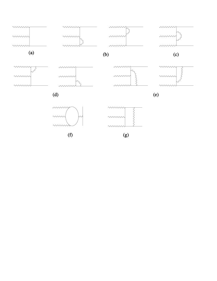
FIG. 1.: Feynman graphs contributing to the orthopositronium decay in the lowest order (a) and in the order-$\alpha$ radiative corrections (b-j). They are self-energy (b), inner vertex (c), outer vertex (d), double vertex (e), annihilation (f) and binding (g).

TABLE I.: Order-$\alpha$ radiative corrections to the decay matrix eigenvalues and change of eigenvectors rotation angle around decay plane normal due to radiative corrections.

		$-\frac{\Lambda_{i}-\Lambda^{0}_{i}}{\Lambda^{0}_{i}}\times 100$						$-\frac{\Lambda_{i}-\Lambda^{0}_{i}}{\Lambda^{0}_{i}}\times 100$
$\omega_{1}/m_{e}$	$\omega_{2}/m_{e}$	$i=1$	$i=2$	$i=3$	${\frac{\varphi-\varphi^{0}}{2},}^{\circ}$	$\omega_{1}/m_{e}$	$\omega_{2}/m_{e}$	$i=1$	$i=2$	$i=3$	${\frac{\varphi-\varphi^{0}}{2},}^{\circ}$
0.0323	0.9979	4.8	4.8	4.8	0.27	0.2906	0.9812	2.46	2.45	2.33	0.066
0.0344	0.9937	4.5	4.3	5.0	0.54	0.3094	0.9438	2.40	2.35	2.34	0.145
0.0365	0.9896	4.3	3.8	5.3	0.71	0.3281	0.9063	2.37	2.25	2.39	0.24
0.0385	0.9854	4.2	3.4	5.6	0.65	0.3469	0.8687	2.35	2.13	2.47	0.31
0.0406	0.9812	4.1	3.0	5.7	0.25	0.3656	0.8313	2.32	2.03	2.52	0.17
0.0969	0.9937	3.25	3.23	3.2	0.15	0.3552	0.9771	2.39	2.38	2.24	0.047
0.1031	0.9812	3.09	2.98	3.3	0.31	0.3781	0.9312	2.34	2.31	2.24	0.109
0.1094	0.9688	2.98	2.70	3.44	0.44	0.4010	0.8854	2.31	2.23	2.26	0.20
0.1156	0.9563	2.91	2.41	3.62	0.43	0.4240	0.8396	2.30	2.15	2.31	0.30
0.1219	0.9438	2.86	2.22	3.70	0.18	0.4469	0.7937	2.27	2.06	2.36	0.20
0.1615	0.9896	2.80	2.78	2.7	0.11	0.4198	0.9729	2.35	2.34	2.19	0.029
0.1719	0.9688	2.70	2.62	2.77	0.23	0.4469	0.9187	2.30	2.28	2.17	0.071
0.1823	0.9479	2.63	2.42	2.87	0.34	0.4740	0.8646	2.28	2.23	2.18	0.15
0.1927	0.9271	2.58	2.22	3.00	0.35	0.5010	0.8104	2.27	2.17	2.20	0.30
0.2031	0.9063	2.54	2.07	3.07	0.16	0.5281	0.7563	2.25	2.11	2.26	0.34
0.2260	0.9854	2.59	2.58	2.48	0.087	0.4844	0.9688	2.32	2.32	2.17	0.010
0.2406	0.9563	2.52	2.46	2.50	0.18	0.5156	0.9063	2.28	2.27	2.14	0.025
0.2552	0.9271	2.46	2.31	2.58	0.28	0.5469	0.8438	2.27	2.24	2.13	0.07
0.2698	0.8979	2.43	2.14	2.67	0.33	0.5781	0.7813	2.25	2.21	2.14	0.19
0.2844	0.8687	2.41	2.03	2.74	0.16	0.6094	0.7188	2.24	2.16	2.18	0.7

REFERENCES

- [1] J.S. Nico, D.W. Gidley, A. Rich and P.W. Zizewitz, Phys. Rev. Lett. 65, 1344 (1990).
- [2] J.S. Westbrook, D.W. Gidley, R.S. Conti, and A. Rich, Phys. Rev. A 40, 5849 (1989).
- [3] S. Asai, S. Orito, and N, Shinohara, Phys. Lett. B 357, 475 (1995).
- [4] V.G. Baryshevsky and O.N. Metelitsa, Acta Physica Polonica 88, 73 (1995).
- [5] M.A. Stroscio and J.M. Holt, Phys. Rev. A 10, 749 (1974).
- [6] W.E. Caswell, G.P. Lepage and J. Sapirstein, Phys. Rev. Lett. 38, 488 (1977).
- [7] W.E. Caswell and G.P. Lepage, Phys. Rev. A 20, 36 (1979).
- [8] G.S. Adkins, Annals of Physics 146, 78 (1983).
- [9] G.S. Adkins, A.A. Salahuddin and K.E. Schalm, Phys. Rev. A 45, 7774 (1992).
- [10] A.P. Burichenko, Yad. Fiz. 56, 123 (1993) [Phys. At. Nucl. 56, 640 (1993)].
- [11] G.S. Adkins, Phys. Rev. Lett. 76, 4903 (1996).
- [12] W. Bernreuther, U. Low and O. Nachtmann, Hyperfine Interactions 44, 139 (1988).
- [13] W. Bernreuther and O. Nachtmann, Z. Phys. C 11, 235 (1981); B.K. Arbic et al., Phys. Rev. A 37, 3189 (1988).
- [14] A.I. Akhiezer, V.B. Berestestkii Quantum Electrodynamics, Interscience Publishers, New York, London, Sydney, 1965.
- [15] V.B. Berestetskii, E.M. Lifshiz and L.P. Pitaevskii Quantum Electrodynamics, Landau and Lifshits Course of Theoretical Physics, vol. 4, New York, Pergamon, 1982.
- [16] R.P. Karplus, M. Neuman, Phys. Rev. 80, 380 (1950).
- [17] Y. Shima, Phys. Rev. 142, 944 (1966).