[

Numerical simulations of string networks in the Abelian-Higgs model

Abstract

We present the results of a field theory simulation of networks of strings in the Abelian Higgs model. Starting from a random initial configuration we show that the resulting vortex tangle approaches a self-similar regime in which the length density of lines of zeros of $\phi$ reduces as $t^{-2}$. We demonstrate that the network loses energy directly into scalar and gauge radiation. These results support a recent claim that particle production, and not gravitational radiation, is the dominant energy loss mechanism for cosmic strings. This means that cosmic strings in Grand Unified Theories are severely constrained by high energy cosmic ray fluxes: either they are ruled out, or an implausibly small fraction of their energy ends up in quarks and leptons.

]

In recent years, a sustained effort has gone into understanding the formation and evolution of networks of cosmic string, principally to provide a mechanism for seeding gravitational collapse [1, 2].

The picture that emerges from lattice simulations of string formation is a network consisting of a small number of horizon crossing self avoiding random walks, together with a scale invariant distribution of loops [3]. The subsequent evolution is driven by a tension in the strings causing them to straighten out. When two lengths of string pass through each other, they may intercommute, that is exchange partners. This allows the production of loops which can decay through gravitational radiation or particle production, depending on their size.

A number of numerical studies of network evolution have been carried out using the Nambu-Goto approximation of the string as a 1-dimensional object with a tension $\mu$. In particular we will refer later to work by Allen and Shellard (AS) and Bennett and Bouchet (BB), both reported in [4]. A consensus emerged from these studies that the network will relax into a scaling regime, where the large scale features of the network (the inter-string distance $\xi_{p}$ and the step length $\bar{\xi}_{p}$) grow with the horizon in proportion to $t$. On scales less than $\bar{\xi}_{p}$, there was evidence for a fractal substructure covering a range from the resolution scale to $\bar{\xi}_{p}$, which seems to be the result of kinks left behind by the production of loops. The loop production function itself did not scale: the distribution of loop sizes reported by BB is peaked around a cut-off introduced by hand into the simulation to ensure that even the smallest loops are approximated by a reasonable number of points.

It has been thought that the build-up of small scale structure will only be stopped by back-reaction from the string’s own gravitational field when the intermediate fractal extends to scales of order $G\mu\xi_{p}$, where $G$ is Newton’s constant. Then the small scale structure and loop production will scale with the horizon. Although much smaller than $\xi_{p}$, loops produced at this scale are still vastly bigger than the string core and will decay through gravitational radiation.

This picture has some support from a detailed analytical study by Austin, Copeland and Kibble [5] (ACK) which deals in part with length scales $\xi_{p}$, $\bar{\xi}_{p}$ and a scale $\zeta$, which can be interpreted as an angle-weighted average distance between kinks on the string. However, the ACK analysis relies on a number of unknown parameters, and for some parameter ranges small scale structure is absent.

In [6], Vincent, Hindmarsh and Sakellariadou (VHS) suggested a different picture based on results from Minkowski space Nambu-Goto simulations using the Smith-Vilenkin algorithm [7]. This algorithm is exact for string points defined on a lattice, allowing easy detection of intercommutation events. When loop production is unrestricted (up to the lattice spacing) they found that small scale structure disappeared, although loop production continued to occur at the lattice spacing. They could only recover the small scale structure seen in [4] by artificially restricting loop production with a minimum loop size greater than the lattice spacing. The suggestion is that the small scale structure seen in other simulations is an artifact of a minimum loop size and that loop production will occur at the smallest physical scale: the string width.

This has interesting consequences for energy loss from string networks. Loops formed at this size will decay into particles rather than gravitational radiation and could give a detectable flux [11]. If particle production provides the dominant energy loss channel, then GUT theories with strings are heavily constrained.

In this letter, we present the results of a series of field theory simulations of networks of Abelian Higgs vortices. They support the results of Vincent et al . If loops form, they form at the string width scale and promptly collapse. However, most of the string energy goes directly into oscillations of the field - radiation. We measure little small scale structure in the network. Furthermore, we find that the network scales with a scaling density consistent with the Smith-Vilenkin simulations, implying that the latter simulations do not unduly exaggerate energy loss as a lattice effect, a possibility suggested in [8].

The simplest gauge strings are contained in the Abelian-Higgs model, which has a Lagrangian

$${\mathcal{L}}=(D_{\mu}\phi)^{\dagger}(D^{\mu}\phi)-\frac{1}{4}F_{\mu\nu}F^{\mu\nu}-\frac{\lambda}{4}(|\phi|^{2}-\sigma^{2})^{2},$$ (1)

where $\phi$ is a complex scalar field, gauged by a U(1) vector potential with a covariant derivative $D_{\mu}=\partial_{\mu}-ieA_{\mu}$. $F_{\mu\nu}$ is the field strength tensor $\partial_{\mu}A_{\nu}-\partial_{\nu}A_{\mu}$. To model the system described by Eq. 1 we use techniques from hamiltonian lattice gauge theory [9] (and references therein).

An attractive feature of this formalism is that the Hamiltonian respects the discrete version of the $U(1)$ gauge transformations and consequently if Gauss’s law is true initially, then it is true for all later times. Significant violations of Gauss’s law are obtained if instead one uses a numerical scheme based on finite-differencing the Euler-Lagrange equations for $\phi$ and $A_{i}$.

The equations of motion derived from the Hamiltonian are evolved by discretising time with $\Delta t=ra$ ($r\ll 1$) and using the leapfrog method of updating field values on even time steps and the conjugate momentum on odd time steps. In keeping with the systems we are trying to model, we create initial conditions by allowing an energetic configuration of fields to dissipate energy until $\phi$ is close to the vacuum everywhere except near the string cores. We are not attempting to model the formation process, rather we wish to create a reasonable random network of flux vortices for subsequent evolution.

The simulation proceeds as follows. We generate a Gaussian random $k$-space configuration of each component of $\phi$ with a $k$-dependent Gaussian probability distribution with variance $\sigma_{\bf k}={\sqrt{m\;b}/{({\bf k}^{2}+m^{2}})}$. Samples drawn from this distribution are then Fourier transformed to $x$-space to generate a starting configuration, which will be uncorrelated on scales greater than $m^{-1}$. By varying the two paramenters $m$ and $b$ it is possible to control both the average amplitude and the correlation length of the initial configuration (this is in turn related to the initial defect density after the dissipation period). This then forms the initial conditions to be dissipated along with $\dot{\phi}=\theta^{i}=E^{i}=0$. Our dissipation scheme is to add the gauge invariant terms $\eta\pi_{x}$ and $\eta E_{x}^{i}$ to the equations of motion for $\phi$ and $\theta^{i}$. This ensures that Gauss’s law is preserved by the dissipation, but changes the charge-current continuity equation so that $\dot{\rho}+\nabla\cdot j=-\eta\rho.$ We have found that the most efficient dissipation is when the charge grows from $0$ to $e$ during the dissipation process. This allows the early formation of essentially global vortices, into which the magnetic flux relaxes as $e$ is increased.

Once the network has formed with $\langle{|\phi|\rangle}\approx 1$, we evolve the network with the dissipation turned off for half the box light-crossing time. During the evolution energy is conserved to within $\approx 0.3\%$.

A reasonable resolution of the string core is obviously an important requirement of the simulation. Traditionally the core is defined by the inverse masses of the field, so for $e=1$, $\lambda=2$ string, $d_{c}=1$. However, the fields depart appreciably from the vacuum over a larger distance, about 4 units.

We have performed a series of simulations on lattices of $224^{3}$, $304^{3}$ and $336^{3}$ points, lattice spacings of between $0.25$ and $0.75$, and with $r=0.15$. We vary the parameter $m$ in the variance of the field distribution to control initial defect density. In this letter we keep $\lambda/2e^{2}=1$.

Due to the size of the simulations we are unable to achieve the same level of statistical significance obtained using Nambu-Goto codes, although there are some revealing qualitative results.

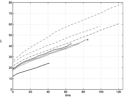
FIG. 1.: Plots of $\xi_{p}$ for a series of $336^{3}$ simulations with different lattice spacings. From top to botttom $a=$0.75, 0.65, 0.75, 0.4, 0.5, 0.45 and 0.25. In the initial gaussian distribution the parameter $m$ is varied to give the different initial correlation lengths. $\xi$ is given in units of the inverse scalar mass $m_{s}^{-1}$.

The gauge-invariant zero of the $\phi$ field provides a simple way of analysing the network of vortices. A string passes through a lattice cell face if the winding around the four corners is non-zero. By starting in any lattice cell with a string in it, the string can be followed around the lattice until it returns to the starting point. The distribution of box-crossing string and loops can then be analysed in much the same way as for Nambu-Goto strings [4, 6]. In particular, we are interested in the behaviour of the length scale $\xi_{p}$, roughly the inter-string distance, defined as $\xi_{p}={V/L^{2}_{\xi_{p}}}$, where $L_{\xi_{p}}$ is the total physical length of string above length $\xi_{p}$ (not the more usual invariant length). In practise, we calculate the length of string by smoothing over the string core width $d_{c}$. Scaling occurs if $\xi_{p}$ grows with $t$, although the actual value of $x_{p}$ in the scaling density $\rho_{\xi_{p}}={\mu/\xi_{p}^{2}}={\mu/x_{p}^{2}t^{2}}$, depends on the efficiency of the energy loss mechanism. Fig. 1 shows the function $\xi_{p}$ for a sample set of runs with different simulation parameters. Although with small dynamic ranges, one can never be sure that $\xi_{p}$ is approaching scaling or just on a slow transient, the scaling values for $x$ all appear to be in the range $0.27-0.34$, which is in agreement with Smith-Vilenkin simulations with maximum loop production where $x_{p}=0.27\pm 0.05$. This value is obtained by converting the invariant length $L_{\xi}$ used to define $\xi$ in [6] to physical length $L_{\xi_{p}}$, if $\bf X^{\prime}(\sigma)$ is the string tangent vector, then the physical length is just $L_{\xi_{p}}=\int d\sigma|\bf X^{\prime}|$. In the latter half of the simulation runs, these plots are extremely linear: the exponent of $t$ in $\xi\propto t^{p}$ is $p=1.002\pm 0.03$.

In [6], VHS argued that the string network is be dominated by processes on the smallest physical scale, either radiation or the production of loops at the string width. In all our runs performed so far, we find that this is true. When analysing the distribution of string formed by zeros of $\phi$, we consider three classes: long string ($L>\xi_{p}$), intermediate loops ($\pi d_{c}<L<\xi_{p}$) and core loops ($L<\pi d_{c}$). Fig. 2 shows a typical run for with a proportionate break down into types of loop over time.

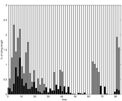
FIG. 2.: Proportion of string length intermediate loops (grey) and core loops (black). The long string (white) contribution makes up $100\%$. The lattice spacing is $a=0.35$.

Over the first part of the simulation we see an overall decrease in the percentage of string in loops of both types. Over the latter part of the simulation we see three sharp increases in $\%$ of intermediate loops at $t=37$, $t=61$ and $t=81$. In all three cases, this is caused by a single large loop (with $L>\xi_{p}$) decaying to below the $\xi_{p}$ threshold. Although these events constitutes a loss to the long string network, the decay channel is radiation and not an intercommutation event producing an intermediate loop. Note that aside from these loops, in the latter half of the simulation, all the string length is in long string (together with a small population of core loops), and the network continues to scale, despite some minor fluctuations in $\xi_{p}$ corresponding to the shrinking large loops (see curve marked ‘x’ in Fig. 1). We infer that all energy loss occurs ultimately through radiation and that it is very efficient at scaling the network.

To back up our claim that radiative processes are key to network evolution, we examined sinusoidal standing waves with wavelength $\lambda$ and initial amplitude $A$ where $A=\lambda/2$. The necessary scaling behaviour for the energy density in a network can be seen in the radiation from this system (incidentally one without intercommutation). Consider that a string network can be thought of as a length $\xi$ in a volume $\xi^{3}$, giving a density $\rho=\mu/\xi^{2}$ and $\dot{\rho}=-2\mu\dot{\xi}/\xi^{3}$. For a scaling network, $\dot{\rho}\xi^{3}=$ constant. We studied a series of standing waves with increasing wavlength $\lambda$ and measured the energy density $\rho(t)$ in a sub-volume $V_{\lambda}\sim\lambda^{3}$ around the string. We found that $\rho$ decays fairly linearly as the radiation from the string begins to leave $V_{\lambda}$, and then tails off as $A$ decreases significantly. We measure $\dot{\rho}$ during the linear region when $A\approx\lambda/2$. We find that $\dot{\rho}\lambda^{3}$ is constant to within 10 percent over a range of standing waves with $\lambda$ from 20 to 180, two orders of magnitude bigger than the string width. We also note that the pattern of oscillations around the standing wave remains substantially unchanged by an increase in the lattice spacing: we believe that any differences can be accounted for by the resulting decrease in resolution. The fact that the scaling density in the network simulation does not depend on the lattice spacing is also evidence that the radiative process is not a lattice artifact.

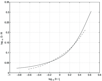
FIG. 3.: The fractal dimension of the long string at two times late in the evolution for $B=336^{3}$ and $a=0.75$ (solid), $a=0.25$ (dashed). The curves do not coincide, which may be due to difference in dynamic range in the two simulations.

It is claimed in [6] that if loop production is unrestricted, small scale structure will disappear. Small scale structure has been studied in two ways. Firstly, there is a length scale $\zeta$ mentioned in the introduction. Secondly, the relation between end-to-end distance $R$ and distance along the string $D$, $(D/R)\propto(D/\xi_{p})^{n},$ defines a scale-dependent fractal dimension $n$. If strings are smooth on small scales and brownian on large scales, $n$ should interpolate from $\sim 0$ to $\sim 0.5$. BB and AS observed that over a significant fraction of the range from the resolution scale to $\xi$, $n$ is constant. VHS showed from the behaviour of $\zeta$ that the region of constant $n$ did reflect the existence of small scale structure: when loop production is unrestricted the region of constant $n$ is absent and $\zeta\sim\xi$; when loop production is restricted a region of constant $n$ emerges and $\zeta\ll\xi$.

Fig. 3 shows that for the flux vortices $n$ varies smoothly from $\sim 0.01$ to $\sim 0.5$. The absence of the transient is in good qualitative agreement with the Nambu-Goto simulations with $\zeta\sim\xi$, and we can argue from this that gravitational radiation (gr) is irrelevant to our claimed particle production (pp). Energy loss processes can be described by an efficiency parameter $c$ in the rate equation $\dot{\rho}=-c\rho/\xi$. For a scaling network with $\zeta=\epsilon\xi$, $c_{{\rm gr}}=\Gamma G\mu/\epsilon$ where $\Gamma\sim 10^{1}-10^{2}$. If there is no small scale structure, $\epsilon\sim 1$ and, for GUT strings, $c_{{\rm gr}}=10^{-4}-10^{-5}$. This is to be compared with the overall energy loss through radiation in our simulations which gives $c_{{\rm pp}}=0.6$. It is only when there is considerable small scale structure ($\epsilon\sim 10^{-4}$) that gravitational radiation becomes significant.

We believe that our results support the claim of VHS that the dominant energy loss mechanism of a cosmic string network is particle production. Our field theory simulations show that the string network approaches self-similarity, as $\xi_{p}\propto t$, with a constant of proportionality $x_{p}$ consistent with Nambu-Goto codes which simulate string objects directly. We provide evidence that the long string network loses energy directly into oscillations of the field, which is the classical counterpart of particle production, or into loops of order the string width which quickly decay into particles. Previous calculations on particle production underestimated its importance by using perturbative calculations with light particles [10]. We see non-perturbative radiation at the string energy scale.

This represents a radical divergence from the traditional cosmic string scenario, which held that the loops are produced at scales much greater than the string width and subsequently decay by gravitational radiation. It implies that strong constraints come from the flux of ultra high energy (UHE) cosmic rays. Bhattacharjee and Rana [11] estimated that no more than about $10^{-3}$ of the energy of a GUT-scale string network can be injected as grand unified $X$ particles (assumed to decay into quarks and leptons). More recent calculations [12] limit the current energy injection rate $Q_{0}$ of particles of mass $m_{X}$ to approximately $Q_{0}\lesssim 2\times 10^{-34}(m_{X}/10^{15}\,{\rm GeV})^{0.44}{\rm\,ergs\,s}^{-1}{\rm cm}^{-3}$ (this formula is based on an eyeball fit to their most conservative bound in Fig. 2 [12]). Sigl et al [13] obtain somewhat lower values for $Q_{0}$: we have been cautious and adopted the higher value as our bound.

The energy injection rate from a scaling network is of order $\mu/t^{3}\sim 10^{-32}{\rm\,ergs\,s}^{-1}{\rm cm}^{-3}\,(\mu/10^{32}\,{\rm GeV}^{2}$). Taking $\mu\simeq 10m_{X}^{2}$, we derive $\mu\lesssim 10^{-29}f_{X}^{-1.3}\,{\rm GeV}^{2}$ or $G\mu\lesssim 10^{-9}f_{X}^{-1.3}$, where $f_{X}$ is the fraction of the energy appearing as quarks and leptons. Thus we conclude that GUT scale strings with $G\mu\sim 10^{-6}$ are ruled out: we regard a fraction $f_{X}\sim 5\times 10^{-3}$ as implausible.

We would like to thank Ray Protheroe, Hugh Shanahan and Günter Sigl for useful discussions, and Stuart Rankin for help with the UK-CCC facility in Cambridge. This research was conducted in cooperation with Silicon Graphics/Cray Research utilising the Origin 2000 supercomputer and supported by HEFCE and PPARC. GV and MH are supported by PPARC, by studentship number 94313367, Advanced Fellowship number B/93/AF/1642 and grant numbers GR/K55967 and GR/L12899. NDA is supported by J.N.I.C.T. - Programa Praxis XXI, under contract BD/2794/93-RM. Partial support is also obtained from the European Commission under the Human Capital and Mobility programme, contract no. CHRX-CT94-0423 and from the European Science Foundation.

REFERENCES

- [1] M. Hindmarsh and T.W.B. Kibble Rep. Prog. Phys. 58 477 (1994).
- [2] A. Vilenkin and E.P.S. Shellard, Cosmic Strings and other Topological Defects (Cambridge University Press, Cambridge, 1994).
- [3] T. Vachaspati and A. Vilenkin Phys. Rev. D30, 2036 (1984); T. W. B. Kibble Phys. Lett. 166B, 311 (1986); K. Strobl and M. Hindmarsh Phys. Rev. 1120 E55 (1997).
- [4] D. P. Bennett, in “Formation and Evolution of Cosmic Strings”, eds. G. Gibbons, S. Hawking and T. Vachaspati, (Cambridge University Press, Cambridge. 1990); F. R. Bouchet ibid.; E. P. S. Shellard and B. Allen ibid.
- [5] D. Austin, E. J. Copeland and T. W. B. Kibble Phys. Rev. D48 5594 (1993).
- [6] G. R. Vincent, M. Hindmarsh and M. Sakellariadou Phys. Rev. D56 637 (1997) .
- [7] A. G. Smith and A. Vilenkin Phys. Rev. D36 990 (1987).
- [8] A. Albrecht, in “Formation and Evolution of Cosmic Strings”, eds. G. Gibbons, S. Hawking and T. Vachaspati, (Cambridge University Press, Cambridge. 1990).
- [9] K. J. M. Moriarty, E. Myers and C. Rebbi Phys. Lett B207, 411 (1988). There are two typos in this paper. (i) The Wilson term for the gauge field in the Hamiltonian (Eq. 7) should have a factor in front. (ii) The equation of motion for the gauge field (Eq. 10b) is missing a factor of on the right hand side.
- [10] M. Srednicki and S. Theisen Phys. Lett. 189B 397 (1987); T. Vachaspati, A. E. Everett and A. Vilenkin Phys. Rev. D30 2046 (1984).
- [11] P. Bhattacharjee and N. C. Rana Phys. Lett. 246B 365 (1990).
- [12] R. J. Protheroe and T. Stanev Phys. Rev. Lett. 77 3708 (1996) [ E 78, 3420 (1997) ].
- [13] G. Sigl, S. Lee and P. Coppi, astro-ph/9604093.