NEW DEVELOPMENTS IN NON-HERMITIAN RANDOM MATRIX MODELS ^∗

${}^{\hbox{\scriptsize 1}}$Department of Physics, Jagellonian University, 30-059 Kraków, Poland
${}^{\hbox{\scriptsize 2}}$GSI, Planckstr. 1, D-64291 Darmstadt, Germany
${}^{\hbox{\scriptsize 3}}$Institut für Kernphysik, TH Darmstadt, D-64289 Darmstadt, Germany
${}^{\hbox{\scriptsize 4}}$Institute for Theoretical Physics, Eötvös University, Budapest, Hungary
${}^{\hbox{\scriptsize 5}}$Department of Physics, SUNY, Stony Brook, NY 11794, USA

INTRODUCTION

Random matrix models provide an interesting framework for modeling a number of physical phenomena, with applications ranging from atomic physics to quantum gravity ${}^{\hbox{\scriptsize\cite[cite]{[\@@bibref{}{WEIDNEW,ZINNJUSTIN}{}{}]}}}$. In recent years, non-hermitian random matrix models have become increasingly important in a number of quantum problems ${}^{\hbox{\scriptsize\cite[cite]{[\@@bibref{}{SOMMERSREV,UPDATENH}{}{}]}}}$. A variety of methods have been devised to calculate with random matrix models. Most prominent perhaps are the Schwinger-Dyson approach ${}^{\hbox{\scriptsize\cite[cite]{[\@@bibref{}{ZINNJUSTIN}{}{}]}}}$ and the supersymmetric method ${}^{\hbox{\scriptsize\cite[cite]{[\@@bibref{}{EFETOV}{}{}]}}}$. In the case of Non-hermitian Random Matrix Models (NHRMM) some of the standard techniques fail or are awkward.

In this talk we go over several new developments regarding the techniques ${}^{\hbox{\scriptsize\cite[cite]{[\@@bibref{}{NONHER,DIAG}{}{}]}}}$ for a large class of non-hermitian matrix models with unitary randomness (complex random numbers). In particular, we discuss
(a) - A diagrammatic approach based on a $1/N$ expansion
(b) - A generalization of the addition theorem (R-transformation)
(c) - A conformal transformation on the position of pertinent singularities
(d) - A ‘phase’ analysis using appropriate partition functions
(e) - A number of two-point functions and the issue of universality.

Throughout, we will rely on two standard examples: a non-hermitian gaussian random matrix model (Ginibre-Girko ensemble ${}^{\hbox{\scriptsize\cite[cite]{[\@@bibref{}{GINIBRE}{}{}]}}}$), and a chiral gaussian random matrix model in the presence of a constant non-hermitian part  ${}^{\hbox{\scriptsize\cite[cite]{[\@@bibref{}{STEPHANOV}{}{}]}}}$. The first ensemble being a text-book example will allow for a comparison of our methods to more conventional ones, the second ensemble will show the versatility of our approach to new problems with some emphasis on the physics issues. Further applications will be briefly mentioned.

DIAGRAMMATIC EXPANSION AND SPONTANEOUS BREAKDOWN OF HOLOMORPHY

The fundamental problem in random matrix theories is to find the distribution of eigenvalues in the large N (size of the matrix ${\cal M}$) limit. According to standard arguments, the eigenvalue distribution is easy to reconstruct from the discontinuities of the Green’s function

$$G(z)=\frac{1}{N}\left<{\rm Tr}\,\frac{1}{z-{\cal M}}\right>$$ (1)

where averaging is done over the ensemble of $N\times N$ random matrices generated with probability

$$P({\cal M})=\frac{1}{Z}e^{-N{\rm Tr}V({\cal M})}.$$ (2)

To illustrate our diagrammatic arguments let us first consider the well known case of a random hermitian ensemble with Gaussian distribution.

Hermitian diagrammatics

We use the diagrammatic notation introduced by ${}^{\hbox{\scriptsize\cite[cite]{[\@@bibref{}{BZ}{}{}]}}}$, borrowing on the standard large $N$ diagrammatics for QCD ${}^{\hbox{\scriptsize\cite[cite]{[\@@bibref{}{THOOFT}{}{}]}}}$. Consider the partition function

$$Z=<\det(z-H)>=\int d\psi d\psi^{\dagger}dHe^{-{\cal L}}e^{-\frac{N}{2}{\rm Tr}H^{2}}$$ (3)

with a “quark” Lagrangian ${\cal L}$

$${\cal L}=\bar{\psi}_{a}(z{\bf 1}_{a}^{b}-H^{b}_{a})\psi^{b}\,,$$ (4)

where $H$ is a hermitian random matrix with Gaussian weight ( the width of the Gaussian we set to 1). We will refer to $\psi$ as a “quark” and to $H$ as a “gluon”. The “Feynman graphs” following from (4) allow only for the flow of “color” (no momentum), since (4) defines a field-theory in $0+0$ dimensions. The names “quarks”, “gluons”, “color” etc. are used here in a figurative sense, without any connection to QCD. The “quark” and “gluon” propagators (double line notation) are shown in Fig. 1.

Figure 1.: Large $N$ “Feynman” rules for “quark” and “gluon” propagators.

Introducing the irreducible self energy $\Sigma$, the Green’s function reads

$$G(z)=\frac{1}{N}{\rm Tr}\,\frac{1}{z-\Sigma}=\frac{1}{z-\Sigma}\,.$$ (5)

In the large $N$ limit the equation for the self energy $\Sigma$ follows from resumming the rainbow diagrams of Fig. 2. All other diagrams (non-planar and “quark” loops) are subleading in the large $N$ limit. The consistency equation (“Schwinger-Dyson” equation of Fig. 3) reads

$$\Sigma=G.$$ (6)

Equations (5) and (6) give immediately $G(z-G)=1$, so the normalizable solution for the Green’s function reads

$$G(z)=\frac{1}{2}(z-\sqrt{z^{2}-4})$$ (7)

which, via the discontinuity (cut) leads to Wigner’s semicircle for the distribution of the eigenvalues for hermitian random matrices

$$\nu(\lambda)=\frac{1}{2\pi}\sqrt{4-\lambda^{2}}.$$ (8)

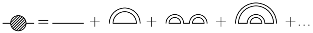
Figure 2.: Diagrammatic expansion of Green’s function (1) for Gaussian randomness.

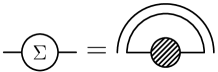
Figure 3.: Schwinger-Dyson equation.

Non-hermitian diagrammatics

If we were to use non-hermitian matrices in the resolvent (1), then configuration by configuration, the resolvent displays poles that are scattered around $z=0$ in the complex $z$-plane. In the large $N$ limit, the poles accumulate in general on finite surfaces (for unitary matrices on circles), over which the resolvent is no longer holomorphic. The (spontaneous) breaking of holomorphic symmetry follows from the large $N$ limit. As a result $\partial G/\partial\bar{z}\neq 0$ on the nonholomorphic surface, with a finite eigenvalue distribution. In this section we will set up the diagrammatic rules for investigating non-hermitian random matrix models. In addition to the “quarks” we introduce “conjugate quarks”, defined by the $0+0$ dimensional Lagrangian

$${\cal L}_{0}=\overline{\psi}(z-{\cal M})\psi+\overline{\phi}(\bar{z}-{\cal M}^{\dagger})\phi.$$ (9)

For hermitian matrices, “quarks” $\psi$ and “conjugate-quarks” $\phi$ decouple in the “thermodynamical” limit ($N\to\infty$). Their respective resolvents follow from (9) and do not ‘talk’ to each other. They are holomorphic (anti-holomorphic) functions modulo cuts on the real axis. For non-hermitian matrices, this is not the case in the large $N$ limit. The spontaneous breaking of holomorphic symmetry in the large $N$ limit may be probed in the $z$-plane by adding to (9)

$${\cal L}_{B}=\lambda(\overline{\psi}\phi+\overline{\phi}\psi)$$ (10)

in the limit $\lambda\longrightarrow 0$. The combination ${\cal L}_{0}+{\cal L}_{B}$ will be used below as the non-hermitian analog of the Lagrangian (4).

From (9,10) we define the matrix-valued resolvent through

$$\hat{{\cal{G}}}=\left(\begin{array}[]{cc}{\cal G}_{qq}&{\cal G}_{q\overline{q}}\\ {\cal G}_{\overline{q}q}&{\cal G}_{\overline{q}\overline{q}}\end{array}\right)=\left\langle\left(\begin{array}[]{cc}z-{\cal M}&\lambda\\ \lambda&\bar{z}-{\cal M}^{\dagger}\end{array}\right)^{-1}\right\rangle$$ (15)

where the limit $N\rightarrow\infty$ is understood before $\lambda\rightarrow 0$. The “quark” spectral density follows from Gauss law ${}^{\hbox{\scriptsize\cite[cite]{[\@@bibref{}{SOMMERS88}{}{}]}}}$,

$$\nu(z,\bar{z})=\frac{1}{\pi}\partial_{\bar{z}}\,\,G(z,\bar{z})=\frac{1}{\pi N}\partial_{\bar{z}}\,\,{\rm Tr}_{N}\,\,{\cal G}_{qq}$$ (16)

which is the distribution of eigenvalues of ${\cal M}$. For hermitian ${\cal M}$, (16) is valued on the real axis. As $\lambda\rightarrow 0$, the block-structure decouples, and we are left with the original resolvent. For $z\rightarrow+i0$, the latter is just a measurement of the real eigenvalue distribution, as shown before in the case of Gaussian hermitian ensemble. For non-hermitian ${\cal M}$, as $\lambda\rightarrow 0$, the block structure does not decouple, leading to a nonholomorphic resolvent for certain two-dimensional domains on the $z$-plane. Holomorphic separability of (9) is spontaneously broken in the large $N$ limit. For more technical details we refer to the original work ${}^{\hbox{\scriptsize\cite[cite]{[\@@bibref{}{DIAG}{}{}]}}}$. Similar construction has been proposed recently in  ${}^{\hbox{\scriptsize\cite[cite]{[\@@bibref{}{ZEENEW1}{}{}]}}}$.

Examples

Consider first the Ginibre-Girko ensemble, i.e. the case of complex matrices with the measure

$$<\ldots>=\int[d{\cal M}]\exp\left[-\frac{N}{(1-\tau^{2})}{\rm tr}({\cal M}{\cal M}^{\dagger}-\tau{\rm Re}{\cal M}{\cal M})\right]\,.$$ (17)

The “gluon” propagators read

$$\langle|{\cal M}_{ab}|^{2}\rangle=\frac{1}{N}\qquad\,\langle{\cal M}_{ab}{\cal M}_{ba}\rangle=\frac{\tau}{N}$$ (18)

corresponding to hermitian ($\tau=1$), anti-hermitian ($\tau=-1$) or general complex ($\tau=0$) matrix theory.

From (9,10) we note that there are two kinds of “quark” propagators ($1/z$ for “quarks” $\psi$ and $1/\bar{z}$ for “conjugate-quarks”$\phi$, where both can be incoming and outgoing). The relevant “gluonic” amplitudes correspond now to Fig. 4a–4d, where the (c,d) contribution corresponds to twisting the lines with a “penalty factor” $\tau$.

Figure 4.: All “gluonic” amplitudes for complex gaussian matrices.

The equation for the one particle irreducible (1PI) self-energy follows from Figs. 4–5 in the form

$$\left(\begin{array}[]{cc}\Sigma_{1}&\Sigma_{2}\\ \Sigma_{3}&\Sigma_{4}\end{array}\right) = \frac{1}{N}\mbox{\rm tr}\,_{N}\left(\begin{array}[]{cc}{\cal G}_{qq}&{\cal G}_{q\bar{q}}\\ {\cal G}_{\bar{q}q}&{\cal G}_{\bar{q}\bar{q}}\end{array}\right)\circ\left(\begin{array}[]{cc}\tau&1\\ 1&\tau\end{array}\right)$$ (25)

$$= \frac{1}{N}\mbox{\rm tr}\,_{N}\left(\begin{array}[]{cc}z-\Sigma_{1}&\lambda-\Sigma_{2}\\ \lambda-\Sigma_{3}&\bar{z}-\Sigma_{4}\end{array}\right)^{-1}\circ\left(\begin{array}[]{cc}\tau&1\\ 1&\tau\end{array}\right)\,.$$ (30)

Here the trace is meant component-wise (block per block), and the argument of the trace is the dressed propagator. The operation $\circ$ is not a matrix multiplication, but a simple multiplication between the entries in the corresponding positions. Here ${\rm tr}_{N}$ is short for the trace on the $N\times N$ block-matrices.

Each of the entries has a diagrammatical interpretation, in analogy to the hermitian case. For example, the equality for the upper left corners of matrices in (30) is represented diagrammatically on Fig. 5. The first graph on the r.h.s. in this figure does not influence the “quark-quark” interaction - it corresponds to the double line with a twist, therefore, as a non-planar one, is subleading. However, this twist could be compensated by the twisted part of the propagator coming from the second correlator (18), thereby explaining the factor $\tau$ in the upper left corner of (30). Other entries in (30) follow from Fig. 4 by inspection.

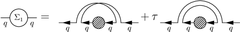
Figure 5.: Self-energy equation for non-hermitian matrices.

The “quark” one-point function is now

$$G(z,\bar{z})=\frac{1}{N}{\rm tr_{N}}\,\,{\cal G}_{qq}=({\bar{z}-\Sigma_{4}})/{det}\,.$$ (31)

It follows that $\Sigma_{2}=\Sigma_{3}$, with

$$det\cdot\Sigma_{1} = {\tau(\bar{z}-\Sigma_{4})}$$ (32)

$$det\cdot\Sigma_{4} = {\tau(z-\Sigma_{1})}$$ (33)

$$det\cdot\Sigma_{2} = \Sigma_{2}-\lambda\,,$$ (34)

where $det=(z-\Sigma_{1})(\bar{z}-\Sigma_{4})-(\lambda-\Sigma_{2})^{2}$. Substituting $r=\Sigma_{2}-\lambda$ in the last relation in (34) yields the equation

$$((z-\Sigma_{1})(\bar{z}-\Sigma_{4})-r^{2})(r+\lambda)=r\,.$$ (35)

For $\lambda=0$, the solution with $r=0$ is holomorphic while that with $r\neq 0$ is nonholomorphic. In the holomorphic case, $\Sigma_{1}(z-\Sigma_{1})=\tau$, and the resolvent is simply

$$G(z)=\frac{z\mp\sqrt{z^{2}-4\tau}}{2\tau}$$ (36)

where the upper sign corresponds to the solution with the pertinent asymptotics. In the nonholomorphic case, $G(z,\bar{z})=\bar{z}-\Sigma_{4}$, with

$$G(z,\bar{z})=\frac{\bar{z}-\tau z}{1-\tau^{2}}$$ (37)

in agreement with ${}^{\hbox{\scriptsize\cite[cite]{[\@@bibref{}{SOMMERS88}{}{}]}}}$. The boundary between the holomorphic and nonholomorphic solution follows from the condition $\Sigma_{2}=0$ imposed for the nonholomorphic solution, here this is equivalent to $|G(z,\bar{z})|^{2}=|G(z)|^{2}=1$, that is

$$\frac{x^{2}}{(1+\tau)^{2}}+\frac{y^{2}}{(1-\tau)^{2}}=1$$ (38)

which is an ellipse in the complex plane. Inside (38) the solution is nonholomorphic and outside it is holomorphic. The case investigated by Ginibre ${}^{\hbox{\scriptsize\cite[cite]{[\@@bibref{}{GINIBRE}{}{}]}}}$ follows for $\tau=0$. It is pedagogical to compare our method of solving this problem to the one coming from interpreting the Ginibre ensemble as a two-matrix (${\cal H}\sim H_{1}+iH_{2}$) model.

As a second example, we consider the Chiral Random Matrix model, which got recently some attention as a schematic model for spontaneous breakdown of the chiral symmetry. Here we consider for simplicity the Gaussian version of such model in the presence of a non-hermitian part, “chemical potential” $\mu$, as suggested by Stephanov ${}^{\hbox{\scriptsize\cite[cite]{[\@@bibref{}{STEPHANOV}{}{}]}}}$. The non-hermitian character comes from the property of Dirac matrices in Euclidean space. The form of the determinant stems from the constant mode sector of the massless and chiral Dirac operator at finite chemical potential ${}^{\hbox{\scriptsize\cite[cite]{[\@@bibref{}{MULAT}{}{}]}}}$. The corresponding partition function reads

$$Z=<\det(z-\mu\gamma-{\cal M})>$$ (39)

where

$$\gamma=i\gamma_{0}=\left(\begin{array}[]{cc}0&-1\\ 1&0\end{array}\right)\,\qquad{\rm and}\qquad{\cal M}=\left(\begin{array}[]{cc}0&H\\ H^{\dagger}&0\end{array}\right)\,.$$ (40)

The only novel features come from the “chiral character” of the matrix ${\cal M}$, i.e. the fact that it anticommutes with the $\gamma_{5}\equiv{\rm diag}({\bf 1}_{N},-{\bf 1}_{N})$. Due to this fact, the “gluon” propagator ${\cal D}$ inherits the block structure which in the tensor notation (see Fig. 1) reads

$${\cal D}=\frac{1}{N}(\gamma_{+}\otimes\gamma_{-}+\gamma_{-}\otimes\gamma_{+})$$ (41)

with $\gamma_{\pm}=({\bf 1}_{N}\pm\gamma_{5})/2$ and the bare “quark” propagator $1/z$ gets modified to $(z-\mu\gamma)^{-1}$. As a result, the 1PI self-energy equations in the planar approximation are given by

$$\left(\begin{array}[]{cc}\Sigma_{1}&\Sigma_{2}\\ \Sigma_{3}&\Sigma_{4}\end{array}\right)=\frac{1}{N}\mbox{\rm tr}\,_{N}\underbrace{\left(\begin{array}[]{cc}z-\mu\gamma-\Sigma_{1}&\lambda-\Sigma_{2}\\ \lambda-\Sigma_{3}&\bar{z}+\mu\gamma-\Sigma_{4}\end{array}\right)^{-1}}_{\mbox{\Large$\hat{{\cal G}}$}}\circ\left(\begin{array}[]{cc}{\cal D}&{\cal D}\\ {\cal D}&{\cal D}\end{array}\right)$$ (42)

where ${\cal D}$ is the “gluon” propagator (41), and $\Sigma_{i}$ are diagonal $2N\times 2N$ matrices. Inverting in (42) with respect to the “quark-conjugate quark” indices gives, after some elementary algebra, two kinds of solutions:

(i) A nonholomorphic solution ($\Sigma_{2}=\Sigma_{3}\neq 0$) ( “quark-quark” resolvent)

$$G(z,\bar{z})=\frac{1}{2N}\mbox{\rm tr}\,_{N}\ {\cal G}_{qq}=\frac{x}{2}-iy-\frac{1}{2}\frac{iy}{y^{2}-\mu^{2}}$$ (43)

where $z=x+iy$, a result first derived in ${}^{\hbox{\scriptsize\cite[cite]{[\@@bibref{}{STEPHANOV}{}{}]}}}$ using different arguments.

(ii) For $\Sigma_{2}=\Sigma_{3}=0$ we recover the holomorphic solution ${}^{\hbox{\scriptsize\cite[cite]{[\@@bibref{}{STEPHANOV,USMUX}{}{}]}}}$, $\Sigma_{1}(z)=G(z)\mbox{\bf 1}$, $\Sigma_{4}=\Sigma_{1}^{\dagger}$, with $G(z)$ fulfilling the cubic Pastur-like equation

$$G^{3}(z)-2zG^{2}(z)+(z^{2}+\mu^{2}+1)G(z)-z=0.$$ (44)

Note that in the case of this example the standard techniques of multi-matrix models do not apply.

ADDITION LAWS

The concept of addition law for hermitian ensembles was introduced in the seminal work by Voiculescu${}^{\hbox{\scriptsize\cite[cite]{[\@@bibref{}{VOICULESCU}{}{}]}}}$. In brief, Voiculescu proposed the additive transformation (R transformation), which linearizes the convolution of non-commutative matrices, alike the logarithm of the Fourier transformation for the convolution of arbitrary functions. This method is an important shortcut to obtain the equations for the Green’s functions for a sum of matrices, starting from the knowledge of the Green’s functions of individual ensembles of matrices. This formalism was reinterpreted diagrammatically by Zee ${}^{\hbox{\scriptsize\cite[cite]{[\@@bibref{}{ZEE}{}{}]}}}$, who introduced the concept of Blue’s function. Let us consider the problem of finding the Green’s function of a sum of two independent (free ${}^{\hbox{\scriptsize\cite[cite]{[\@@bibref{}{VOICULESCU}{}{}]}}}$) random matrices ${\cal M}_{1}$ and ${\cal M}_{2}$, provided we know the Green’s functions of each of them separately. First, we note that the 1PI self-energy $\Sigma$ can be always expressed as a function of $G$ itself and not of z as usually done in the textbooks. For the Gaussian randomness, $\Sigma_{H}(G)=G$ (see (6)). Second, we note that the graphs contributing to the self-energy $\Sigma_{1+2}(G)$ split into two classes, belonging to $\Sigma_{1}(G)$ and $\Sigma_{2}(G)$, due to the independence of probabilities $P(M_{1})$ and $P(M_{2})$ and large $N$ (planar) limit. Therefore

$$\Sigma_{1+2}(G)=\Sigma_{1}(G)+\Sigma_{1}(G).$$ (45)

Note that such a formula is not true if the energies are expressed as functions of $z$. Voiculescu R transformation is nothing but $R(u)\equiv\Sigma[G(u)]$. The addition (45) reads, for an arbitrary complex $u$, $R_{1+2}(u)=R_{1}(u)+R_{2}(u)$. The R operation forms and abelian group. The Blue’s function, introduced by Zee ${}^{\hbox{\scriptsize\cite[cite]{[\@@bibref{}{ZEE}{}{}]}}}$, is simply

$$B(G)=\Sigma(G)+G^{-1}.$$ (46)

Therefore, using the identity $G(z)=(z-\Sigma)^{-1}$, we see that the Blue’s function is the functional inverse of the Green’s function

$$B[G(z)]=z$$ (47)

and the addition law for Blue’s functions reads

$$B_{1+2}(z)=B_{1}(z)+B_{2}(z)-\frac{1}{z}.$$ (48)

The algorithm of addition is now surprisingly simple: Knowing $G_{1}$ and $G_{2}$, we find (47) $B_{1}$ and $B_{2}$. Then we find the sum $B_{1+2}$ using (48), and finally, get the answer $G_{1+2}$, by reapplying (47). Note that the method treats on equal footing the Gaussian and non-Gaussian ensembles, provided that the measures $P_{1}$ and $P_{2}$ are independent (free).

The naive extension of this algorithm fails completely for the non-hermitian matrices. It is not a priori puzzling - the underlying mathematical reason for (48) is the holomorphy of the hermitian Green’s function, not fulfilled for the case of NHRMM, as demonstrated in the previous section. However, since we managed to extend the diagrammatical analysis to the NHRMM, it is still possible to generalize the addition formula using the parallel diagrammatic reasoning like in the hermitian case. The generalization amounts to consider the matrix-valued Green’s function (15). The generalized Blue’s function ${}^{\hbox{\scriptsize\cite[cite]{[\@@bibref{}{NONHER,DIAG}{}{}]}}}$ is now a matrix valued function of a $2\times 2$ matrix variable defined by

$${\cal B}({\cal G})={\cal Z}=\left(\begin{array}[]{cc}z&\lambda\\ \lambda&\bar{z}\end{array}\right).$$ (51)

where $\lambda$ will be eventually set to zero. This is equivalent to the definition in terms of the self-energy matrix

$${\cal B}({\cal G})=\Sigma+{\cal G}^{-1}$$ (52)

where $\Sigma$ is a $2\times 2$ self energy matrix expressed as a function of a matrix valued Green’s function. The same diagrammatic reasoning as before leads to the addition formula for the self-energies and consequently for the addition law for generalized Blue’s functions

$${\cal Z}={\cal B}_{1}({\cal G})+{\cal B}_{2}({\cal G})-{\cal G}^{-1}.$$ (53)

The power of the addition law for NHRMM stems from the fact that it treats Gaussian and non-Gaussian randomness on the same footing ${}^{\hbox{\scriptsize\cite[cite]{[\@@bibref{}{ZEENEW2}{}{}]}}}$.

Example

Let us consider for simplicity complex random Gaussian matrices ($\tau=0$), which we rewrite as the sum $H_{1}+iH_{2}$, with $H_{1},H_{2}$ hermitian. The generalized Blue’s function for hermitian $H_{1}$ follows explicitly from

$$\Sigma^{(1)}\equiv\left(\begin{array}[]{cc}\Sigma^{(1)}_{1}&\Sigma^{(1)}_{2}\\ \Sigma^{(1)}_{3}&\Sigma^{(1)}_{4}\end{array}\right)=\hat{{\cal G}}\circ\left(\begin{array}[]{cc}1&1\\ 1&1\end{array}\right)=\hat{{\cal G}}$$ (58)

a matrix analog of (6). The generalized Blue’s function for anti-hermitian $iH_{2}$ follows from

$$\Sigma^{(2)}=\hat{{\cal G}}\circ\left(\begin{array}[]{rr}-1&1\\ 1&-1\end{array}\right)$$ (61)

where the entries reflect the antihermicity (set $\tau=-1$ in (30)). It is a straightforward exercise to check that the matrix equation (53) with the generalized Blue’s functions ${\cal B}_{1}$ and ${\cal B}_{2}$, corresponding to (58) and (61), reproduces two types of solutions (36) and (37) as well as the equation for the boundary ( here the circle) separating them on the $z$ plane.

CONFORMAL MAPPINGS

The existence of the nonholomorphic and as well holomorphic domains in the case of two solutions of NHRMM provides a powerful way to evaluate the supports for the level densities of NHRMM. The envelopes of these supports (supports form two-dimensional islands) can be derived very generally using a conformal transformation that maps the cuts of the hermitian ensemble onto the boundaries of its non-hermitian analog.

Let us consider the case where a Gaussian random and hermitian matrix $H$ is added to an arbitrary matrix $M$. The addition law says

$$R_{H+M}(u)=R_{H}(u)+R_{M}(u)=u+R_{M}(u).$$ (62)

where we have used explicitly that for Gaussian $R_{H}(u)=u$. Now, if we were to note that in the holomorphic domain the R transformation for the Gaussian anti-hermitian ensemble is $R_{iH}(u)=-u$, we read

$$R_{iH+M}(u)=R_{iH}(u)+R_{M}(u)=-u+R_{M}(u).$$ (63)

These two equations yield

$$B_{iH+M}(u)=B_{H+M}(u)-2u$$ (64)

where we have used the relation $B(u)=R(u)+1/u$. Substituting $u\rightarrow G_{H+M}(z)$ we can rewrite (64) as

$$B_{iH+M}[G_{H+M}(z)]=z-2G_{H+M}(z)\,.$$ (65)

Let $w$ be a point in the complex plane for which $G_{iH+M}(w)=G_{H+M}(z)$. Then

$$w=z-2G_{H+M}(z)\,.$$ (66)

Equation (66) provides a conformal transformation mapping the holomorphic domain of the ensemble $H+M$ (i.e. the complex plane $z$ minus cuts) onto the holomorphic domains of the ensemble $iH+M$, i.e. the complex plane $w$ minus the “islands”, defining in this way the support of the eigenvalues.

Examples

Consider the case of “summing” two Hermitian random Gaussian ensembles, i.e. consider the Hamiltonian $H=H_{H}+gH_{H}$, where $g$ is some arbitrary coupling. The sum constitutes of course the Gaussian ensemble, and the spectrum follows from the properties of the $R$ function $R_{H+gH}(z)=(1+g^{2})z$, or equivalently, Green’s function

$$G(z)=\frac{1}{2(1+g^{2})}[z-\sqrt{z^{2}-4(1+g^{2})}]$$ (67)

i.e. the support of the eigenvalues forms the interval (cut) ${\cal{I}}=[-2\sqrt{1+g^{2}},+2\sqrt{1+g^{2}}]$. According to (66), we can map the interval ${\cal{I}}$ onto the boundary delimiting the holomorphic domain of the non-hermitian ensemble ${\cal H}=H_{H}+i\gamma H_{H}$, ($g\rightarrow i\gamma$), that is

$$w=\frac{1}{1+g^{2}}[g^{2}z+\sqrt{z^{2}-4(1+g^{2})}]$$ (68)

with $z=t\pm i0$ and $t$ in ${\cal{I}}$. Equation (68) spans an ellipsis with axes $2/\sqrt{1+g^{2}}$ and $2g^{2}/\sqrt{1+g^{2}}$. For $g^{2}=1$ the ellipsis is just the Ginibre’s circle.

A similar construction and an identical mapping (66) gives the support of the eigenvalues in the case of a schematic chiral Dirac operator with chemical potential. Let us first consider the case when $\mu=i\epsilon$, i.e. the case when the ensemble is hermitian. In this case, the resulting Green’s function is known to fulfill the so-called Pastur equation (random gaussian plus deterministic hermitian Hamiltonian $E$, here with $N/2$ levels $\epsilon$ and $N/2$ levels $-\epsilon$)

$$G(z)=\frac{1}{z-G(z)-\epsilon}+\frac{1}{z-G(z)+\epsilon}$$ (69)

encountered in many areas of physics ${}^{\hbox{\scriptsize\cite[cite]{[\@@bibref{}{PASTUR}{}{}]}}}$. This is exactly equation (44) with the formal replacement $\mu^{2}\rightarrow-\epsilon^{2}$. At a particular value of the deterministic parameter $\epsilon=1$, the single cut supporting the spectrum of the hermitian ensemble splits into two-arc support, manifesting therefore a structural change in the spectral properties, hence a “phase transition”. The spectral properties of the non-hermitian model, with chemical potential $\mu$, follow from the mapping (66), but with $G_{H+M}$ replaced by an appropriate branch of the cubic Pastur equation (69). In particular, at the value $\mu^{2}=1$ the spectrum demonstrates the structural change - an island splits into two disconnected mirror islands (see Fig.6).

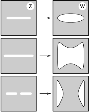
Figure 6.: Conformal mappings for the case of Ginibre-Girko ensemble with $\tau=0.5$ (upper), non-hermitian chiral ensemble with chemical potential $\mu^{2}=0.8$ (middle) and $\mu^{2}=1.2$ (lower). The shaded regions represent the holomorphic domains.

TWO-POINT FUNCTIONS

To probe the character of the correlations between the eigenvalues of non-hermitian random matrices, either on their holomorphic or nonholomorphic supports, it is relevant to investigate two-point functions. For example, a measure of the breaking of holomorphic symmetry in the eigenvalue distribution is given by the connected two-point function or correlator

$$N^{2}G_{c}(z,\bar{z})=\langle{\left|\mbox{\rm tr}\,\frac{1}{z-{\cal M}}\right|^{2}}\rangle_{c}$$ (70)

where the $z$ and $\bar{z}$ content of the averaging is probed simultaneously. The correlation function (70) will be shown to diverge precisely on the nonholomorphic support of the eigenvalue distribution, indicating an accumulation in the eigenvalue density. In the conventional language of “quarks” and “gluons”, (70) is just the correlation function between “quarks” and their “conjugates”. A divergence in (70) in the $z$-plane reflects large fluctuations between the eigenvalues of the non-hermitian operators on finite $z$-supports, hence their “condensation”.

It was shown in ${}^{\hbox{\scriptsize\cite[cite]{[\@@bibref{}{AMBJORN}{}{}]}}}$ and ${}^{\hbox{\scriptsize\cite[cite]{[\@@bibref{}{BREZIN}{}{}]}}}$ that for hermitian matrices (with $\bar{z}\to w$) the fluctuations in connected and smoothened two-point functions satisfy the general lore of macroscopic universality. This means that all smoothened correlation functions are universal and could be classified by the support of the spectral densities, independently of the specifics of the random ensemble and genera in the topological expansion (see ${}^{\hbox{\scriptsize\cite[cite]{[\@@bibref{}{AKEMANN}{}{}]}}}$ for a recent discussion).

In the case on NHRMM the generalized two-point correlator reads ${}^{\hbox{\scriptsize\cite[cite]{[\@@bibref{}{DIAG}{}{}]}}}$

$$N^{2}G_{c}(z,w)=-\partial_{z}\partial_{w}\log\det(1-{\cal G}_{1}\otimes{\cal G}_{2}^{T}\Gamma)\,.$$ (71)

Here the logarithm is understood as a power series expansion. Equation (71) is valid for Gaussian ensembles and, in the general case, up to factorizable corrections in the sense of ${}^{\hbox{\scriptsize\cite[cite]{[\@@bibref{}{BZ}{}{}]}}}$. The operator ${\cal G}_{1}\otimes{\cal G}_{2}^{T}\Gamma$ is a tensor product of $2\times 2$ matrices (see Fig. 7). The kernel $\Gamma$ includes the details of the “gluonic” interactions, depending on the particular measure. The tensor structure reflects the nonholomorphic solutions. The choice of “isospin” in the e.g. lower fermion line is done by choosing the appropriate derivative $\partial_{w}$ for the “quark” and $\partial_{\overline{w}}$ for the “conjugate-quark”.

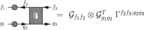
Figure 7.: Two-point kernel with $f,g=q,\bar{q}$.

For the holomorphic solutions of NHRMM, the structure is simpler, since the Green’s functions are holomorphic in this case.

Examples

In the case of the Ginibre Girko ensemble, the two-point correlator in the holomorphic domain reads simply

$$C(z,\bar{z})=-\partial_{z}\partial_{\bar{z}}\ln[1-G(z)G(\bar{z})]\,.$$ (72)

Indeed, in the holomorphic domain instead of the matrix valued ${\cal G}$ we use $G(z)$ given by (36), and the kernel $\Gamma$ reduces to the “quark-conjugate quark” coupling equal to 1 (upper-right corner of the last matrix in (30)). Note that the correlator (72) diverges on the line

$$1-|G(z)|^{2}=0$$ (73)

therefore the ellipse (38), confirming our statement.

For the nonholomorphic domain, the calculation is a bit more involved, due to the explicit matrix structure of ${\cal G}$ and $\Gamma$. The explicit form of the matrix-valued resolvent is

$${\cal G}=\frac{1}{1-\tau^{2}}\left(\begin{array}[]{cc}\bar{z}-\tau z&g_{z}\\ g_{z}&z-\tau\bar{z}\end{array}\right)$$ (76)

with $g_{z}^{2}=|z|^{2}(1-\tau)^{2}-\tau(z+\bar{z})^{2}-(1-\tau^{2})^{2}$. One recognizes (37) as the upper left corner of (76). The explicit form of the kernel is

$$\Gamma={\rm diag}(\tau,1,1,\tau)$$ (77)

which corresponds to all possible contributions from four graphs on Fig. 4. After some algebra, the determinant of 4 by 4 matrix $(1-{\cal G}_{1}\otimes{\cal G}_{2}^{T}\Gamma)$ turns out to be equal to $|z-w|^{2}$, giving the correlator

$$N^{2}G_{qq}(z,w) = -\frac{1}{(w-z)^{2}}\,.$$ (78)

In the non-hermitian chiral case the correlator in the outside (holomorphic) region is calculated using the same arguments as above. The only minor technical complication stems from the chiral (block) nature of the Green’s functions. We skip the details published elsewhere ${}^{\hbox{\scriptsize\cite[cite]{[\@@bibref{}{DIAG,USMUX}{}{}]}}}$, showing only the final result. The determinant of $1-{\cal G}_{1}\otimes{\cal G}_{2}^{T}\Gamma$ gives

$$\frac{(D-\mu^{2})^{2}-|z-G|^{4}}{D^{2}}$$ (79)

where the holomorphic G is the appropriate branch of (44) and $D=|(z-G)/G|^{2}$.

The zero of the determinant in (71) occurs for $(D-\mu^{2})=|z-G|^{2}$, that is

$$|z-G|^{2}(1-|G|^{2})-\mu^{2}|G|^{2}=0$$ (80)

as quoted in ${}^{\hbox{\scriptsize\cite[cite]{[\@@bibref{}{USMUX}{}{}]}}}$. This is exactly the equation of the boundary separating the holomorphic and nonholomorphic solutions, obtained in examples before either as $\Sigma_{2}=0$ or as a result of conformal mapping.

In the hermitian case $\mu=0$ (and $\bar{z}=w$), the determinant in (79) is simply $(1-G^{2}(z)G^{2}(w))$ (chiral) as opposed to $(1-G(z)G(w))$ (non-chiral). As a result, for $w=z$ and $\mu=0$, (79) is

$$N^{2}G(z,z)=\frac{1}{z^{2}(z^{2}-4)^{2}}$$ (81)

which coincides with (5.5) in ${}^{\hbox{\scriptsize\cite[cite]{[\@@bibref{}{MAKEENKO}{}{}]}}}$.

Note that the form of (81) signals two kinds of microscopic universalities. The $1/N$ expansion breaks down at $z=\pm 2$ (endpoints of spectra) and $z=0$ ( “Goldstone” pole due to the “chiral” nature of the ensemble).

The divergence at $z=\pm 2$ points at the edge universal behavior of the spectral function (Airy oscillations) ${}^{\hbox{\scriptsize\cite[cite]{[\@@bibref{}{AIRY}{}{}]}}}$, the divergence at $z=0$ signals the chiral microscopic universality ${}^{\hbox{\scriptsize\cite[cite]{[\@@bibref{}{BESSEL}{}{}]}}}$. Unfolding the spectra at these points allows to get the explicit universal kernels characterizing the fore mentioned universalities.

In the light of the above remarks, it is tempting to speculate ${}^{\hbox{\scriptsize\cite[cite]{[\@@bibref{}{DIAG}{}{}]}}}$, that the divergences of generalized correlators may onset some new types of microscopic universalities present in the NHRMM.

Note also that the relations (73), (79) demonstrating the functional dependence of the two-point correlator on one point holomorphic Green’s function allow for some extension of the macroscopic universality for NHRMM as well. The eventual geometric interpretation of this extension remains an open problem.

Before closing this example let us present for completeness the result of the chiral correlator in the nonholomorphic domain. The calculation is tedious, due to the fact that in the nonholomorphic region “quarks” may turn to “conjugate-quarks” and vice-versa, with all “quark” species interacting with themselves, and species appear in chiral copies. Nevertheless, the final result for the determinant is remarkably simple:

$$\det(1\!-\!{\cal G}(z)\otimes{\cal G}^{T}(w)\Gamma)=|z\!-\!w|^{2}|z\!+\!w|^{2}\frac{(\mu^{2}\!-\!(\mu^{2}\!-\!y^{2})(\mu^{2}\!-\!v^{2}))^{2}\!-\!v^{2}y^{2}}{\mu^{4}}\,$$ (82)

(where $y={\rm Im}\,z,v={\rm Im}\,w$), suggesting perhaps the possibility of further technical developments in the case of NHRMM.

PARTITION FUNCTIONS

We show now that the information carried by the one- and two-point functions is sufficient to specify the “thermodynamical” potential to order ${\cal O}(1/N)$ in the entire $z$-plane modulo isolated singularities, as we now discuss. Similar ideas were used in different context in ${}^{\hbox{\scriptsize\cite[cite]{[\@@bibref{}{STEELE,ITOI,AMBJORNETAL}{}{}]}}}$.

Let $Z_{N}$ be the partition function in the presence of an external parameter $z$. In the $1/N$ approximation, the diagrammatic contributions to the partition function $Z_{N}$ read

$$\log\,Z_{N}=NE_{0}+E_{1}+{\cal O}(\frac{1}{N})$$ (83)

where $E_{0}$ is the contribution of the “quark” or “conjugate quark” loop in the planar approximation, and $E_{1}$ is contribution of the “quark-quark” loop, and so on, in the same approximation. We will restrict our attention to non-hermitian matrices with unitary randomness, in which case the non-planar corrections to $E_{0}$ are of order $1/N^{2}$. Hence, $E_{0}$ is determined by the one-point function and $E_{1}$ by the two-point functions.

For $z$ such that (83) is real, continuous and nondecreasing function of the extensive parameters ${}^{\hbox{\scriptsize\cite[cite]{[\@@bibref{}{HUANG}{}{}]}}}$, $\log\,Z_{N}/N$ may be identified with the “pressure” of the random matrix model. As a result, the isolated singularities in the “pressure” are just the “phase” boundaries provided that the expansion is uniform. Below we give examples where the “phase” boundary is either mean-field-driven or fluctuation-driven. We have to distinguish two cases: holomorphic partition functions (“unquenched”) and nonholomorphic partition functions, where the complex phases of the determinants are neglected.

Holomorphic $Z$

We consider the partition function

$$Z_{N}=\langle{\det(z-{\cal M})}\rangle=\left<\int d\psi d\overline{\psi}e^{-\overline{\psi}(z-{\cal M})\psi}\right>\,.$$ (84)

In contrast to the one- and two-point correlators discussed above, the determinant in (84) is not singular in the $z$-plane configuration by configuration. Hence, (84) is a priori holomorphic in $z$ (minus isolated singularities).

The one- and two-point functions on their holomorphic support may be obtained from $\mbox{log}\,Z_{N}$ by differentiation with respect to $z$. Therefore, from (83)

$$E_{0}=\int^{z}\!dz^{\prime}\ G(z^{\prime})+const$$ (85)

or equivalently

$$E_{0}=zG-\int\!dG\ z(G)+const$$ (86)

after integrating by part. Note that $z(G)=B(G)$ is just the Blue’s function ${}^{\hbox{\scriptsize\cite[cite]{[\@@bibref{}{ZEE}{}{}]}}}$ of $G$. The constant in $E_{0}$ is fixed by the asymptotic behavior of (84), that is $Z_{N}\sim z^{N}$. The planar contribution to $E_{1}$ in (83) follows from the “quark-quark” wheel (two-point correlator). The final result for $Z_{N}$ is

$$Z_{N}=e^{NE_{0}}\cdot\left(\left\{\det(1-{\cal G}\otimes{\cal G}^{T}\cdot\Gamma)\right\}^{-\frac{1}{2}}+{\cal O}\left(\frac{1}{N}\right)\right)\,.$$ (87)

Note that due to the power $-1/2$, the fluctuations have “bosonic” character, and are dwarfed by the “quark” contribution as ($1:N$) ${}^{\hbox{\scriptsize\cite[cite]{[\@@bibref{}{USNJL}{}{}]}}}$. Both $E_{0}$ and $E_{1}$ are simple functions of the resolvent on a specific branch, as expected from generalized macroscopic universality.

We note that the partition function $Z_{N}$ through (87) exhibits an essential singularity in $1/N$ as expected from thermodynamical arguments. Assuming that the expansion for $\log Z_{N}/N$ is uniform, then $\log Z_{N}/N$ follows from (87) using the holomorphic resolvent $G(z)$ for large $z$. The small $z$ region follows by analytical continuation. However, since $G(z)$ is multi-valued (already the simple case of the Ginibre-Girko ensemble yields two branches for the resolvent in (36)), the analytical continuation is ambiguous. The ambiguity may be removed by identifying $\log|Z_{N}|/N$ with some generalized “pressure” and taking $G(z)$ so that $\log|Z_{N}|/N$ is maximum. As a result, $V_{N}=\log\,Z_{N}/N$ is piece-wise analytic in leading order in $1/N$ with “cusps” at

$$F^{(ij)}(x,y)\equiv V_{N}^{(i)}(x,y)-V_{N}^{(j)}(x,y)=0\,,$$ (88)

following the transition from branch $i$ to branch $j$ of $G$.

The character of the transition in the $1/N$ approximation can be highlighted by noting that for any finite $N$, the partition function (84) is a complex polynomial in $z$ of degree $N$ with random coefficients. In large $N$,

$$V_{N}=\frac{1}{N}\log\,|Z_{N}|=\frac{1}{2}\int\,dv\,d\overline{v}\,\varrho(v,\overline{v})\,\log|z-v|^{2}\,.$$ (89)

To leading order, the distribution of singularities along the “cusps” (88) is

$$\varrho(z,\bar{z})=\frac{1}{2\pi}|\partial_{z}F|^{2}\,\,\delta(F(z,\bar{z}))$$ (90)

which is normalized to 1 in the $z$-plane. Redefining the density of singularities by unit length along the curve $F(z,\bar{z})=0$, we may rewrite ( 90) as

$$\left.\varrho(z,\bar{z})\right|_{F=0}=\frac{1}{2\pi}|\partial_{z}F|\equiv\frac{1}{4\pi}|G^{(i)}-G^{(j)}|\,.$$ (91)

For $\varrho\neq 0$, the integrand in (89) is singular at $z=v$ which results into different forms for $V_{N}$, hence a cusp. For $\varrho=0$, that is $\partial_{z}F=0$, $V_{N}$ is differentiable. For physical $V_{N}$ (real and monotonically increasing), the points $\varrho=0$ are multi-critical points. At these points all $n$-point ($n\geq 2$) functions diverge. This observation also holds for Ising models with complex external parameters ${}^{\hbox{\scriptsize\cite[cite]{[\@@bibref{}{ROBERT}{}{}]}}}$. Assuming macroscopic universality ${}^{\hbox{\scriptsize\cite[cite]{[\@@bibref{}{AMBJORN}{}{}]}}}$ for all $n$-points ($n\geq 2$), we conclude that $\partial_{z}F=0$ means a branching point for the resolvents, hence $\partial_{z}G=\infty$ or $B^{\prime}(G)=0$ ${}^{\hbox{\scriptsize\cite[cite]{[\@@bibref{}{ZEE}{}{}]}}}$. For hermitian matrices, these conditions coincide with the end-points of the eigenvalue distributions ${}^{\hbox{\scriptsize\cite[cite]{[\@@bibref{}{ZEE,USBLUE}{}{}]}}}$.

Examples

To illustrate the above concepts, consider again first the Ginibre-Girko ensemble. The resolvent in the holomorphic region satisfies (36), so

$$z=\tau G+\frac{1}{G}\,.$$ (92)

The integration (86) in $E_{0}$ is straightforward, and after fixing the asymptotic behavior we obtain

$$Z_{N}=G^{-N}e^{\frac{\tau}{2}NG^{2}}\left((1-G^{2}(z)\tau)^{-\frac{1}{2}}+{\cal O}\left(\frac{1}{N}\right)\right)\,.$$ (93)

Here $G$ is the solution of (92). The pre-exponent in (93) follows from (87) with the matrix ${\cal G}$ replaced by $G$ and $\Gamma=\tau$, as seen in the “quark-quark” component of the vertex matrix in (30). Using (92) we observe that the pre-exponent diverges at two points in the $z$-plane, $z^{2}=4\tau$. At these points there is a “phase” change as we now show.

Given (93), the generalized “pressure” in leading order is

$$V_{\pm}=-\frac{1}{2}\mbox{log\,}(G_{\pm}\overline{G}_{\pm})+\frac{\tau}{4}(G_{\pm}^{2}+\overline{G}_{\pm}^{2})+{\cal O}\left(\frac{1}{N}\right)\,.$$ (94)

$V_{\pm}$ define two intersecting surfaces valued in the $z$-plane, for two branches $G_{\pm}$ of the solutions to (92). The parametric equation for the intersecting curve is

$$F(z,\bar{z})=V_{+}-V_{-}=0.$$ (95)

As indicated above, $V_{N}$ is piece-wise differentiable. Note that $F=0$ on the cut along the real axis, $-2\sqrt{\tau}<z<+2\sqrt{\tau}$, and from (91) the density of singularities per unit length is

$$\left.\varrho(z,\bar{z})\right|_{F=0}=\frac{1}{\pi}\frac{\sqrt{4\tau-z^{2}}}{2\tau}\,.$$ (96)

Along $F$, the density of singularities is semi-circle. The density (96) vanishes at the end-points $z=\pm 2\sqrt{\tau}$. This is easily seen to be the same as $\partial_{z}G=\infty$, or $dB(G)/dG=0$ with $B(G)=\tau G+1/G$. As noted above the term in bracket in Eq. (93) vanishes at these points, with a diverging “quark-quark” contribution. The transition is fluctuation-driven. These points may again signal the onset of scaling regions with possible universal microscopic behavior for non-hermitian random matrix models. This issue will be pursued elsewhere. At these points the $1/N$ expansion we have used breaks down.

Let us move now to the chiral non-hermitian ensemble. Elementary integration for this case leads to

$$Z_{N}(z,\mu)=e^{NE_{0}}\cdot\left(\left\{D^{-2}[(D+\mu^{2})^{2}-(z-G)^{4}]\right\}^{-\frac{1}{2}}+{\cal O}\left(\frac{1}{N}\right)\right)\,,$$ (97)

but now $D=(z-G)^{2}/G^{2}$, and

$$E_{0}(z,\zeta)=G^{2}+\log\frac{z-G}{G}$$ (98)

with the appropriate branch of holomorphic $G$ solution to (44).

Note that for $z=0$ and $G^{2}=-1-\mu^{2}$, the pre-exponent in (97) diverges. It also diverges at $z=z_{*}$ which are the zeros of (91) for the present case (two zeros for small $\mu$ and four zeros for large $\mu$), see Fig. 8. Again, at these points, the $1/N$ expansion breaks down marking the onset of scaling regions and the possibility of microscopic universality. The $z=0$ divergence is just the notorious “Goldstone” mode in chiral models, illustrating the noncommutativity of $N\rightarrow\infty$ and $z\rightarrow 0$. The rest of the arguments follow easily from the preceding example, in agreement with the “thermodynamics” discussed in ${}^{\hbox{\scriptsize\cite[cite]{[\@@bibref{}{USNJL}{}{}]}}}$. The analytical results for the nature and location of singularities of this example were confirmed by an extensive numerical analysis of Yang-Lee zeroes (up to 500 digits accuracy) in ${}^{\hbox{\scriptsize\cite[cite]{[\@@bibref{}{HALASZ}{}{}]}}}$.

Nonholomorphic $Z$

The above analysis for the holomorphic thermodynamical potential may also be extended to nonholomorphic partition functions of the type

$$Z_{N}[z,\bar{z}]=\langle{\det|z-{\cal M}|^{2}}\rangle=\left<\int d\psi d\overline{\psi}d\phi d\overline{\phi}e^{-\overline{\psi}(z-{\cal M})\psi-\overline{\phi}(\bar{z}-{\cal M}^{\dagger})\phi}\right>\,.$$ (99)

Note the important “quenching” of the phase of the determinant in comparison to the holomorphic case (84). As a consequence, the two-point correlators diverge rather on the one-dimensional boundary separating the phases (when approaching the boundary from the holomorphic domain) then at discrete points.

Similar reasoning as before leads to the explicit expression

$$Z_{N}[z,\bar{z}]\!\!=\!\!e^{NE_{0}}\cdot\left(\!\left\{\det(1\!\!-\!{\cal G}\otimes\overline{{\cal G}}^{T}\cdot\Gamma)\,|\!\det(1\!\!-\!{\cal G}\otimes{\cal G}^{T}\cdot\Gamma)|\right\}^{-1}\!\!\!+\!{\cal O}\!\left(\!\frac{1}{N}\!\right)\!\right)$$ (100)

where $E_{0}$ comes from the solutions of

$$G(z,\bar{z})=\frac{\partial E_{0}(z,\bar{z})}{\partial z}\qquad\overline{G}(z,\bar{z})=\frac{\partial E_{0}(z,\bar{z})}{\partial\bar{z}}\,.$$ (101)

Note that again the contributions from the two-wheel diagrams are of the form $1/\sqrt{{\rm det}}$ and hence “bosonic” in character. The result could be easily guessed without performing the calculations: there are two contributions from the “quark-conjugate-quark” wheels (correlators) (square of the $1/\sqrt{\det}$ in first term in the curly bracket) one contribution from the “quark-quark” wheel and one contribution from the “conjugate-quark-conjugate-quark” wheel (represented together as a second (modulus) term in the curly bracket).

Again, the partition function $Z_{N}$ has an essential singularity in $1/N$, but $\log Z_{N}/N$ does not. For any finite $N$, the latter diverges for

$$\det(1-{\cal G}\otimes\overline{{\cal G}}^{T}\cdot\Gamma)=0$$ (102)

which defines the line of singularities, and for

$$\det(1-{\cal G}\otimes{\cal G}^{T}\cdot\Gamma)=0$$ (103)

defining the set of discrete points, encountered in the case of the holomorphic partition function.

Examples

For the Ginibre-Girko example, the line of singularities (102) reads

$$1-|G|^{2}=0\,.$$ (104)

The line of singularities (104) reproduces in this case the ellipse (38). The ellipse includes the points of the “phase” change (see (93)),

$$1-\tau G^{2}(z)=0$$ (105)

i.e. the focal points $z^{2}=4\tau$, corresponding to (103), connected by the interval (95), i.e. $F=0$.

In the case of chiral non-hermitian random model the condition (102) reads ${}^{\hbox{\scriptsize\cite[cite]{[\@@bibref{}{USMUX}{}{}]}}}$

$$D^{-2}[(D-\mu^{2})^{2}-|z-G|^{4}]=0$$ (106)

with $D=|(z-G)/G|^{2}$, therefore exactly the condition (80). This line represents the boundary between the holomorphic and nonholomorphic solutions. The set of discrete multi-critical points, corresponding to (103) is given by the condition

$$D^{-2}[(D+\mu^{2})^{2}-(z-G)^{4}]=0$$ (107)

but with $D=[(z-G)/G]^{2}$, in agreement with (97). Note the crucial appearance of the modulus and the flip in the sign of $\mu$ when comparing last two formulae. The explicit solution of (107) consists on set of two or four points, (depending on the value of the $\mu$), being the analogs of Airy type end-points singularities and a single multi-critical point $z=0$, reflecting the chiral nature of the ensemble.

Figure 8 shows the critical lines and critical points corresponding to the conditions (102,103) for Ginibre-Girko and non-hermitian chiral ensembles. End-points singularities are denoted by “NATO stars”, chiral singularity – by “Zakopane sun”.

Figure 8.: Critical lines (102) and critical points (103) for Ginibre-Girko ensemble with $\tau=0.1$ (left) and non-hermitian chiral ensemble with small ($\mu^{2}=0.1$, middle) and large ($\mu^{2}=0.6$, right) value of chemical potential. The solid lines and the symbols represent the manifold on which the $1/N$ expansion breaks down and signal the location of possible microscopic universal behavior for NHRMM.

The fact that the critical line in Fig. 8 b,c surrounds the multi-critical points of the unquenched partition function, explains the failure of quenched lattice calculations with finite baryonic potential. The nature of chiral restoration is masked by unphysical fluctuations caused by neglecting the phase of the determinant. The critical line (106) exactly reproduces the shoreline of islands of unphysical “mixed-condensate”, obtained using the replica methods ${}^{\hbox{\scriptsize\cite[cite]{[\@@bibref{}{STEPHANOV}{}{}]}}}$.

CONCLUSIONS

Most of the details of results presented here are included in already published papers ${}^{\hbox{\scriptsize\cite[cite]{[\@@bibref{}{NONHER,DIAG,USMUX}{}{}]}}}$. In this mini-review on some novel aspects of NHRMM, we tried to enhance the role of a priori not obvious connections between the hermitian and non-hermitian ensembles of random matrices. In particular, we presented several ways for providing the supports and the density of eigenvalues for non-hermitian ensembles and the way for calculating smoothened (wide) correlations, via either analogies (diagrammatic expansion, generalized Blue’s functions), or formal relations between the hermitian and non-hermitian ensembles (conformal mapping, quenching/unquenching of partition function). We used the same set of known examples to demonstrate clearly the cross-references between the methods, as well to exhibit the shortcomings of the standard treatment.

We also speculated on some new features, like generalization of macroscopic universality and the possibility of several types of new microscopic universalities related to the critical behavior of various correlators in the NHRMM.

This last issue is of great interest in light of recent exciting results in “weakly” non-hermitian random matrix models ${}^{\hbox{\scriptsize\cite[cite]{[\@@bibref{}{WEAKLY}{}{}]}}}$ and related applications ${}^{\hbox{\scriptsize\cite[cite]{[\@@bibref{}{HATANONELSON}{}{}]}}}$.

Acknowledgments

This work was partially supported by the US DOE grant DE-FG-88ER40388, by the Polish Government Project (KBN) grant 2P03004412 and by Hungarian grants OTKA T022931 and FKFP0126/1997. MAN thanks the organizers of the Workshop for an opportunity to present this review and acknowledges interesting discussions with J. Ambjørn, J. Jurkiewicz, S. Nishigaki and J. Zinn-Justin.

REFERENCES

1. For a recent review, see T. Guhr, A. Müller-Gröling and H.A. Weidenmüller, e-print cond-mat/9707301.

2. P. Di Francesco, P. Ginsparg and J. Zinn-Justin, Phys. Rept. 254:1 (1995), and references therein.

3. Y. V. Fyodorov and H.-J. Sommers, J. Math. Phys. 38:1918 (1997), and references therein.

4. E. Brézin and A. Zee, e-print cond-mat/9708029, and references therein.

5. K.B. Efetov, Adv. in Phys. 32:53 (1983); J.J.M. Verbaarschot, H.A. Weidenmüller and M. R. Zirnbauer, Phys. Rep. 129:367 (1985).

6. R.A. Janik, M.A. Nowak, G. Papp, J. Wambach and I. Zahed, Phys. Rev. E55:4100 (1997)

7. R.A. Janik, M.A. Nowak, G. Papp and I. Zahed, Nucl. Phys. B501:603 (1997).

8. J. Ginibre, J. Math. Phys. 6:440 (1965); see also V.L. Girko, “Spectral Theory of Random Matrices” (in Russian), Nauka, Moscow, (1988).

9. M. Stephanov, Phys. Rev. Lett. 76:4472 (1996); M. Stephanov, Nucl. Phys. Proc. Suppl. 53:469 (1997).

10. E. Brézin and A. Zee, Phys. Rev. E49:2588 (1994); E. Brézin and A. Zee, Nucl. Phys. B453:531 (1995); E. Brézin, S. Hikami and A. Zee, Phys. Rev. E51:5442 (1995).

11. G. ’t Hooft, Nucl. Phys. B75:464 (1974).

12. J. Feinberg and A. Zee, e-print cond-mat/9703087.

13. H.-J. Sommers, A. Crisanti, H. Sompolinsky and Y. Stein, Phys. Rev. Lett. 60:1895 (1988).

14. I. Barbour et al., Nucl. Phys. B275:296 (1996); C.T.H. Davies and E.G. Klepfish, Phys. Lett. B256:68 (1991); J.B. Kogut, M.P. Lombardo and D.K. Sinclair, Phys. Rev. D51:1282 (1995).

15. R.A. Janik, M.A. Nowak, G. Papp and I. Zahed, Phys. Rev. Lett. 77:4876 (1996).

16. D.V. Voiculescu, Invent. Math. 104:201 (1991); D.V. Voiculescu, K.J. Dykema and A. Nica, “Free Random Variables”, Am. Math. Soc., Providence, RI, (1992); for new results see also A. Nica and R. Speicher, Amer. J. Math. 118:799 (1996) and references therein.

17. A. Zee, Nucl. Phys. B474:726 (1996).

18. J. Feinberg and A. Zee, e-print cond-mat/9704191.

19. L.A. Pastur, Theor. Mat. Phys. (USSR) 10:67 (1972); F. Wegner, Phys. Rev. B19:783 (1979); P. Neu and R. Speicher, J. Phys. A28:L79 (1995); E. Brézin, S. Hikami and A. Zee, Phys. Rev. E51:5442 (1995); A. D. Jackson and J.J.M. Verbaarschot, Phys. Rev. D53:7223 (1996); T. Wettig, A. Schäfer and H.A. Weidenmüller, Phys. Lett. B367:28 (1996); J. Jurkiewicz, M.A. Nowak and I. Zahed, Nucl. Phys. B478:605 (1996); M. Engelhardt, Nucl. Phys. B481:479 (1996).

20. J. Ambjørn, J. Jurkiewicz and Yu.M. Makeenko, Phys. Lett. B251:517 (1990).

21. E. Brézin and A. Zee, Nucl. Phys. B402:613 (1993).

22. G. Akemann and J. Ambjørn, J. Phys. A29:L555 (1996); G. Akemann, Nucl. Phys. B482:403 (1996); G. Akemann, e-print hep-th/9702005.

23. J. Ambjørn, C.F. Kristjansen and Yu.M. Makeenko, Mod. Phys. Lett. A7:3187 (1992).

24. M.J. Bowick and E. Brézin, Phys. Lett. B268:21 (1991).

25. E.V. Shuryak and J.J.M. Verbaarschot, Nucl. Phys. A560:306 (1993); J.J.M. Verbaarschot and I. Zahed, Phys. Rev. Lett. 70:3852 (1993); for recent results, see G. Akemann, P.H. Damgaard, U. Magnea and S. Nishigaki, Nucl. Phys. B487:721 (1997).

26. L. McLerran and A. Sen, Phys. Rev. D32:2795 (1985); T.H. Hansson and I. Zahed, Phys. Lett. B309:385 (1993); J.V. Steele, A. Subramanian and I. Zahed, Nucl. Phys. B452:545 (1995); J.V. Steele and I. Zahed, unpublished.

27. C. Itoi, Nucl. Phys. B493:651 (1997).

28. J. Ambjørn, L. Chekhov, C.F. Kristjansen and Yu. Makeenko, Nucl. Phys. B404:127 (1993).

29. K. Huang, “Statistical Mechanics”, John Wiley, New York, (1987).

30. M. A. Nowak, M. Rho and I. Zahed, “Chiral Nuclear Dynamics”, World Scientific, Singapore, (1996); R.A. Janik, M. A. Nowak, G. Papp and I. Zahed, Acta Phys. Pol. B27:3271 (1996); R.A. Janik, M. A. Nowak and I. Zahed, Phys. Lett. B392:155 (1997).

31. R. Schrock, private communication; G. Marchesini and R. Schrock, Nucl. Phys. B318:541 (1989); V. Matveev and R. Schrock, J. Phys. A28:1557 (1995); Nucl. Phys. Proc. Suppl. B42:776 (1995).

32. M.A. Nowak, G. Papp and I. Zahed, Phys. Lett. B389:137 (1996);

33. A. Halasz, A.D. Jackson and J.J.M. Verbaarschot, Phys. Lett. B395:293 (1997); A. Halasz, A.D. Jackson and J.J.M. Verbaarschot,e-print cond-mat/9703006.

34. Y.V. Fyodorov, B.A. Khoruzhenko and H.-J. Sommers, Phys. Lett. A226:46 (1997), and references therein; K. B. Efetov, e-print cond-mat/9702091.

35. N. Hatano and D.R. Nelson, Phys. Rev. Lett. 77:570 (1997); N. Hatano and D.R. Nelson, e-print cond-mat/9705290; J.T. Chalker and Z. Jane Wang, e-print cond-mat/9704198; J. Feinberg and A.Zee, e-print cond-mat/9706218; R.A. Janik, M.A. Nowak, G. Papp and I. Zahed, e-print cond-mat/9705098; P.W. Brouwer; P.G. Silvestrov and C.W.J. Beenakker, e-print cond-mat/9705186; I.Y. Goldsheid and B.A. Khoruzhenko, e-print cond-mat/9707230; see also ${}^{\hbox{\scriptsize\cite[cite]{[\@@bibref{}{UPDATENH}{}{}]}}}$.