Effective equation of state for a spherically expanding pion plasma

Abstract

Following a relativistic heavy ion collision, the quark-gluon plasma produced eventually undergoes a chiral phase transition. We assume that during this phase transition one can describe the dynamics of the system by the linear $\sigma$ model and that the expansion can be thought of as mostly radial. Because the $\sigma$ model is an effective field theory there is an actual momentum cutoff (Landau pole) in the theory at around 1 GeV. Thus it is necessary to find ways of obtaining a covariantly conserved, renormalized energy-momentum tensor when there is a cutoff present (which breaks covariance), in order to identify the effective equation of state of this time evolving system. We show how to solve this technical problem and then determine the energy density and pressure of the system as a function of the proper time. We consider different initial conditions and search for instabilities which can lead to the formation of disoriented chiral condensates (DCCs). We find that the energy density and pressure both decrease quickly, as is appropriate for a rapidly cooling system, and that the energy is numerically conserved.

I Introduction

During a relativistic heavy ion collision, it is possible to create a quark-gluon plasma, which will then cool and expand, leading to hadronization. At around the same time as hadronization, the system also undergoes a chiral phase transition which breaks the SU(2) $\times$ SU(2) symmetry and which then gives physical masses to the pion and other particles. The out of equilibrium dynamics of this phase transition can be very interesting if the expansion is fast enough so that the phase transition resembles a quench. In this case the effective pion mass can go negative for short periods of proper time which leads to a temporary exponential growth of low momentum domains where the isospin can point in a particular direction (DCC). This is a topic of current interest [1], since DCCs may provide a signature of the chiral phase transition. In an earlier paper [2] the time evolution of this chiral phase transition, assuming a uniform spherically symmetric expansion into the vacuum, was considered. The O(4) linear $\sigma$ model in the large-$N$ approximation, which incorporates both nonequilibrium and quantum effects, was studied. A range of initial conditions was analyzed to determine which initial states could lead to the formation of DCCs. This radial expansion is interesting because it is expected at late times in the plasma evolution, and also maximizes the cooling rate and therefore the possibility of the phase transition resembling a quench.

In this paper we go beyond previous work [2] and study the proper time evolutions of the effective hydrodynamic collective variables of the system, namely the renormalized pressure and energy density. We want to see to what extent previous intuition coming from studying classical hydrodynamical models of particle production such as Landau’s model is confirmed. This requires the solution of a new technical issue, namely how one obtains a covariantly conserved energy-momentum tensor when one has an actual cutoff in the theory. As discussed in earlier work [3, 13], the linear $\sigma$ model is an effective theory with a renormalized coupling constant of order 10, in order to agree with low energy pion properties. This leads to a maximum cutoff of around 1 GeV in order to avoid problems at scales of the order of the Landau pole. It has been shown earlier [3] that as long as the momentum cutoff determined from the sum over mode functions is below the Landau pole, there is a regime of cutoffs where the continuum renormalization group flow is obeyed so that one can safely say that one is in the continuum regime. For this class of problems, renormalization methods based on formal schemes such as dimensional regularization approaches are not very useful. Here we have a real cutoff in physical momentum as a result of using an effective field theory, and we have to be very careful in order to obtain the correct covariantly conserved energy-momentum tensor which leads to our definitions of comoving energy density and pressure variables. The tools we use to correctly renormalize the energy-momentum tensor are first to introduce the physical cutoff $\Lambda$ and then to analyze the divergences in all the components of the energy-momentum tensor using an adiabatic expansion of the mode functions. By comparing our results with a covariant point-splitting approach [4], we can identify those terms which should survive in the covariant limit. This technique allows us to obtain finite energy densities and pressures which then enable us to study the effective equation of state for the evolving plasma.

In this paper, we derive the energy-momentum tensor for the O(4) linear $\sigma$ model, and show how to regularize and renormalize it in order to obtain the physical energy density and pressure. We study initial conditions which have instabilities that lead to DCC formation and also stable initial configurations, and examine the energy density and pressure in both situations. We also consider the conservation of the energy-momentum tensor as a check on our numerical methods.

The paper is organized as follows. In Sec. II we discuss the model and coordinate system used, and show how to construct the energy-momentum tensor. Then in Sec. III we explicitly describe the scheme used to renormalize this tensor in order to perform a numerical simulation with a physical momentum cutoff. In Sec. IV we numerically examine the conservation of energy and the equation of state of the system. Finally in Sec. V we discuss the results and provide some concluding remarks.

II Energy-Momentum Tensor

A Equations of Motion and Coordinate System

We consider the O(4) linear $\sigma$ model, with the classical action given by [2]

$$S[\Phi_{i},\chi;j_{i}]=\int d^{4}x\sqrt{-g(x)}\left({\cal L}[\Phi_{i},\chi]+j_{i}\Phi_{i}\right)\>,$$ (1)

where the mesons are in a O(4) vector representation

$$\Phi_{i}=(\sigma,\vec{\pi})\>.$$ (2)

The Lagrangian density is

$${\cal L}[\Phi_{i},\chi]=\frac{1}{2}g_{\mu\nu}(x)[\partial^{\mu}\Phi_{i}(x)][\partial^{\nu}\Phi_{i}(x)]-\frac{1}{2}\chi(x)\Phi_{i}^{2}(x)+\frac{v^{2}}{2}\chi(x)+\frac{1}{4\lambda}\chi^{2}(x)\>.$$ (3)

In order to quantize the system, we construct the generating functional of the connected Green’s functions and carry out the path integral to obtain the following quantum effective action (to leading order in $N$) [2]

$$\Gamma[\phi_{i},\chi;j_{i}]=S[\phi_{i},\chi;j_{i}]+\frac{iN}{2}{\rm Tr}\ln G_{0}^{-1}(x,x^{\prime};\chi)\>,$$ (4)

where

$$G_{0}^{-1}(x,x^{\prime};\chi)=\left[\Box+\chi(x)\right]\delta^{4}(x,x^{\prime})/\sqrt{-g(x)}\>,$$ (5)

and

$$\phi_{i}(x) \equiv \langle\Phi_{i}(x)\rangle,$$ (6)

$$\chi(x) \equiv \langle\chi(x)\rangle\>.$$ (7)

By varying the effective action with respect to $\phi_{i}$ and $\chi$, we obtain the following equations of motion for the mean field $\phi_{i}$

$$\left[\Box+\chi(x)\right]\phi_{i}(x)=j_{i}(x)\equiv H\delta_{i0}\ \>,$$ (8)

and the constraint equation for the effective mass squared $\chi$

$$\chi(x)=\lambda[-v^{2}+\phi_{i}^{2}(x)-iNG_{0}(x,x;\chi)]\>.$$ (9)

Notice that $G_{0}(x,x^{\prime};\chi)$ depends on $\chi$ through its definition, and it fulfills the following dynamical equation

$$\left[\Box+\chi(x)\right]G_{0}(x,x^{\prime};\chi)=\delta^{4}(x,x^{\prime})/\sqrt{-g(x)}\>.$$ (10)

The current has only a non-vanishing component in the zero ($\sigma$) direction in order to give mass to the pion [2]. There are three parameters in the model: the mass of the pion $m=m_{\pi}$; the value of $H=f_{\pi}m_{\pi}^{2}$, which gives the vacuum expectation value $\langle\sigma\rangle=f_{\pi}$ (using PCAC); and the coupling constant $\lambda$, which is determined by fitting to low energy $\pi-\pi$ scattering data [2, 3].

The picture one gets from hydrodynamical simulations of heavy ion collisions is that the energy density is initially in a Lorentz contracted disk which expands first in the longitudinal direction and becomes three dimensional at late times. At early times one expects the velocity to scale approximately as $z/t$, where $z$ is the longitudinal direction, since the effective longitudinal size goes to zero with center of mass energy. This leads to the energy density approximately becoming a function only of the longitudinal fluid proper time variable $\tau_{z}=(t^{2}-z^{2})^{1/2}$. At later times when the expansion is more spherical and the initial distribution looks more like a “point”, one expects that the velocity scales as $v=r/t$ and the energy density then becomes a function of the spherical fluid variables:

$$\tau = {(t^{2}-r^{2})}^{1/2},$$ (11)

$$\eta = {\rm arctanh}(r/t)=\frac{1}{2}\ln\left(\frac{t+r}{t-r}\right)\>,$$ (12)

where $t=\tau\cosh\eta$ and $r=\tau\sinh\eta$ [5]. We restrict the range of these variables to the future light cone, namely $0\leq\tau<\infty$ and $0\leq\eta<\infty$. The coordinates $(\tau,\eta,\theta,\varphi)$ are useful to describe a spherically symmetric expansion of a plasma when one is in a hydrodynamical scaling regime. A spherical expansion provides the fastest possible expansion rate (and therefore cooling rate) of the quark-gluon plasma and thus enhances any nonequilibrium effects that are based on the idea of a rapid quench. Since complete inhomogeneous evolutions are at the edge of or beyond what is presently numerically possible, this spherically symmetric expansion provides the other extreme when compared with the slower, purely longitudinal expansion studied earlier [3].

In terms of this coordinate system, Minkowski’s line element

$$ds^{2}=dt^{2}-dr^{2}-r^{2}(d\theta^{2}+\sin^{2}\theta d\varphi^{2})$$ (13)

is given by

$$ds^{2}=d\tau^{2}-\tau^{2}(d\eta^{2}+\sinh^{2}\eta\;d\theta^{2}+\sinh^{2}\eta\sin^{2}\theta\;d\varphi^{2})\>,$$ (14)

from which we can read off the metric tensor

$$g_{\mu\nu}={\rm diag}\;(1,-\tau^{2},-\tau^{2}\sinh^{2}\eta,-\tau^{2}\sinh^{2}\eta\sin^{2}\theta)\>.$$ (15)

The metric in this coordinate system is of the Robertson-Walker form:

$$g_{\mu\nu}={\rm diag}\;(1,-{a^{2}(\tau)},-{a^{2}(\tau)}\sinh^{2}\eta,-{a^{2}(\tau)}\sinh^{2}\eta\sin^{2}\theta)\>,$$ (16)

which corresponds to a Ricci flat cosmological model with uniform expansion $a(\tau)=\tau$, and hyperbolic spatial sections, i.e., with curvature $\kappa=-1$.

It will be convenient to introduce the conformal time $u$ given by

$$u=\int^{\tau}a^{-1}(\tau^{\prime})\;d\tau^{\prime}\>,$$ (17)

or equivalently

$$\tau=\frac{{\rm e}^{u}}{m}\>,$$ (18)

where we choose $m=m_{\pi}$, the only mass scale in the system. The metric in the coordinate system with conformal time $(u,\eta,\theta,\varphi)$ has the form

$$g_{\mu\nu}=C(u)\;{\rm diag}\;(1,-1,-\sinh^{2}\eta,-\sinh^{2}\eta\sin^{2}\theta)\>,$$ (19)

with

$$C(u) = a^{2}(\tau)=\tau^{2}={\rm e}^{2u}/m^{2},$$ (20)

$$\sqrt{-g} = C^{2}(u)\sinh^{2}\eta\sin\theta\>.$$ (21)

In a hydrodynamical model, all the expectation values depend only on the proper time of the system. We therefore will assume that the mean fields $\phi_{i}$ and $\chi$ are only functions of $u$, that is $\phi_{i}=\phi_{i}(u)$ and $\chi=\chi(u)$. We then write the full quantum field $\Phi_{i}$ in terms of its expansion about its mean value, as follows:

$$\Phi_{i}(u,\eta,\theta,\phi)=\phi_{i}(u)+\hat{\phi}_{i}(u,\eta,\theta,\phi),$$ (22)

where $\hat{\phi}_{i}$ are the quantum fluctuations, which include both vacuum and thermal excitations. The equations of motion are then

$$\left[C^{-1}(u)\left(\frac{{\partial}^{2}}{\partial u^{2}}+2\frac{\partial}{\partial u}\right)+\chi(u)\right]\phi_{i}(u) = H\delta_{i0},$$ (23)

$$\left[\Box+\chi(u)\right]\hat{\phi}_{i}(x) = 0\>,$$ (24)

where $x$ is the four vector $x=(u,\eta,\theta,\varphi)$. Then for $G_{0}(x,x^{\prime};\chi)$ we find

$$G_{0}(x,x^{\prime};\chi)=i\;\langle{\rm T}_{c}\{\hat{\phi}_{i}(x),\hat{\phi}_{i}(x^{\prime})\}\rangle\>,$$

where T_c corresponds to a $u$-ordered product, following the closed-time-path formalism of Schwinger [6].

In order to solve the wave equation for the quantum fluctuations, we follow Parker and Fulling [7], and write a mode expansion for $\hat{\phi}_{i}$ as follows

$$\hat{\phi}_{i}(u,\vec{x})=C^{-1/2}(u)\;\int_{0}^{\infty}ds\sum_{lm}\bigl{[}\hat{a}_{i,slm}\,g_{s}(u){\cal{Y}}_{slm}(\vec{x})+{{\hat{a}}^{{\dagger}}}_{i,slm}\,{g_{s}^{*}}(u){\cal{Y}}^{\ast}_{slm}(\vec{x})\bigr{]}\>,$$ (25)

with

$$\vec{x}=(\eta,\theta,\phi),$$

and

$$\Delta^{(3)}{\cal Y}_{slm}(\vec{x})+(s^{2}+1){\cal Y}_{slm}({\vec{x}})=0\>,$$

where $\Delta^{(3)}$ is the Laplacian of the three dimensional hyperbolic spatial sections of curvature $\kappa=-1$. Then the mode functions $g_{s}(u)$ satisfy the following differential equation

$${\ddot{g}}_{s}(u)+\left[s^{2}+C(u)\chi(u)\right]g_{s}(u)=0\>,$$ (26)

and for $G_{0}(x,x;\chi)$ we find [2]

$$\langle\hat{\phi}_{i}^{2}\rangle=-i\;G_{0}(x,x;\chi)=C^{-1}(u)\int_{0}^{\infty}\,\frac{s^{2}ds}{2{\pi^{2}}}(2n_{s}+1)|g_{s}(u)|^{2}\>,$$ (27)

once we have chosen a particular vector state with respect to which we shall be taking expectation values. We choose an initial state such that the pair densities are zero, and the particle number density is finitely integrable with respect to the corresponding integration measure, namely

$$\langle\hat{a}_{j,s^{\prime}l^{\prime}m^{\prime}}^{\dagger}\hat{a}_{i,slm}\rangle = n_{s}\,\delta_{ij}\,\delta(s^{\prime}-s)\,\delta_{ll^{\prime}}\,\delta_{mm^{\prime}}\>,$$

$$\langle\hat{a}_{j,s^{\prime}l^{\prime}m^{\prime}}\hat{a}_{i,slm}^{\dagger}\rangle = (n_{s}+1)\,\delta_{ij}\,\delta(s^{\prime}-s)\,\delta_{ll^{\prime}}\,\delta_{mm^{\prime}}\>,$$

$$\langle{{\hat{a}}^{{\dagger}}}_{i,slm}{{\hat{a}}^{{\dagger}}}_{j,s^{\prime}l^{\prime}m^{\prime}}\rangle = p_{s}\,\delta_{ij}\,\delta(s^{\prime}-s)\,\delta_{ll^{\prime}}\,\delta_{mm^{\prime}}=0\>,$$

$$\langle{{\hat{a}}}_{i,slm}{{\hat{a}}}_{j,s^{\prime}l^{\prime}m^{\prime}}\rangle = p_{s}^{\ast}\,\delta_{ij}\,\delta(s^{\prime}-s)\,\delta_{ll^{\prime}}\,\delta_{mm^{\prime}}=0\>.$$

Here we choose the initial particle number density to be a thermal distribution

$$n_{s}=[e^{\omega_{s}(u_{0})/k_{B}T}-1]^{-1}\>,$$

where ${{\omega}^{2}_{s}(u_{0})}=s^{2}+C(u_{0})\chi(u_{0})$. Notice that we can choose the pair density to vanish $(p_{s}=0)$, since one has the freedom to make a Bogoliubov transformation at $u_{0}$ so that this always remains true. The boundary conditions on the mode functions $g_{s}(u)$ is that they correspond to the positive frequency adiabatic mode functions initially. We therefore choose

$$g_{s}(u_{0}) = 1/\sqrt{2\omega_{s}(u_{0})},$$ (28)

$$\dot{g}_{s}(u_{0}) = -\left\{\frac{\dot{\omega}_{s}(u_{0})}{2\omega_{s}(u_{0})}+i\omega_{s}(u_{0})\right\}g_{s}(u_{0})\>.$$ (29)

The following rescalings will be useful:

$$\phi_{i}(u)=C^{-1/2}(u)\rho_{i}(u),$$ (31)

$$\chi(u)=C^{-1}(u)\tilde{\chi}(u),$$ (32)

$$j_{i}=C^{-3/2}(u)\tilde{j}_{i}(u),$$ (33)

$$v=C^{-1/2}(u)\tilde{v}(u)\>.$$ (34)

In terms of the scaled variables, the equations of motion can be written

$$\left[\frac{d^{2}}{du^{2}}+s^{2}+\tilde{\chi}(u)\right]g_{s}(u) = 0,$$ (35)

$$\left[\frac{d^{2}}{du^{2}}-1+\tilde{\chi}(u)\right]\rho_{i}(u) = \tilde{j}_{i}(u)\>,$$ (36)

with the gap equation being

$$\frac{\tilde{\chi}(u)}{\lambda}=-{\tilde{v}}^{2}(u)+\rho^{2}_{i}(u)+N\int_{0}^{\infty}\,\frac{s^{2}ds}{2{\pi^{2}}}(2n_{s}+1)|g_{s}(u)|^{2}\>.$$ (37)

B Construction of the Stress-Energy Tensor

The energy-momentum tensor is defined by [8]

$$T_{\mu\nu} = (1-2\xi)(\nabla_{\mu}\Phi_{i})\,(\nabla_{\nu}\Phi_{i})+\left(2\xi-\frac{1}{2}\right)g_{\mu\nu}g^{\alpha\beta}(\nabla_{\alpha}\Phi_{i})\,(\nabla_{\beta}\Phi_{i})$$ (38)

$$- 2\xi\Phi_{i}(\nabla_{\mu}\nabla_{\nu}\Phi_{i})+\frac{1}{2}\xi g_{\mu\nu}\Phi_{i}\Box\Phi_{i}+\frac{1}{2}(1-3\xi)\chi g_{\mu\nu}\Phi_{i}^{2}$$ (39)

$$- g_{\mu\nu}\frac{\chi v^{2}}{2}-g_{\mu\nu}\frac{\chi^{2}}{4\lambda}-g_{\mu\nu}\left(1-\frac{3\xi}{2}\right)j_{i}\Phi_{i}\>.$$ (40)

Equivalently, we can write this equation as [9]

$$T_{\mu\nu}=(\nabla_{\mu}\Phi_{i})\,(\nabla_{\nu}\Phi_{i})+\xi(g_{\mu\nu}\Box-\nabla_{\mu}\nabla_{\nu})\Phi_{i}^{2}-g_{\mu\nu}\left({\cal L}[\Phi_{i},\chi]+j_{i}\Phi_{i}\right)\>,$$ (41)

where ${\cal L}[\Phi_{i},\chi]$ is given by Eq. (3). We take the expectation value of the energy-momentum tensor in the thermal initial state chosen, and make use of the mode expansion given in Eq. (25) to examine the components of $T_{\mu\nu}$.

After some algebra, we find for the $T_{uu}$ component

$$C(u)\langle{T}_{uu}\rangle = \frac{1}{2}\left[\dot{\rho}_{i}^{2}+(\tilde{\chi}+1-12\xi)\,\rho_{i}^{2}\right]$$ (45)

$$+(6\xi-1)\rho_{i}\dot{\rho}_{i}-\tilde{j}_{i}\rho_{i}-\frac{\tilde{\chi}\tilde{v}^{2}}{2}-\frac{\tilde{\chi}^{2}}{4\lambda}$$

$$+\frac{N}{2}\int_{0}^{\infty}\frac{s^{2}ds}{2\pi^{2}}(2n_{s}+1)\Biggl{\{}\left|\dot{g_{s}}\right|^{2}+(s^{2}+\tilde{\chi}+2-12\xi)\,|g_{s}|^{2}$$

$$+(6\xi-1)(g_{s}\dot{g_{s}^{\ast}}+g_{s}^{\ast}\dot{g_{s}})\Biggr{\}}\>,$$

and similarly for the $T_{\eta\eta}$ component

$$C(u)\langle{T}_{\eta\eta}\rangle = \frac{1}{2}\left[\dot{\rho}_{i}^{2}(1-4\xi)+(1-\tilde{\chi}-8\xi+4\xi\tilde{\chi})\,\rho_{i}^{2}\right]$$ (50)

$$+(6\xi-1)\rho_{i}\dot{\rho_{i}}+(1-2\xi)\tilde{j}_{i}\rho_{i}+\frac{\tilde{\chi}\tilde{v}^{2}}{2}+\frac{{\tilde{\chi}}^{2}}{4\lambda}$$

$$+\frac{N}{2}\int_{0}^{\infty}\frac{s^{2}ds}{2\pi^{2}}(2n_{s}+1)\Biggl{\{}(1-4\xi)\left|\dot{g_{s}}\right|^{2}$$

$$+\left[-\frac{s^{2}}{3}-\tilde{\chi}+\frac{2}{3}+4\xi(s^{2}+\tilde{\chi}-1)\right]\,|g_{s}|^{2}$$

$$+(6\xi-1)(g_{s}\dot{g_{s}^{\ast}}+g_{s}^{\ast}\dot{g_{s}})\Biggr{\}}\>.$$

It can be easily shown that the energy-momentum tensor is diagonal and that the spatial components are all equal, except for a geometrical factor (see Appendix B). We then define [5]

$$\langle\,T_{\mu\nu}\,\rangle\equiv C(u){\rm diag}\,(\,\epsilon,\,p,\,p\,\sinh^{2}\eta,\,p\,\sinh^{2}\eta\sin^{2}\theta\,)\>.$$ (51)

III Renormalization of $T_{\mu\nu}$

In order to analyze the divergences of $\langle T_{\mu\nu}\rangle$ we make use of the adiabatic expansion of the modes $g_{s}$, since we know [10] that ${\langle T_{\mu\nu}\rangle}$ and ${\langle T_{\mu\nu}\rangle}_{\rm adiabatic}$ have the same ultraviolet behaviour. Up to second adiabatic order we have [10]

$$g_{s}^{A}=\frac{1}{\sqrt{2\Omega_{s}}}\;{\rm exp}\left[-i\int^{u}du^{\prime}\Omega_{s}(u^{\prime})\right],$$ (53)

$$|g_{s}^{A}|^{2}=\frac{1}{2\Omega_{s}}=\frac{1}{2\omega_{s}}+\frac{\ddot{\omega}_{s}}{8\omega_{s}^{4}}-\frac{3\dot{\omega}_{s}^{2}}{16\omega_{s}^{5}}+\cdots,$$ (54)

$$|\dot{g}_{s}^{A}|^{2}=\frac{1}{2\Omega_{s}}\left(\frac{\dot{\Omega}_{s}^{2}}{4\Omega_{s}^{2}}+\Omega_{s}^{2}\right)=\frac{\omega_{s}}{2}-\frac{\ddot{\omega}_{s}}{8\omega_{s}^{2}}+\frac{5\dot{\omega}_{s}^{2}}{16\omega_{s}^{3}}+\cdots,$$ (55)

$$(g_{s}^{A}\dot{g}_{s}^{A\ast}+\dot{g}_{s}^{A}g_{s}^{A\ast})=-\frac{1}{2}\frac{\dot{\Omega}_{s}}{\Omega_{s}^{2}}=-\frac{1}{2}\frac{\dot{\omega}_{s}}{\omega_{s}^{2}}+\cdots\>,$$ (56)

where $\omega_{s}^{2}(u)=s^{2}+\tilde{\chi}(u)$.

We regularize our integrals by introducing a non-covariant cutoff $\Lambda$ in physical momentum, which corresponds to a comoving momentum cutoff $s_{m}=C^{1/2}(u)\Lambda$. We shall work with a fixed physical cutoff $\Lambda$, so that the comoving cutoff $s_{m}$ depends on the conformal time $u$.

We have three physical parameters to renormalize: the mass of the pion $m_{\pi}$, the self-interaction coupling constant $\lambda$, and the (dimensionless) coupling constant to gravity $\xi$, necessary in order for the field theory to be renormalizable, even in Ricci flat spacetimes, such as the one considered in this paper [11]. The quadratic divergences in the gap equation will be removed by mass renormalization, and the logarithmic divergences will be subtracted by renormalization of the coupling constants $\lambda$ and $\xi$. In addition, we shall see that there is an extra quartic divergence in both the energy density and the pressure, coming from the mode integrals in ${\langle T_{\mu\nu}\rangle}$ that carry an extra factor of $k^{2}$, which can be removed by renormalizing the cosmological constant.

First we examine the divergences in the gap equation (37). From the adiabatic expansion (III), we know that the mode integral appearing in this equation has a quadratic divergence. In order to remove this divergence, we perform mass renormalization by subtracting the regularized gap equation for the vacuum state:

$$\frac{C(u)m^{2}}{\lambda}=-{\tilde{v}}^{2}(u)+C(u)f_{\pi}^{2}+\frac{N}{2}\int_{0}^{s_{m}}\,\frac{s^{2}ds}{2{\pi^{2}}}\frac{1}{{(s^{2}+{\rm e}^{2u})}^{1/2}}\>.$$ (57)

This yields for the gap equation

$$\frac{\tilde{\chi}(u)}{\lambda}=\frac{C(u)m^{2}}{\lambda}+\rho_{i}^{2}(u)-C(u)f_{\pi}^{2}+N\int_{0}^{s_{m}}\,\frac{s^{2}ds}{2{\pi^{2}}}\left[(2n_{s}+1){|g_{s}(u)|}^{2}-\frac{1}{2{(s^{2}+{\rm e}^{2u})}^{1/2}}\right]\>.$$ (58)

Note that the second integral is independent of time. Once we have removed the quadratic divergences in the gap equation, we are only left with logarithmic divergences, which are subtracted by the following coupling constant renormalizations

$$\frac{1}{\lambda}=\frac{1}{\lambda_{R}}-\frac{N}{4}\int_{0}^{s_{m}}\,\frac{s^{2}ds}{2\pi^{2}}\frac{1}{(s^{2}+{\rm e}^{2u})^{3/2}},$$ (60)

$$\left(\xi-{1\over 6}\right){1\over\lambda}=\left(\xi_{R}-{1\over 6}\right){1\over\lambda_{R}}\>.$$ (61)

Note that $\xi=1/6=\xi_{R}$ is a fixed point of the renormalization flow equations [12].

The renormalized form of the gap equation is then given by the following

$$\frac{\tilde{\chi}(u)}{\lambda_{R}} = -{\tilde{v}}^{2}_{R}-\frac{NC(u)m^{2}}{16\pi^{2}}+\rho_{i}^{2}+N\int_{0}^{s_{m}}\,\frac{s^{2}ds}{2\pi^{2}}(2n_{s}+1){|g_{s}(u)|}^{2}$$ (63)

$$-\frac{NC(u)}{2}\int_{0}^{\Lambda}\,\frac{k^{2}dk}{2\pi^{2}}\frac{1}{{(k^{2}+m^{2})}^{1/2}}-\frac{N[\tilde{\chi}(u)-C(u)m^{2}]}{4}\int_{0}^{\Lambda}\,\frac{k^{2}dk}{2\pi^{2}}\frac{1}{{(k^{2}+m^{2})}^{3/2}}\>.$$

We now proceed to write the regularized expressions for the energy and isotropic pressure and analyze the divergences appearing in the mode integrals. We shall take $\xi_{R}=1/6$ as suggested by [12]. The physics behind this choice is clear. If one considers an arbitrary composite scalar field (such as the meson field considered here) and an effective field theory at a scale $\Lambda$, and one carries out a renormalization group analysis in the leading large-$N$ approximation (or a fully improved one-loop renormalization group approximation), $\xi=1/6=\xi_{R}$ is found to be an attractive renormalization group fixed point in the infrared limit [12]. This means that even if there are corrections to $\xi=1/6$ at large scales (of order $\Lambda$), the observed low energy value of the coupling $\xi$ tends to a physical value of $\xi_{R}=1/6$, as one evolves into the infrared. The choice $\xi=1/6=\xi_{R}$ also implies that the divergences of both the energy and the pressure can be obtained at adiabatic order zero [10].

Now we examine the divergences present in the mode integrals of the energy density and pressure. Recall that

$${\cal E}(u) \equiv C^{2}(u)\epsilon(u)\equiv\frac{1}{2}\left[\dot{\rho}_{i}^{2}+\rho_{i}^{2}(\tilde{\chi}-1)\right]-\tilde{j}_{i}\rho_{i}-\frac{\tilde{\chi}\tilde{v}^{2}}{2}-\frac{\tilde{\chi}^{2}}{4\lambda}$$ (65)

$$+\frac{N}{2}\int_{0}^{s_{m}}\frac{s^{2}ds}{2\pi^{2}}(2n_{s}+1)\{\left|\dot{g_{s}}\right|^{2}+(s^{2}+\tilde{\chi})\,|g_{s}|^{2}\}\>,$$

and

$${\cal P}(u) \equiv C^{2}(u)p(u)\equiv\frac{1}{6}\left[\dot{\rho}_{i}^{2}-\rho_{i}^{2}(\tilde{\chi}+1)\right]+\frac{2}{3}\tilde{j}_{i}\rho_{i}+\frac{\tilde{\chi}\tilde{v}^{2}}{2}+\frac{\tilde{\chi}^{2}}{4\lambda}$$ (67)

$$+\frac{N}{6}\int_{0}^{s_{m}}\frac{s^{2}ds}{2\pi^{2}}(2n_{s}+1)\{\left|\dot{g_{s}}\right|^{2}+(s^{2}-\tilde{\chi})\,|g_{s}|^{2}\}\>.$$

For the energy the contribution coming from the mode integrals is

$$\frac{N}{2}\int_{0}^{s_{m}}\frac{s^{2}ds}{2\pi^{2}}(2n_{s}+1)\left\{\left|\dot{g}_{s}\right|^{2}+(s^{2}+\tilde{\chi})\,|g_{s}|^{2}\right\}\>,$$ (68)

and using the adiabatic expansion given in Eq. (III), the divergent part of this integral is given by

$$C^{2}(u)\epsilon_{0} \equiv \frac{N}{2}\int_{0}^{s_{m}}\frac{s^{2}ds}{2\pi^{2}}\,\omega_{s}=\frac{N}{2}\int_{0}^{s_{m}}\frac{s^{2}ds}{2\pi^{2}}\,\sqrt{s^{2}+\tilde{\chi}}$$ (69)

$$= \frac{Ns_{m}^{4}}{16\pi^{2}}+\frac{Ns_{m}^{2}\tilde{\chi}}{16\pi^{2}}-\frac{N\tilde{\chi}^{2}}{64\pi^{2}}\ln\left(\frac{4s_{m}^{2}}{\tilde{\chi}}\right)+\frac{N\tilde{\chi}^{2}}{128\pi^{2}}+{\cal O}\left(\frac{\tilde{\chi}^{3}}{s_{m}^{2}}\right)\>.$$ (70)

For the pressure the contribution coming from the mode integrals is

$$\frac{N}{6}\int_{0}^{s_{m}}\frac{s^{2}ds}{2\pi^{2}}(2n_{s}+1)\left\{\left|\dot{g}_{s}\right|^{2}+(s^{2}-\tilde{\chi})\,|g_{s}|^{2}\right\}\>.$$ (71)

Again using the adiabatic mode expansion, the divergent part of this integral is given by

$$C^{2}(u)p_{0} \equiv \frac{N}{6}\int_{0}^{s_{m}}\frac{s^{4}ds}{2\pi^{2}}\frac{1}{\sqrt{s^{2}+\tilde{\chi}}}$$ (72)

$$= \frac{Ns_{m}^{4}}{48\pi^{2}}-\frac{Ns_{m}^{2}\tilde{\chi}}{48\pi^{2}}+\frac{N\tilde{\chi}^{2}}{64\pi^{2}}\ln\left(\frac{4s_{m}^{2}}{\tilde{\chi}}\right)-\frac{7N\tilde{\chi}^{2}}{384\pi^{2}}+{\cal O}\left(\frac{\tilde{\chi}^{3}}{s_{m}^{2}}\right)\>.$$ (73)

Notice that $\epsilon_{0}\neq-p_{0}$, as is required by general covariance (see Appendix C). We must then enforce covariance by hand. We mention here that the introduction of a momentum cutoff does not spoil covariance at the level of the energy density (see Appendix C). On the other hand, we must carefully handle the subtractions that will lead to the finite isotropic pressure [13]. The quartic subtraction in the energy density and pressure is a renormalization of the cosmological constant; in other words, a subtraction of the cosmological vacuum energy ${N\Lambda^{4}}/{16\pi^{2}}$.

If we now define

$$\epsilon_{R}=\epsilon-\frac{Ns_{m}^{4}}{16\pi^{2}C^{2}(u)},$$ (75)

$$p_{R}=p-p_{0}-\epsilon_{0}+\frac{Ns_{m}^{4}}{16\pi^{2}C^{2}(u)}\>,$$ (76)

we can easily show that the energy density and pressure are finite, by making use of Eqs. (57) and (58).

In order to numerically evaluate the physical energy density and pressure, we must also make sure that the vacuum energy that we are measuring with respect to is zero (i.e. when we are at the minimum of the potential). This vacuum energy is calculated in the “out” regime of the collision, when $\langle\sigma\rangle=f_{\pi}$, $\langle\vec{\pi}_{i}\rangle=0$, $\chi=m_{\pi}^{2}$, and the mode functions are the zeroth order adiabatic ones with $\omega_{s}^{2}=s^{2}+C(u)m^{2}$. The renormalized vacuum energy is given by

$$\epsilon_{{\rm vac}}=\frac{m^{2}f_{\pi}^{2}}{2}-\frac{m^{2}v^{2}}{2}-\frac{m^{4}}{4\lambda}-\frac{N\Lambda^{4}}{16\pi^{2}}+\frac{N}{2C^{2}}\int_{0}^{s_{m}}\,\frac{s^{2}ds}{2\pi^{2}}\sqrt{s^{2}+m^{2}C}\>.$$ (77)

The vacuum value of the pressure is $p_{{\rm vac}}=-\epsilon_{{\rm vac}}$. These values must be subtracted from Eqs. (III) so that when we have reached the “out” regime, the energy density and pressure go to zero.

We calculate now the trace of the energy-momentum tensor, and show that these definitions of $\epsilon_{R}$ and $p_{R}$ give a finite trace. We have from its definition

$$-\langle T_{\mu}^{\mu}\rangle_{R}=3p_{R}-\epsilon_{R}\>.$$ (78)

If we make use of Eqs. (III), we can write

$$-C^{2}(u)\,\langle T_{\mu}^{\mu}\rangle_{R}=\tilde{v}_{R}^{2}\tilde{\chi}(u)+3\tilde{j}_{i}\rho_{i}(u)+\frac{N\tilde{\chi}^{2}(u)}{32\pi^{2}}\>,$$ (79)

where we have defined

$$\tilde{v}^{2}=-\frac{m^{2}C(u)}{\lambda_{R}}+f_{\pi}^{2}C(u)-\frac{Nm^{2}C(u)}{16\pi^{2}}+\frac{Ns_{m}^{2}}{8\pi^{2}}\equiv\tilde{v}_{R}^{2}+\frac{Ns_{m}^{2}}{8\pi^{2}}\>.$$ (80)

The first two terms in Eq. (79) are the renormalized classical trace of the energy-momentum tensor, and the second term is the one-loop quantum trace anomaly.

IV Numerical Results

A Energy-Momentum Tensor Conservation

The renormalized energy-momentum tensor obeys the conservation law

$$\nabla_{\mu}{\langle T^{\mu\nu}\rangle}_{R}=0\>.$$ (81)

Using the Christoffel symbols tabulated in Appendix A, we find that the $\nu=u$ component of the conservation equation takes the form

$$\dot{\epsilon}_{R}(u)+3[p_{R}(u)+\epsilon_{R}(u)]=0\>.$$ (82)

In terms of the variables

$${\cal E}_{R}={\cal E}-\frac{Ns_{m}^{4}}{16\pi^{2}},$$ (84)

$${\cal P}_{R}={\cal P}-C^{2}(u)(p_{0}+\epsilon_{0})+\frac{Ns_{m}^{4}}{16\pi^{2}}\>,$$ (85)

we can rewrite the conservation equation as

$$\dot{\cal E}_{R}(u)+3{\cal P}_{R}(u)-{\cal E}_{R}(u)=0\>.$$ (86)

Recall that

$${\cal E}_{R} = \frac{1}{2}\left[\dot{\rho}_{i}^{2}+\rho_{i}^{2}(\tilde{\chi}-1)\right]-\tilde{j}_{i}\rho_{i}-\frac{\tilde{\chi}\tilde{v}^{2}}{2}-\frac{\tilde{\chi}^{2}}{4\lambda}$$ (88)

$$+\frac{N}{2}\int_{0}^{s_{m}}\frac{s^{2}ds}{2\pi^{2}}(2n_{s}+1)\{\left|\dot{g_{s}}\right|^{2}+(s^{2}+\tilde{\chi})\,|g_{s}|^{2}\}-\frac{Ns_{m}^{4}}{16\pi^{2}}\>.$$

Therefore

$$\dot{\cal E}_{R} = \dot{\rho}_{i}\ddot{\rho}_{i}+(\tilde{\chi}-1)\rho_{i}\dot{\rho}_{i}+\frac{1}{2}\dot{\tilde{\chi}}\rho_{i}^{2}-\frac{\dot{\tilde{\chi}}\tilde{v}^{2}}{2}-\tilde{\chi}\tilde{v}\dot{\tilde{v}}-\frac{\tilde{\chi}\dot{\tilde{\chi}}}{2\lambda}-(\dot{\tilde{j}}_{i}\rho_{i}+\tilde{j}\dot{\rho}_{i})$$ (89)

$$+ \frac{N}{2}\int_{0}^{s_{m}}\,\frac{s^{2}ds}{2\pi^{2}}(2n_{s}+1)\left\{\dot{g}_{s}\ddot{g}_{s}^{\ast}+\ddot{g}_{s}\dot{g}_{s}^{\ast}+(s^{2}+\tilde{\chi})(g_{s}\dot{g}_{s}^{\ast}+\dot{g}_{s}g_{s}^{\ast})+\dot{\tilde{\chi}}|g_{s}|^{2}\right\}$$ (90)

$$+ \frac{N}{2}\frac{s_{m}^{3}}{2\pi^{2}}(2n_{s_{m}}+1)\left\{|\dot{g}_{s_{m}}|^{2}+(s_{m}^{2}+\tilde{\chi})|g_{s_{m}}|^{2}\right\}-\frac{Ns_{m}^{4}}{4\pi^{2}}\>,$$ (91)

where we have taken into account the contribution coming from the upper limit of the mode integral, since $s_{m}$ depends on $u$. Making use of the identities ${\dot{\tilde{v}}}_{i}={\tilde{v}}_{i}$, ${\dot{\tilde{j}}}_{i}=3{\tilde{j}}_{i}$, the equations of motion, and using the adiabatic approximation for $g_{s_{m}}$ (we can always choose $s_{m}$ to be a high enough comoving momentum so that the adiabatic approximation is valid in this limit), we then obtain

$$\dot{\cal E}_{R}=-\tilde{\chi}\tilde{v}^{2}-3\tilde{j}_{i}\rho_{i}+\frac{N}{4\pi^{2}}s_{m}^{3}(2n_{s_{m}}+1)\omega_{s_{m}}-\frac{Ns_{m}^{4}}{4\pi^{2}}\>.$$ (92)

The occupation number $n_{s_{m}}$ goes to zero for large $s_{m}$, so we can neglect it. Expanding out $\omega_{s_{m}}$ yields

$$\omega_{s_{m}}=\sqrt{s_{m}^{2}+\tilde{\chi}}=s_{m}\left(1+\frac{\tilde{\chi}}{2s_{m}^{2}}-\frac{\tilde{\chi}^{2}}{8s_{m}^{4}}+\cdots\right)\>.$$ (93)

So that we have

$$\dot{\cal E}_{R}=-\tilde{\chi}\tilde{v}^{2}+\frac{N\tilde{\chi}s_{m}^{2}}{8\pi^{2}}-3\tilde{j}_{i}\rho_{i}-\frac{N\tilde{\chi}^{2}}{32\pi^{2}}\>,$$ (94)

or equivalently

$$\dot{\cal E}_{R}=-\tilde{\chi}\tilde{v}_{R}^{2}-3\tilde{j}_{i}\rho_{i}-\frac{N\tilde{\chi}^{2}}{32\pi^{2}}\>.$$ (95)

If we compare this expression with Eq. (79), we can easily see that the conservation equation is satisfied.

B Effective Equation of State

Now that we have finite equations for the energy density and pressure, we can evolve them in proper time and numerically investigate their behavior. Since we have a nonequilibrium situation, it does not really make sense to calculate an actual equation of state, i.e. $p=p(\epsilon)$. However, since $\epsilon$ and $p$ are both functions of $u$, in regions where both are monotonically increasing or decreasing, one can determine an “effective” equation of state $p=p(\epsilon)$. In this calculation, we do not have two-body scattering, so that there are many oscillations in the pressure. We expect at the next order in the $1/N$ expansion, when these effects are included that one will be able to extract an effective equation of state.

C Numerical Simulations

We choose the initial state at a temperature above the phase transition in thermal equilibrium, with all particle masses positive. The equations are solved self-consistently at the starting time to obtain the values of the mean fields. We fixed the value of $\chi$ at the initial time as the solution of the gap equation in the initial thermal state. We also required that the initial expectation values of the $\sigma$ and $\vec{\pi}$ fields satisfy ${\vec{\pi}}^{2}(u_{0})+\sigma^{2}(u_{0})=\sigma^{2}_{T}$, where $\sigma_{T}$ is the thermal equilibrium value of $\Phi$ at the initial temperature $T$. The critical temperature is $T_{c}\approx$ 160 MeV, so we choose $T=$ 200 MeV, which gives $\sigma_{T}=0.3$ fm ^-1. The mode functions are chosen as their adiabatic values [see Eq. (29)]. We choose the coupling constant $\lambda_{R}=7.3$ [2], and take the conformal value of the coupling to gravity $\xi=\xi_{R}=1/6$ [12].

In Fig. 1, we show the time evolution of the $\chi$ field, which is the effective mass squared for the $\phi$ field. When this field becomes negative, long-wavelength unstable modes begin to grow exponentially. Therefore this field serves as a measure of instability in the system. For initial conditions with a negative derivative, we find that the $\chi$ field is negative for about 3 fm/$c$ of proper time. Figure 2 shows the numerical calculation of the energy density and pressure, in units of fm^-4, for initial conditions where no instabilities arose. Note that the system quickly reaches the “out” regime and relaxes to its vacuum values. Figure 3 shows the same plot for initial conditions with an instability. For the unstable initial conditions more energy density was produced initially, but both the energy density and the pressure drop off very quickly, as is expected (since the system is cooling very rapidly). It is interesting to note that the pressure becomes negative when $\chi$ is negative. If we define the speed of sound $c_{0}^{2}(\tau)$ by $p=c_{0}^{2}(\tau)\epsilon$, we notice that $c_{0}^{2}\leq 1$.

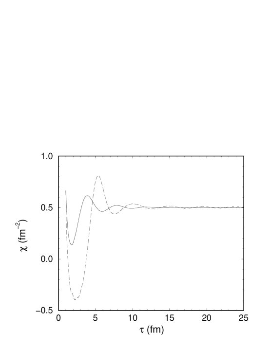
FIG. 1.: Proper time evolution of the $\chi$ field for the following initial conditions. Solid line: $\sigma(\tau_{0})=\sigma_{T}$, $\pi_{i}(\tau_{0})=0$, and $\dot{\sigma}(\tau_{0})=0$. Dashed line: $\sigma(\tau_{0})=\sigma_{T}$, $\pi_{i}(\tau_{0})=0$, and $\dot{\sigma}(\tau_{0})=-1$

FIG. 2.: Proper time evolution of the energy density and pressure for the initial conditions $\sigma(\tau_{0})=\sigma_{T}$, $\pi_{i}(\tau_{0})=0$, and $\dot{\sigma}(\tau_{0})=0$.

FIG. 3.: Proper time evolution of the energy density and pressure for the initial conditions $\sigma(\tau_{0})=\sigma_{T}$, $\pi_{i}(\tau_{0})=0$, and $\dot{\sigma}(\tau_{0})=-1$.

Figure 4 shows the conservation of the energy-momentum tensor. Notice that it is not conserved for short proper times. Because of the presence of the Landau pole it is not possible to take the physical cutoff $\Lambda$ very large (we use 800 MeV). Due to this rather small cutoff, the occupation number $n_{s_{m}}$ is not actually zero, which it was assumed to be for the derivation of the energy-momentum conservation [see the discussion after Eq. (91)]. As soon as the cutoff $s_{m}$ becomes large enough, then the occupation number goes to zero and the energy-momentum tensor is conserved. Figure 5 shows the energy-momentum tensor conservation for initial conditions with an instability. We see a qualitatively similar behavior, regardless of initial conditions.

FIG. 4.: Energy-momentum tensor conservation, for the initial conditions $\sigma(\tau_{0})=\sigma_{T}$, $\pi_{i}(\tau_{0})=0$, and $\dot{\sigma}(\tau_{0})=0$.

FIG. 5.: Energy-momentum tensor conservation, for the initial conditions $\sigma(\tau_{0})=\sigma_{T}$, $\pi_{i}(\tau_{0})=0$, and $\dot{\sigma}(\tau_{0})=-1$.

V Conclusions

We have shown how to regularize and renormalize the energy-momentum tensor for a spherically symmetric model with a time-dependent comoving momentum cutoff which breaks covariance. We computed the finite energy density and pressure, and numerically examined the equation of state and proved energy conservation for this system. We found that the energy density and pressure both decrease quickly, which is expected for a rapidly cooling system. An interesting feature of the expansion is that when the effective mass squared is negative, the pressure is also negative. A negative pressure implies cavitation, which could mean the formation of domains, i.e. DCCs.

A Christoffel symbols

The only non-vanishing Christoffel symbols for the metric

$$g_{\mu\nu}=C(u)\;{\rm diag}\;(1,-1,-\sinh^{2}\eta,-\sinh^{2}\eta\sin^{2}\theta)\>,$$ (A1)

with

$$C(u) = a^{2}(\tau)=\tau^{2}={\rm e}^{2u}/m^{2}\>,$$ (A2)

are

$$\begin{array}[]{rclrcl}\Gamma^{u}_{\eta\eta}&=&1\>,&\Gamma^{u}_{\theta\theta}&=&\sinh^{2}\eta\>,\\ \Gamma^{u}_{\varphi\varphi}&=&\sinh^{2}\eta\sin^{2}\theta\>,&\Gamma^{\eta}_{\theta\theta}&=&-\sinh\eta\cosh\eta\>,\\ \Gamma^{\eta}_{\varphi\varphi}&=&-\sinh\eta\cosh\eta\sin^{2}\theta\>,&\Gamma^{\theta}_{\varphi\varphi}&=&-\sin\theta\cos\theta\>,\end{array}$$

$$\begin{array}[]{rcccccccl}\Gamma^{u}_{uu}&=&\Gamma^{\eta}_{\eta u}&=&\Gamma^{\theta}_{\theta u}&=&\Gamma^{\varphi}_{\varphi u}&=&1\>,\end{array}$$

$$\begin{array}[]{rcccl}\Gamma^{\theta}_{\theta\eta}&=&\Gamma^{\varphi}_{\varphi\eta}&=&\coth\eta\>,\end{array}$$

$$\begin{array}[]{rcl}\Gamma^{\varphi}_{\varphi\theta}&=&\cot\theta\>.\end{array}$$

The Christoffel symbols are used to derive the conservation law for the energy-momentum tensor.

B Energy-momentum Tensor for a Perfect Fluid

For a perfect fluid we can write the energy-momentum tensor as follows

$$T_{\mu\nu}=-p\;g_{\mu\nu}+(\epsilon+p)\;u_{\mu}u_{\nu}\>,$$ (B1)

where $u_{\mu}$ are the components of the velocity vector of the fluid, such that it is normalized, i.e. $g^{\mu\nu}u_{\mu}u_{\nu}=1$, which corresponds to a timelike vector field. In the reference frame where the fluid is at rest we can write

$$u_{\mu}=(u_{u},u_{\eta},u_{\theta},u_{\varphi})=(u_{u},\vec{0})\>,$$ (B2)

and the normalization condition simply implies that $g_{uu}=u_{u}u_{u}=C(u)$. It is then straightforward to obtain the components of the energy-momentum tensor in this coordinate system

$$T_{uu} = g_{uu}\;\epsilon=C(u)\;\epsilon,$$ (B3)

$$T_{\eta\eta} = -g_{\eta\eta}\;p=C(u)\;p,$$ (B4)

$$T_{\theta\theta} = -g_{\theta\theta}\;p=C(u)\;p\sinh^{2}\eta,$$ (B5)

$$T_{\varphi\varphi} = -g_{\varphi\varphi}\;p=C(u)\;p\sinh^{2}\eta\sin^{2}\theta\>.$$ (B6)

Then we can write

$$\langle\,T_{\mu\nu}\,\rangle\equiv C(u){\rm diag}\,(\,\epsilon,\,p,\,p\,\sinh^{2}\eta,\,p\,\sinh^{2}\eta\sin^{2}\theta\,)\>.$$ (B7)

C Regularization by Covariant Geodesic Point-Splitting

The regularization scheme (introducing a physical momentum cutoff $\Lambda$) used to render the mode integrals finite in the energy density and isotropic pressure is not a covariant method. Since we must obtain covariant results (we want to obtain $\langle T_{\mu\nu}\rangle_{\rm renormalized}$), we have to proceed with care, in order to perform the physical subtractions that will yield the physical finite energy density and pressure. We shall make use of the results obtained by Christensen [4], in order to analyze the non-covariant structure on the divergences in $\epsilon_{0}$ and $p_{0}$, since we know that covariant point-splitting in a spatial direction is equivalent to regularization by introducing a momentum cutoff.

Christensen [4] obtained:

$$\langle T_{\mu\nu}\rangle_{quartic} = {\lim}_{x^{\prime}\rightarrow x}\frac{1}{2\pi^{2}}\frac{1}{{(\sigma^{\lambda}\sigma_{\lambda})}^{2}}\left(g_{\mu\nu}-\frac{4\sigma_{\mu}\sigma_{\nu}}{{(\sigma^{\lambda}\sigma_{\lambda})}}\right),$$ (C1)

$$\langle T_{\mu\nu}\rangle_{quadratic} = -{\lim}_{x^{\prime}\rightarrow x}\frac{1}{4\pi^{2}}\frac{1}{{(\sigma^{\lambda}\sigma_{\lambda})}}\frac{\chi}{2}\left(g_{\mu\nu}-\frac{2\sigma_{\mu}\sigma_{\nu}}{{(\sigma^{\lambda}\sigma_{\lambda})}}\right),$$ (C2)

$$\langle T_{\mu\nu}\rangle_{logarithmic} = -{\lim}_{x^{\prime}\rightarrow x}\frac{1}{4\pi^{2}}\frac{\chi^{4}}{8}g_{\mu\nu}\left(\gamma+\frac{1}{2}\ln\mid\frac{\chi\sigma}{2}\mid\right)\>.$$ (C3)

If we choose $\sigma_{\mu}$ to be a spacelike vector such that

$$\sigma_{i}\sigma_{j}=\frac{1}{3}g_{ij}(\sigma^{\lambda}\sigma_{\lambda})\;\;\;\;{\rm and}\;\;\;\;\sigma_{u}=0\;\;\;\;{\rm with}\;\;\;\;i,j=\eta,\theta,\varphi\>,$$ (C4)

we can write

$$\langle T_{uu}\rangle_{quartic} = {\lim}_{x^{\prime}\rightarrow x}\frac{1}{2\pi^{2}}\frac{1}{{(\sigma^{\lambda}\sigma_{\lambda})}^{2}}\;C(u),$$ (C5)

$$\langle T_{\eta\eta}\rangle_{quartic} = {\lim}_{x^{\prime}\rightarrow x}\frac{1}{2\pi^{2}}\frac{1}{{(\sigma^{\lambda}\sigma_{\lambda})}^{2}}\;\frac{C(u)}{3},$$ (C6)

$$\langle T_{uu}\rangle_{quadratic} = -{\lim}_{x^{\prime}\rightarrow x}\frac{1}{4\pi^{2}}\frac{1}{(\sigma^{\lambda}\sigma_{\lambda})}\;\frac{\chi}{2}\;C(u),$$ (C7)

$$\langle T_{\eta\eta}\rangle_{quadratic} = {\lim}_{x^{\prime}\rightarrow x}\frac{1}{4\pi^{2}}\frac{1}{{(\sigma^{\lambda}\sigma_{\lambda})}}\;\frac{\chi}{2}\;\frac{C(u)}{3},$$ (C8)

$$\langle T_{uu}\rangle_{logarithmic} = -{\lim}_{x^{\prime}\rightarrow x}\frac{1}{4\pi^{2}}\;\frac{\chi^{4}}{8}\;C(u)\left(\gamma+\frac{1}{2}\ln\mid\frac{\chi\sigma}{2}\mid\right),$$ (C9)

$$\langle T_{\eta\eta}\rangle_{logarithmic} = {\lim}_{x^{\prime}\rightarrow x}\frac{1}{4\pi^{2}}\;\frac{\chi^{4}}{8}\;C(u)\left(\gamma+\frac{1}{2}\ln\mid\frac{\chi\sigma}{2}\mid\right)\>.$$ (C10)

¿From Appendix B we know that $T_{uu}=C(u)\epsilon$ and that $T_{\eta\eta}=C(u)p$ and from the previous equations (C10) we can make the following identifications:

$$\epsilon_{quartic} = {\lim}_{x^{\prime}\rightarrow x}\frac{1}{2\pi^{2}}\frac{1}{{(\sigma^{\lambda}\sigma_{\lambda})}^{2}},$$ (C11)

$$p_{quartic} = {\lim}_{x^{\prime}\rightarrow x}\frac{1}{2\pi^{2}}\frac{1}{{(\sigma^{\lambda}\sigma_{\lambda})}^{2}}\;\frac{1}{3},$$ (C12)

$$\epsilon_{quadratic} = -{\lim}_{x^{\prime}\rightarrow x}\frac{1}{4\pi^{2}}\frac{1}{{(\sigma^{\lambda}\sigma_{\lambda})}}\;\frac{\chi}{2},$$ (C13)

$$p_{quadratic} = {\lim}_{x^{\prime}\rightarrow x}\frac{1}{4\pi^{2}}\frac{1}{{(\sigma^{\lambda}\sigma_{\lambda})}}\;\frac{\chi}{2}\;\frac{1}{3},$$ (C14)

$$\epsilon_{logarithmic} = -{\lim}_{x^{\prime}\rightarrow x}\frac{1}{4\pi^{2}}\;\frac{\chi^{4}}{8}\left(\gamma+\frac{1}{2}\ln\mid\frac{\chi\sigma}{2}\mid\right),$$ (C15)

$$p_{logarithmic} = {\lim}_{x^{\prime}\rightarrow x}\frac{1}{4\pi^{2}}\;\frac{\chi^{4}}{8}\left(\gamma+\frac{1}{2}\ln\mid\frac{\chi\sigma}{2}\mid\right)\>.$$ (C16)

Thus it follows

$$\epsilon_{quadratic} = 3\;p_{quadratic},$$ (C17)

$$\epsilon_{quartic} = -3\;p_{quartic},$$ (C18)

$$\epsilon_{logarithmic} = -\;p_{logarithmic}\>.$$ (C19)

We can now compare these general results for spatial point-splitting with Eqs. (70) and (73) by making use of the natural identification $\sigma^{\lambda}\sigma_{\lambda}\propto\Lambda^{-2}$. It is easy to see that the quartic, quadratic and logarithmic terms of these expressions fulfill the requirements of Eq. (C19), as we wanted to show.

REFERENCES

• [1] K. Rajagopal and F. Wilczek, Nucl. Phys. B399, 395 (1993);
S. Gavin, A. Gocksch and R.D. Pisarski, Phys. Rev. Lett.72, 2143 (1994);
S. Gavin and B. Müller, Phys. Lett. B 329, 486 (1994);
S. Gavin, in Relativistic Aspects of Nuclear Physics, Proceedings of the International Workshop, Rio de Janeiro, Brazil, 1993, edited by K. Chung et. al (World Scientific, Singapore, 1995), Report No. hep-ph/9407368 (unpublished);
D. Boyanovsky, H.J. de Vega, and R. Holman, Phys. Rev. D51, 734 (1995);
J.-P. Blaizot and A. Krzywicki, Phys. Rev. D46, 246 (1992); Phys. Rev. D50, 442 (1994).
• [2] M. A. Lampert, J.F. Dawson, and F. Cooper, Phys. Rev. D54, 2213 (1996), and references therein.
• [3] F. Cooper, Y. Kluger, E. Mottola, and J.P. Paz, Phys. Rev. D51, 2377 (1995).
• [4] S. M. Christensen, Phys. Rev. D17, 946 (1978).
• [5] F. Cooper, G. Frye, and E. Schonberg, Phys. Rev. D11, 192 (1975).
• [6] J. Schwinger, J. Math. Phys. 2, 407 (1961);
P. M. Bakshi and K. T. Mahanthappa, J. Math. Phys. 4, 1 (1963); 4, 12 (1963);
L. V. Keldysh, Zh. Eksp. Teo. Fiz. 47, 1515 (1964) [Sov. Phys. JETP 20, 1018 (1965)];
G. Zhou, Z. Su, B. Hao and L. Yu, Phys. Rep. 118, 1 (1985);
F. Cooper, S. Habib, Y. Kluger, E. Mottola, J.P. Paz and Paul Anderson, Phys. Rev. D50, 2848 (1994).
• [7] L. Parker and S. A. Fulling, Phys. Rev. D9, 341 (1974).
• [8] N.D. Birrell and P.C.W. Davies, Quantum Fields in Curved Space, (Cambridge University Press, 1982), p. 122.
• [9] C. G. Callan, S. Coleman, and R. Jackiw, Ann. Phys. (NY) 59, 42 (1970).
• [10] T. S. Bunch, J. Phys. A: Gen. Phys. 13, 1297 (1980).
• [11] D. J. Toms, Phys. Rev. D26, 2713 (1982).
• [12] C. T. Hill and D. S. Salopek, Ann. Phys. (NY) 213, 21 (1992).
• [13] F. Cooper, S. Habib, Y. Kluger, and E. Mottola, Phys. Rev. D55, 6471 (1997).