Abstract

The electromagnetic form factors of hadrons at large momentum transfer have been the subject of intense theoretical and experimental scrutiny over the past two decades, yet there is still not a universally-accepted framework for their description. This review is a synopsis of their current status at large momentum transfer. The basic theoretical approaches to form factors at large momentum transfer are developed, emphasizing the valence quark and Feynman (soft) pictures. The discussion includes the relation of these descriptions to the parton model, as well as the roles of factorization, evolution, Sudakov resummation and QCD sum rules. This is followed by a discussion of the experimental status of pion and nucleon elastic form factors and resonance production amplitudes in the light of recent data, highlighting the successes and shortcomings of various theoretical proposals.

 

1 Introduction

1.1 Hadronic Form Factors

Exclusive electromagnetic form factors are a source of information about the internal structure of hadrons. The coupling of an elementary particle to the photon is determined by only a few dimensionless parameters, for example its total charge and magnetic moment. For a composite particle, however, these constant coefficients are replaced by momentum-dependent functions, the form factors, which reflect the distribution of charge and current, and hence the internal structure of the particle. A familiar analysis in nonrelativistic quantum mechanics relates the electromagnetic form factor directly to the Fourier transform of the the charge density. Relativistic behavior also depends very much on the nature of the hadronic state.

High momentum transfer suggests high resolution, so hard elastic scattering is a natural way to study the detailed internal structure of hadrons. Experiments in elastic electron-proton scattering showed long ago the famous dipole behavior of the nucleon electromagnetic form factors in terms of momentum transfer $Q$, $1/(1+Q^{2}/M^{2})^{2}$, with $M\sim 0.71$ GeV² [1].

Since then, many subsequent experiments studied this and related reactions. Their influence on our understanding of the strong interactions themselves, however, has been somewhat overshadowed by that of the high energy inclusive reactions. The discovery of approximate scaling in deeply inelastic scattering, and its explanation in terms of the parton model, opened a more direct and efficient avenue to study the quarks themselves, since inclusive rates decay much more slowly with momentum transfer. Nevertheless, form factors at large momentum transfer remain an important window to quark binding in hadrons.

In this review, we will concentrate on electromagnetic form factors and resonance production amplitudes, at large momentum transfer, in the light of perturbative quantum chromodynamics (QCD). QCD itself has enjoyed so many successes, and explains so many and varied experimental results, that it is universally recognized as “the” theory of the strong interactions. Yet, the single most basic fact of the theory, the binding and confinement of the elementary degrees of freedom, the quarks and gluons, into hadrons, is still not described in detail. Because of the property of asymptotic freedom at short distances, perturbative methods must be relevant in some degree to elastic scattering at large momentum transfer. Because the binding of hadrons is a long-distance effect, nonperturbative effects must play a crucial role as well. The description of electromagnetic form factors requires the consistent analysis of both length scales in a single process. This, and the light that will be shed on hadronic structure by a truly successful treatment of this problem makes the study of form factors attractive. We note that electromagnetic form factors are part of the large class of exclusive hadronic amplitudes, which also describe, for example, both proton-proton elastic scattering and the exclusive decays of heavy mesons. Although many of the methods developed below have wide applications in this larger class, we decided to restrict our discussion to form factors, in the hope of improving its focus.

In the remainder of this section, we discuss what we can learn from reasoning based on the parton model. Here, and in most of the following, we assume very high momentum transfer, so high that parton masses may for the most part be neglected. We use parton model insights to identify quark counting rules, and as an inspiration for factorization of long- and short-distance effects in exclusive processes in terms of wave functions. In this section, we give primarily intuitive arguments, and concentrate for simplicity on the pion. In Sec. 2, we discuss some of the central results of the QCD treatment of form factors, including the evolution of wave functions, the behavior of the asymptotic pion form factor, and QCD sum rules for moments of wave functions. These topics are somewhat more mathematical, but we have attempted to motivate technical arguments with physical intuition. We close this section with a brief summary of results relevant to baryons, especially helicity conservation, the derivation of form factors directly from QCD sum rules, and a few phenomenological models for moderate-$Q^{2}$ behavior. We go on to review the central experimental results for pion, nucleon and resonance production form factors, to assess the successes and failures of QCD treatments of elastic scattering, and to explain the controversies that have enlivened this active field of inquiry. To anticipate, we will see that the current state of the data is not adequate to resolve the primary theoretical controversies.

1.2 Partons and Factorization

1.2.1 Partons. The perturbative treatment of hard exclusive processes assumes a partonic description of the participating hadrons. The general discussion is closely related to the parton model of inclusive processes [2], such as deep-inelastic scattering. The celebrated premise of the parton model, justified and systematically extended in QCD, is that inclusive processes are determined by the distributions $f_{i/h}(x)$, which are the probabilities for pointlike, constituent partons $i$ to carry fraction $x$ of the momentum of hadron $h$, summed over all other partonic degrees of freedom. An exclusive form factor, on the other hand, reflects the coherent scattering of a hadron by an electroweak current. Even at large momentum transfer, it may depend on states of definite partonic content. In fact, at high enough energies, exclusive amplitudes are dominated by hadronic states with “valence” quark content, ${\bar{\rm q}}{\rm q}$ for mesons and qqq for baryons. This is despite the fact that, in its own rest frame, each hadron is a complicated, ever-shifting superposition of partonic states. Let us discuss first how such a partonic picture of hard exclusive scattering emerges.

At sufficiently high momentum transfers in either hadron-lepton or hadron-hadron scattering, the relative velocities of all participating particles are nearly lightlike. Under this condition, the quantum processes that bind the constituents of a hadron are highly time-dilated in the rest frames of the remaining particles, both incoming and outgoing. Correspondingly, time dilation lengthens the lifetime of these states, and “freezes” the partonic content of this hadron as “seen” by the other particles. Also, as relative velocities approach the speed of light, the time during which the hadrons remain in contact, and during which momentum can be transferred, decreases. In fact, we can always find a frame in which any pair of particles are in contact for a time that decreases like $1/\gamma_{\rm rel}=\left(1-v_{\rm rel}^{2}/c^{2}\right)^{1/2}$. Under these conditions, we expect a lack of quantum interference between long-distance, hadronic binding and short-distance momentum transfer. This incoherence between soft and hard physics implies that we may consider each hadron to consist of a definite partonic state during the entire collision process. This picture is illustrated for electron-pion scattering in Fig. 1a, in which long-time dynamics, described by a distribution of valence quarks $\phi_{\rm in}$, produces a “valence” quark-antiquark state. The distribution $\phi$ is often referred to as a “wave function”. The partons of this state in turn exchange momentum with an electron in a short-distance process $T$. At a later time, they reform a pion, through wave function $\phi_{\rm out}$.

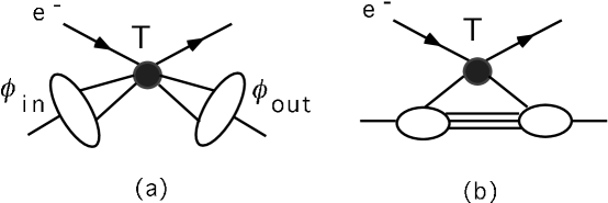
Figure 1: Electron-pion elastic scattering. a) Valence PQCD picture. b) Feynman mechanism.

1.2.2 Factorization. We summarize the above considerations for an arbitrary exclusive amplitude $M$ by a schematic expression in which short-distance momentum transfer is factorized from the long-distance hadronic binding,

$$M(p_{i}\cdot p_{j})=\prod_{j}\phi_{{\rm out},j}(n_{j})\otimes T(n_{j},n_{i})\otimes\prod_{i}\phi_{{\rm in},i}(n_{i})\,.$$ (1)

Here, the labels $i$ and $j$ refer to hadrons in the incoming and outgoing states, respectively. $\phi(n)$ is the wave function that describes the amplitude for a pion to be found in partonic state $n$, and $T(n_{j},n_{i})$ is a perturbative function that describes the hard scattering between the partons (and leptons). The symbol $\otimes$ indicates a convolution, that is, a sum or integral over the parton degrees of freedom that correspond to states $n_{i}$ and $n_{j}$.

A factorized expression like Eq. (1) has two fundamental properties. First, the nonperturbative wave functions are universal within a class of exclusive amplitudes. This connects otherwise disparate processes, such as the pion electromagnetic form factor and pion-pion elastic scattering [3]. Second, the factorization of long- from short-distance dynamics implies consistency conditions that enable us to compute the amplitude’s dependence on the momentum transfer. These are usually referred to as “evolution” equations, examples of which we shall discuss below. The details of the convolution $\otimes$, and the derivations of evolution equations, depend on the process in question, but one example will suffice to motivate Eq. (1) and to illustrate the range of possibilities, the electromagnetic form factor of the charged pion. We will review the classic perturbative QCD analysis of this form factor [4, 5, 6], and also introduce a treatment of its “Sudakov” effects [7, 8], whose importance will become clear below.

1.2.3 Valence PQCD and the Feynman Mechanism. The convolutions $\otimes$ in Eq. (1) in principle include sums over states with arbitrary numbers of partons. As indicated above, however, at very large momentum transfer, the valence state, with the fewest partons, dominates. We shall refer below to its contribution as “valence perturbative QCD” (valence PQCD). This is a somewhat unconventional usage; indeed, what we call valence PQCD is more commonly referred to simply as “PQCD”. But this approximation does not exhaust the use of perturbative methods in form factors at large momentum transfer, and to call it simply “PQCD” is a little misleading.

There are, of course, many contributions from states with more than the valence partons. For the most part, they are expected to decay rapidly with increasing momentum transfer, relative to the valence states. There is an exception, however, corresponding to states in which one parton carries nearly all of the hadron’s momentum, while all other partons are soft. It is plausible that such a state could contribute to elastic scattering, because all of its partons except for one have long wavelengths. They may then overlap strongly with wave functions moving in any direction. When the single, hard parton scatters elastically, the soft partons from an incoming hadron may combine with the outgoing hard parton to form an outgoing hadron. This is illustrated for the pion electromagnetic form factor in Fig. 1b. It is known as the “soft” or “Feynman” mechanism for elastic scattering. Nevertheless, the Feynman mechanism contains a hard scattering, which may, in principle, be factored from the interactions of soft partons, and treated with the methods of PQCD. For instance, in [9, 10] it was analyzed for pion and nucleon form factors. This PQCD investigation, unfortunately, has not yet been developed extensively in the literature, and although it seems clear that the soft mechanism does not contribute at asymptotically high momentum transfer, at what scale it becomes negligible is not well understood. We shall come back to the role of the soft mechanism often below, however, because its contribution may be studied directly in the valence state, using Sudakov resummation, and in QCD sum rules, and, indirectly, in models of nonperturbative hadronic structure.

1.2.4 The Pion Form Factor and Quark Counting. The electromagnetic form factor of a pion is specified by

$$\left(p_{2}+p_{1}\right)_{\mu}F_{\pi}(Q^{2})=\langle\pi(p_{2})|J_{\mu}(0)|\pi(p_{1})\rangle\,,$$ (2)

where $J_{\mu}=\sum_{f}e_{f}{\bar{q}}_{f}\gamma_{\mu}q_{f}$ is the electromagnetic current, expressed in terms of quark fields $q_{f}$ of flavor $f$ and electromagnetic charges $e_{f}$. We neglect particle masses, and examine this process in a “brick-wall” frame, in which $p_{1}$ is in the plus 3 direction, and recoils as $p_{2}$ in the minus 3 direction under the influence of the electromagnetic current $J$. Such a momentum configuration is most naturally described in terms of light-cone variables, which for any vector $v^{\mu}$ are $v^{\pm}=2^{-1/2}(v^{0}\pm v^{3})$. In these terms we have

$$p_{1}^{+}={Q/\sqrt{2}},\ p_{1}^{-}=0,\quad\quad p_{2}^{-}={Q/\sqrt{2}},\ p_{2}^{+}=0\,.$$ (3)

The overall momentum transfer is $(p_{2}-p_{1})^{2}=-2p_{1}^{+}p_{2}^{-}=-Q^{2}$.

The valence PQCD portrait of this process is shown in Fig. 2. Fig. 2a represents the pion in its valence state, consisting of a quark and an antiquark. The variable $x$ denotes the fraction of the pion’s momentum carried by the quark and $1-x$ by the antiquark. In the chosen frame, we expect the pion to be Lorentz contracted in the direction of motion, as shown, so that the pair is localized in this direction. On the other hand, we expect the partons in any virtual state to be more-or-less randomly distributed in the transverse extent of the pion’s wave function, since the boost from the rest frame to the frame under consideration leaves transverse positions unchanged. This will have important consequences below. Similarly, the off-shellness, and the transverse momenta of the pair in Fig. 2 are boost-invariant, and we take these quantities to be fixed, and negligible compared to both $xp_{1}$ and $(1-x)p_{1}$. Correspondingly, the transverse components of their velocities vanish as $Q\rightarrow\infty$, and we neglect them as well. It is necessary that $1>x>0$, so that both partons travel in the same direction as the hadron that they represent. Fig. 2a also shows an incoming, off-shell photon, carrying momentum $q$.

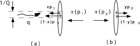
Figure 2: Pion electromagnetic form factor in valence PQCD.

Fig. 2b shows the state of the system after the action of the current that absorbs the photon, in which the pair moves in the opposite direction. Eventually, the pair will fill out the full spatial extent of the pion, which is again Lorentz contracted. To form the pion, however, their momenta must be parallel, and each must carry a positive fraction of $p_{2}$, as shown.

An alternative picture relies on the “infinite momentum frame” (IMF), in which all participating particles move in the same direction, with energies $E_{i}\gg Q$. In this frame, all momentum transfers are transverse. Its main attraction lies in the conjecture that quantization formulated in an IMF simplifies the treatment of confinement in QCD [11].

In the process depicted in Fig. 2, the quark undergoes a momentum transfer $xyQ^{2}$, and the antiquark $(1-x)(1-y)Q^{2}$, with $x$ ($y$) the fractional momentum of the quark in the incoming (outgoing) pion. This must take place during the time that the wave functions of the incoming and outgoing pions overlap, that is, on a time scale that vanishes as $1/Q$. The uncertainty principle requires that both members of the pair must be localized within $1/Q$ of each other and of the action of the current, as indicated in Fig. 2a. This restriction shows, first of all, that not all details of the valence state wave function are relevant to exclusive scattering. We do not need the full two-particle state; we only need the probability for the members of the pair to be within a transverse distance of $1/Q$ of each other. We shall assume that this probability is simply a function of $x$ times the geometrical factor $1/Q^{2}$. This “scaling” of the wave function in $x$ is not exact in QCD; we will compute corrections to it when we discuss evolution below in Sec. 2.2.

Along with our assumption of incoherence, scaling enables us to estimate the $Q$-dependence of the form factor. For, if long- and short-distance processes are incoherent, the cross section for elastic scattering of a pion is essentially the product of the cross section for the elastic scattering of a point-like scalar particle, times the probability for internal processes to produce a virtual state in which both partons in the valence state are within $1/Q$ of each other in transverse distance. Thus, we have

$$\sigma_{{\rm el},\pi}\ \sim\ \sigma_{\rm el,\ point}\times F_{\pi}^{2}(Q^{2})\ \sim\ \sigma_{\rm el,\ point}\times(1/Q^{2})^{2}$$ (4)

so that

$$F_{\pi}(Q)\sim(1/Q^{2})\,.$$ (5)

Results of this sort, based on incoherence, scaling and geometrical estimates, are known as “quark counting” [12, 13]. Quark counting rules give for an arbitrary exclusive process involving $n_{h}$ hadrons,

$$\sigma(Q^{2})_{\rm had}=\sigma(Q^{2})_{\rm point}(Q^{2})^{-n_{q}+n_{h}}f\,,$$ (6)

where $n_{q}$ is the total number of quarks and antiquarks taking part in the process, and $f$ depends on dimensionless variables.

¿From Eq. (6), we see that interactions involving more than the minimum number of partons – say, a gluon in addition to the pair – are suppressed by a power of $Q$, because as $Q$ grows, the likelyhood of finding more than the minimum number of particles within $1/Q$ of each other falls as $Q^{-2}$ for each additional particle.

We note, however, that in the limits $x,y\rightarrow 0,1$, our process describes the elastic scattering of an on-shell quark (antiquark) with nearly all of the pion’s momentum. The remaining, soft antiquark (quark) has long wavelength, which overlaps with both the incoming and outgoing wave functions. This is the intersection of valence PQCD with the Feynman mechanism.

In the next section, we shall turn to the field-theoretic treatment of the pion’s form factor, and shall see how these features of the parton model are realized within QCD.

2 Form Factors in QCD

2.1 The Factorized Pion Form Factor

2.1.1 Convolution in Fractional Momenta. We are now ready to turn to the pion form factor in valence PQCD [4, 5, 6]. The parton model discussion of the previous section suggests that the pion form factor can be written, following Eq. (1), as a sum over wave functions involving only quark momentum fraction. We denote these as $x$ and $y$ for the incoming and outgoing pions, respectively. We then have the following representation for the form factor,

$$F_{\pi}(Q^{2})=\int_{0}^{1}dx\;dy\;\phi_{\pi}(y,\mu^{2})\;T(y,x,Q^{2},\mu^{2})\;\phi_{\pi}(x,\mu^{2})\,.$$ (7)

Here, $\phi_{\pi}(x,\mu^{2})$ is the valence-state wave function describing a quark with fraction $x$ of the pion’s momentum. $T(x,y,Q^{2},\mu^{2})$ describes the hard scattering of partons. It is a perturbative expansion in the strong coupling at scale $\mu^{2}$ ($\alpha_{s}(\mu^{2})$), and is free of infrared divergences order-by-order in perturbation theory. At lowest order, it is given by the diagrams shown in Fig. 3a. Since the incoming and outgoing pairs are each at a tiny transverse separation, orbital angular momenta are negligible, and partonic helicities must sum to zero. The pairs of incoming and outgoing external lines in the diagrams are thus projected onto Dirac matrices that represent these helicity-zero pairs. [6] At the same time, because masses are neglected, helicities are conserved in perturbation theory, and hence in the hard scattering, to all orders. This has important consequences for hadrons with spin. An exercise in dimensional counting shows that $T$ has dimensions (mass)^-2, and hence scales as $1/Q^{2}$. Its explicit lowest-order form is

$$T_{H}=16\pi C_{F}\alpha_{s}(\mu^{2})\left[{2\over 3}{1\over xyQ^{2}}+{1\over 3}{1\over(1-x)(1-y)Q^{2}}\right]\,,$$ (8)

where $C_{F}=(N^{2}-1)/2N=4/3$ in QCD.

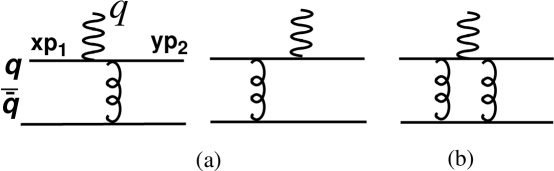
Figure 3: Graphical contributions to $T$: (a) Lowest order; (b) Typical one-loop correction.

In perturbation theory, it is possible to show that the valence PQCD result Eq. (7) is a theorem, which describes the behavior of $F_{\pi}(Q^{2})$ at large $Q^{2}$ to all orders in $\alpha_{s}$. Corrections are suppressed by powers of $Q^{2}$, including those due to the Feynman (soft) mechanism described above [5, 6, 10]. Helicity conservation in $T$ is also valid up to similar corrections. Space does not allow a discussion here of technical aspects of this proof or of the calculation of $T$ beyond lowest order. The basic technique is already illustrated by a typical one-loop correction, Fig. 3b. (For the pion form factor, the full one-loop calculation has been performed explicitly [14, 15]. We keep only those contributions to $T$ from Fig. 3b where all quark and gluon lines are off-shell by at least the renormalization scale, $\mu^{2}$. $T$ then depends on only two momentum scales, $Q$ and $\mu$. Alternately, we can think of $\mu^{2}$ as the minimum transverse momentum carried by lines in $T$. Suppose, now, that we choose $\mu=Q$. By the uncertainty principle, this corresponds to including in $T$ only lines that are within $1/Q$ of each other in transverse distance, as we anticipated in our discussion of Fig. 2 above. By choosing $Q=\mu$ we get the extra benefit of expanding $T$ in terms of the small parameter $\alpha_{s}(Q^{2})$. Thus, $\mu=Q$ will be our default choice of scale below, although other choices may sometimes offer special advantages.

2.1.2 Transverse Degrees of Freedom in $F_{\pi}$. Our next exercise in factorization is to return to Eq. (7), taking into account transverse degrees of freedom. Remaining in the valence picture, we recall that the pair in the incoming and outgoing pions are not literally at a point, but are separated by transverse vectors $b_{i}$ when they undergo the hard scattering, where $i=1\,(2)$ for the incoming (outgoing) pion. Again, $Q^{2}=(p_{2}-p_{1})^{2}$. The wave functions in Eq. (1), which we now denote $\cal P$, are characterized by both fractional momenta and transverse separation, and the form factor is reexpressed as a convolution in both [8],

$$F_{\pi}(Q^{2}) = \int_{0}^{1}dxdy\;\int{d^{2}b_{1}\over(2\pi)^{2}}{d^{2}b_{2}\over(2\pi)^{2}}\;{\cal P}(y,b_{2},p_{2},\mu)$$ (9)

$$\hbox{\hskip 42.67912pt}\times\;T(y,x,p_{i},b,\mu)\;{\cal P}(x,b_{1},p_{1},\mu)\,,$$ (10)

where $T$ is a new hard-scattering function. Beause we integrate over the variables $b_{i}$ conjugate to transverse momenta, $\mu$ does not play the role of a “transverse momentum cutoff”, as in Eq. (7), but is simply the renormalization scale. On the other hand, the wave functions $\cal P$ depend upon the momenta $p_{i}$ and they, along with $T$, are not individually Lorentz invariant. The requirement of Lorentz invariance in the complete amplitude $F_{\pi}$ will lead to evolution equations below. We emphasize that, summed to all orders, Eq. (10) is equivalent to Eq. (7) at leading power in $Q^{2}$. Depending on the details of $\cal P$, however, it differs from Eq. (7) in nonleading powers of $Q^{2}$ in general.

We next explore the relation between the two factorization procedures a little further. Intuitively, we expect that the wave function $\cal P$ near $b=0$, that is at small separation for the pair, is related to the distribution amplitude $\phi_{\pi}$. Specifically, it is not difficult to show that [7]

$${\cal P}(x,b=1/\mu,p_{i},\mu)\ \sim\ \phi(x,\mu^{2})\,,$$ (11)

up to corrections that are suppressed by the strong coupling evaluated at the factorization scale $\mu$. The Lorentz noninvariance of the $\cal P$ disappears in this limit.

Let us now compare Eq. (10) to the classic expression, Eq. (7). If $Q^{2}$ is large enough, we expect, according to our discussion above, that $T$ in Eq. (10) is concentrated near $b\sim 1/Q$, so that by Eq. (11) $\cal P$ may be replaced by $\phi_{\pi}$. In this limit, the two expressions are equivalent. A closer look at $T$ in Eq. (7), however, shows that it actually corresponds to a localization in transverse space only at the scale $(xyQ^{2})^{-1}$. When $x$ or $y$ vanishes, the hard scattering “spreads out” in transverse space, and violates the original assumptions of the partonic discussion of Sec. 1.2.1 above, and the reaction is defined by the Feynman mechanism. Also note that if $b$ is large, the neglect of orbital contributions to helicity is no longer justified, even if helicity is conserved in the hard scattering [16, 17, 18]. The contribution of the “end-point regions” $x,y\rightarrow 0,1$ (the equivalent of the Feynman mechanism for ${\rm{\bar{q}}q}$ states) depends on the details of the wave functions $\phi$, but it poses a problem, unless $Q$ is very large [19, 20] We shall see shortly that the use of the modified factorization in Eq. (10) serves to stabilize the valence PQCD picture of scattering at somewhat lower $Q^{2}$ than in Eq. (7) [8]. To see how this comes about, we turn now to a discussion of evolution, as derived from the factorization formulas Eq. (7) and Eq. (10).

2.2 Evolution and Asymptotic Behavior

Eqs. (7) and (10) for the elastic form factor are both convolutions of functions that depend upon arbitrary choices: the renormalization scale $\mu$ in the former case, and the Lorentz frame in the latter. In fact, a great deal can be learned from these parameters, through their role in the factorization formulas. Among other things, it will allow us, in the following subsection, to give an explicit expression for the asymptotic behavior of $\phi_{\pi}$ and the form factor at high momentum transfer.

2.2.1 Evolution. Consider Eq. (7) for $F_{\pi}(Q^{2})$. The physical form factor, of course, cannot depend upon $\mu$:

$$\mu{d\over d\mu}F_{\pi}(Q^{2})=0\,.$$ (12)

Equivalently, in terms of the hard-scattering and wave functions,

$$0 = \int_{0}^{1}dxdy\bigg{[}{d\phi_{\pi}(y)\over d\mu}T\phi_{\pi}(x)+\phi_{\pi}(y){dT\over d\mu}\phi_{\pi}(x)$$ (13)

$$\hbox{\hskip 42.67912pt}+\ \phi_{\pi}(y)T{d\phi_{\pi}(x)\over d\mu}\;\bigg{]}\,.$$ (14)

This expression may be treated by separation-of-variable techniques. $d\phi_{\pi}(y,\mu^{2})/d\mu$, for instance, may depend upon the variables $y$ and $\mu^{2}$ only, the latter only through $\alpha_{s}(\mu^{2})$ (since there are no other dimensionless variables available.) In fact, its derivative with respect to $\mu^{2}$ must be perturbatively calculable, because changes in $\mu$ shift contributions from lines that are off-shell by order $\mu^{2}$ between $\phi_{\pi}$ and $T$. (See Sec. 2.1.1).) The most general form that satisfies these requirements is itself a convolution [6]:

$$\mu{d\phi(y,\mu^{2})\over d\mu}=\int_{0}^{1}dz\,V(y,z,\alpha_{s}(\mu^{2}))\phi_{\pi}(z,\mu^{2})\,.$$ (15)

The kernel $V$ is a distribution, rather than a simple function of $y$ and $z$, but its integral with any smooth function is finite. Given the convolution form Eq. (7) for the form factor, the evolution equation (15) holds to all orders in $\alpha_{s}(\mu^{2})$. Its explicit one-loop form is simply the coefficient of $\ln Q^{2}$ in the sum of one-loop corrections to the hard scattering, such as Fig. 3b. The kernel $V$ is known up to two loops [21]. We shall not exhibit its explicit form, but only note that, with the one-loop $V$, Eq. (15) may be solved explicitly. The most general solution is an expansion in Gegenbauer polynomials $C_{n}{}^{3/2}$ [6] [22],

$$\phi_{\pi}(x,\mu^{2})=x(1-x)\sum_{n\geq 0}a_{n}C_{n}^{3/2}(2x-1)\big{(}\ln{\mu^{2}\over\Lambda^{2}}\big{)}^{-\gamma_{n}/2\beta_{2}}\,,$$ (16)

with $\beta_{2}=(33-2n_{f})/12$ the one-loop coefficient of the QCD beta function, the $\gamma_{n}$ known anomalous dimensions and the $a_{n}$ arbitrary coefficients.

Space allows us to make only a few observations on this fascinating result: (i) The $a_{n}$ are linear combinations of matrix elements, identified in Sec. 2.3 below; (ii) $\gamma_{0}=0$. This is because the $n=0$ wave function, $\phi_{0}(z)=a_{0}z(1-z)$ gives zero when integrated with the one-loop kernel in Eq. (15). We shall refer to this “asymptotic” form of the pion wave function many times below; (iii) for $n>0$, all $\gamma_{n}>0$, which implies that as $\mu^{2}\to\infty$, all $x$-dependence in (16) that is not in the form of the asymptotic wave function decays, albeit only logarithmically.

2.2.2 Sudukov Resummation. Turning now to factorization in transverse space, we see that the factorization Eq. (10) suggests another evolution equation, this time in the momentum scale $Q$, which enters the wave functions through (non-invariant dependence on) the momentum vectors $p_{i}$. This equation will allow us to resum perturbative logarithms of the form $\ln(Qb)$, with $b$ the distance between the hard scatterings, an example of “Sudakov resummation”. The derivation of this equation is given in a related context in [7]. Here, we shall content ourselves with a physical explanation and the basic results. In brief, the effect of the resummation will be to suppress the nonperturbative contribution to $F_{\pi}$, and thus to extend valence PQCD to lower $Q^{2}$.

For large momentum transfer, the dynamics of elastic scattering strongly disfavors configurations in which $b$ is large. The physical reason for this result is that an isolated accelerated charge must radiate, by correspondence to classical gauge theory. As $b$ grows, the two charges associated with quark and antiquark become more isolated, and have correspondingly more tendency to radiate gluons. In elastic scattering, however, such radiation is forbidden by definition. Perturbatively, this manifests itself in the presence of double-logarithmic (“Sudakov”) corrections of the form $\alpha_{s}^{n}(\mu)\ln^{2n}(bQ)$. We therefore expect that the double logarithms at large $b$ will suppress configurations for which the charges are separated far enough to couple strongly to radiated gluons. Because the effect is essentially classical, it is necessary to sum to all orders (take the limit of large quantum numbers) to make this suppression manifest.

In this case, an evolution equation is derived from the independence of expressions like Eq. (10) of the choice of inertial frame. An infinitesimal Lorentz transformation changes the arguments of the $\cal P$’s and of $T$, but otherwise leaves the amplitude invariant. A full derivation (see [7]; the reasoning there is an application of a method first developed in Ref. [23]) requires more analysis of $b$ and $Q$ dependence in $T$ than we have room for here. The result is the following evolution equation, which takes the place of Eq. (15). Taking $p^{+}=Q$ in the center-of-mass frame, we have,

$$Q{\partial\over\partial Q}{\cal P}(x,b,p,\mu)=\left[K(b\mu)+G(x,Q/\mu)\right]{\cal P}(x,b,p,\mu)\,,$$ (17)

in which the functions $K$ and $G$ may be computed in perturbation theory. $K$ depends only on the “infrared” variable $b$, and $G$ on the “ultraviolet” variable $Q$.

The details of the solution to this equation is straightforward, and may be found in [7]. The result is striking:

$${\cal P}(x,b;p,\mu)={\rm e}^{-S(x,b,Q,\mu)}\bigg{(}\phi_{\pi}(x,1/b^{2})+{\cal O}\left(\alpha_{s}^{2}(1/b)\right)\bigg{)}\,,$$ (18)

where $\phi_{\pi}$ is the usual light-cone wave function for the pion, now evaluated at $\mu=1/b$. The Sudakov exponent $S$ strongly suppresses the wave function at large $b$, through the summation of double logarithms of $bQ$ per loop,

$$S=C_{F}\int_{1/b}^{xQ}{d\mu^{\prime}\over\mu^{\prime}}{\alpha_{s}(\mu^{\prime})\over\pi}\ln\left({xQ\over\mu}\right)+\ x\leftrightarrow 1-x+\dots\,,$$ (19)

where we have suppressed terms with fewer logarithms per loop. Note in particular that within the integral the perturbative coupling runs with the variable $\mu^{\prime}$, so that the Sudakov exponent $S$ diverges at $b=1/\Lambda_{\rm QCD}$. When $Q\gg\Lambda_{\rm QCD}$, the exponent is large, and the suppression great, whenever $b\gg 1/Q$, even for $b\ll 1/\Lambda_{\rm QCD}$. The quark-antiquark state with opposite helicties again dominates in this limit. The suppression of large-$b$ configurations has many applications to hadron-hadron reactions, and helps justify the concept of “transparency” in hadron-nucleus scattering [24].

2.2.3 The Asymptotic Form Factor. We are now ready to discuss one of the central results of the perturbative treatment, the asymptotic behavior of the pion electromagnetic form factor. We begin by recalling that the natural choice of scale in the factorized expression Eq. (7) is $Q=\mu$ (See Sec. 2.1.1). For $Q$ large enough, then, the wave function will be dominated by the $a_{0}$ term in its expansion (16), and $T$ will be well-approximated by its lowest-order contribution, Eq. (8). The $x$ and $y$ integrals in (7) are then simple, and the only remaining uncertainty is in a factor of $a_{0}^{2}$.

To fix $a_{0}$, we observe that the decay of the charged pion though the weak interactions may be treated by the same method of factorizing hard and soft degrees of freedom. In this case, the hard interaction is at a scale of the order of the W-mass, and the wave function of Eq. (16) is again dominated entirely by its $a_{0}$ coefficient. Then, defining the pion decay constant $f_{\pi}$ by (with $f_{\pi}\sim 93\;{\rm MeV}$)

$$\langle 0|{\bar{d}}(0)\gamma^{\mu}(1-\gamma_{5})u(0)|\pi(p)\rangle=-\sqrt{2}p^{\mu}f_{\pi}\,,$$ (20)

we may identify $a_{0}=\sqrt{3}f_{\pi}$ in Eq. (16). (More generally, we have $3f_{\pi}/\sqrt{N}$ with $N$ the number of colors). This result, along with properties of the anomalous dimensions ($\gamma_{n}>0$ for $n>0$), allows us to identify the large $\mu^{2}$ (or $Q^{2}$) behavior of the pion’s quark wave function:

$$\phi_{\pi}(x,\mu^{2})\rightarrow\sqrt{3}f_{\pi}x(1-x)\,.$$ (21)

This is generally referred to as the asymptotic wave function of the pion. We emphasize that it is model-independent.

Substituting Eq. (21) into Eq. (7), and using the lowest order hard-scattering function $T$ (Eq. (8)) with $\mu=Q$, we find an elegant expression for the pion form factor at high energy, which is valid up to corrections in $\alpha_{s}(Q)\sim 1/\ln(Q)$ [5, 6],

$$F_{\pi}(Q^{2})={12f_{\pi}^{2}\pi C_{F}\alpha_{s}(Q^{2})\over Q^{2}}\,.$$ (22)

2.2.4 Sudakov Resummation for $F_{\pi}$. With an eye to contributions for which the pair is widely separated, we may also use the Sudakov-resummed transverse wave function (18) in Eq. (10), to get

$$F_{\pi}(Q^{2}) = \int_{0}^{1}dxdy\;\int{d^{2}b\over(2\pi)^{2}}\;\phi_{\pi}(y,1/b^{2})\;{\rm e}^{-S(y,b,Q,\mu)}$$ (23)

$$\ \times\;T(y,x,Q,b,\mu)\;{\rm e}^{-S(x,b,Q,\mu)}\;\phi_{\pi}(x,1/b^{2})\,,$$ (24)

where we have simplified to a single transverse separation [8, 25]. The Sudakov exponential in this expressions factor suppresses contributions from $b\gg 1/Q$. The natural scale of the coupling in $T$ is $\mu\sim 1/b$, even in the end-point region. Perturbation theory thus remains self-consistent, by the dynamical suppression of the overlap region of valence PQCD and the soft mechanism. For moderate $Q^{2}$, however, $F_{\pi}$ still receives substantial contributions from relatively large $b<1/\Lambda_{\rm QCD}$. In this region, (24) should be thought of as a valence PQCD model for $F_{\pi}$. Form factors computed according to each of these procedures will be confronted with the data in Sec. 3 below.

2.3 Wave Functions and Nonperturbative Analysis

In the factorized picture of elastic scattering we treat hadrons as superpositions of states, each with definite numbers and positions (or momenta) of partons. Also, as we have seen, it is the states with the fewest partons - the “valence states” that dominate exclusive processes at sufficiently high $Q^{2}$ . Relativistic valence wave functions for valence states may be identified with matrix elements that connect single-particle states of definite hadron momentum $|h(p)\rangle$, with the hadronic vacuum $|0\rangle$ by the action of fields that absorb the relevant valence quanta. The analysis of these matrix elements can lead to valuable nonperturbative information, which supplements the purely perturbative results outlined above.

2.3.1 Matrix Elements. The light-cone wave function in position space for the valence state of a $\pi^{+}$ may be defined in terms of the matrix element of an up quark field $u$ with a conjugate down quark field,

$$\Psi(z\cdot p,z^{2})=\langle 0|\bar{d}(0)\;\gamma^{+}\gamma_{5}u(z)|\pi^{+}(p)\rangle\,,$$ (25)

where $p$ is taken in the plus direction. In the following, we shall generally neglect hadronic masses. We recall that $\gamma^{\pm}={1/\sqrt{2}}\left(\gamma^{0}\pm\gamma^{3}\right)$. So that $\Psi(z\cdot p,z^{2})$ may have a natural interpretation in terms of independent measurements of the up and antidown quark fields, we choose the separation between the two fields to be spacelike, $z^{2}<0$. The Dirac structure $\gamma^{+}\gamma_{5}$ projects out precisely the zero-helicity combinations of the quark and antiquark fields.

As defined, the wave function $\Psi$ of Eq. (25) is gauge-dependent. A common choice of gauge for the gluon field $A$ is $A^{+}=0$ for a pion moving in the plus direction. Alternately, we may connect the fields ${\bar{d}}(0)$ and $u(z)$ by a path-ordered exponential in the direction $z^{\mu}$, $P\exp\left[\int_{o}^{1}dtz^{\mu}A_{\mu}(zt)\right]$, with $A_{\mu}$ expressed as a matrix in the quark representation.

The momenta of the partons in the valence state may be fixed by taking Fourier transforms. For $\phi_{\pi}(x)$, we fix the fractional momentum of the quark to be $xp$ in the pion’s direction of motion, and integrate freely over all of its other components (and hence those of the antiquark) by setting $z^{+}=z_{T}=0$, and taking the transform of $\Psi$ with respect to $z^{-}$,

$$\phi_{\pi}(x,\mu^{2})=\int_{-\infty}^{\infty}{dz^{-}\over 2\pi}\;{\rm e}^{iz^{-}xp^{+}}\Psi(z^{-}p^{+},0)_{A^{+}=0}\,.$$ (26)

Here $\phi_{\pi}(x)$ depends explicitly on the renormalization scale $\mu^{2}$, because the limit $z^{+},z_{T}\to 0$, which takes $z^{\mu}$ to the light cone, $z^{2}=0$, is singular. Defined in this fashion, $\phi_{\pi}(x)$ is referred to as a light cone wave function.

Readers familiar with the QCD analysis of deeply inelastic scattering (DIS) will recognize a similarity between the valence quark wave function given by Eqs. (25) and (26) and the inclusive parton distribution density in a hadron. Note, however, that while a parton distribution in DIS is a probability, $\phi_{\pi}$ is an amplitude. Thus, although we know the behavior of our light-cone wave functions at very large $\mu$, they might evolve slowly to this form, and we would like further information on their properties for intermediate values of $\mu$. A direct approach is to compute the relevant matrix elements using the methods of lattice QCD. Moments of proton wave functions have been computed in this fashion [26, 27], and more work may be antitipated in the future. Direct, nonperturbative information on the wave functions may also be found using instanton models of the QCD vacuum [28].

The traditional approach to derive extra, nonperturbative knowledge on wave functions has been the use of QCD sum rules [29] to determine their moments of with respect to $x$. We shall discuss light-cone wave functions only, but we note that sum rules have recently been applied to wave functions with transverse degrees of freedom [30, 31].

2.3.2 Sum Rules for Wave Functions. QCD sum rules [29] have many applications, whenever a nonperturbative quantity can be related by analyticity to the integral of a Green function (vacuum expectation value of a time-ordered product of local fields) over a range of highly virtual momenta. When this is the case, perturbation theory, supplemented by the operator product expansion (OPE), may be used to calculate the integral of the Green function, from which the value of the matrix element may then be inferred.

In the following, we show how QCD sum rules may be used to obtain the moments of wave functions, parameterized in terms of experimentally fitted gluon and quark vacuum condensates [29]. Using this technique, Ref. [32] obtained the following simple wave function,

$$\phi_{\rm CZ}\left(x,\mu_{0}^{2}\right)=5\sqrt{3}f_{\pi}\;x(1-x)(1-2x)^{2}\,,$$ (27)

with $\mu_{0}\sim 0.5$ GeV. This result became a common test case for many subsequent authors. This wave function is plotted, along with the asymptotic wave function, in Fig. 4. Compared to the asymptotic expression of Eq. (21), which is centered near $x=1/2$, the “CZ wave function” has a “double humped” form, with maxima near the extremes of $\xi$. It has been the subject of much controversy, as will be discussed in Sec.  3.1.

Figure 4: CZ wave function (solid) and asymptotic wave function (dashed).

To derive sum rules for moments of the wave function $\phi_{\pi}$ [32], we first perform a formal Taylor expansion of the quark field $u(z)$ in Eq. (25),

$$u(z^{-})=\sum_{n=0}^{\infty}{(z^{-})^{n}\over n!}\;(\partial^{+})^{n}\;u(0)\,.$$ (28)

Substituting the resulting expression into Eq. (26), and carrying out the $z^{-}$ integrals, we derive the following expansion in local operators,

$$\phi_{\pi}(x,\mu^{2}) = \sum_{n=0}^{\infty}{(-i)^{n}\over n!\;{p^{+}}^{n+1}}{d^{n}\delta(x)\over dx^{n}}\;\langle 0|{\bar{d}}(0)\gamma^{+}\gamma_{5}\;(\partial^{+})^{n}u(0)|\pi(p)\rangle\,.$$ (29)

(30)

Moments of $\phi_{\pi}$ with respect to $x$ then pick out individual matrix elements: [33] [22]

$$(p^{+})^{n+1}\int_{0}^{1}dxx^{n}\phi_{\pi}(x,\mu^{2})=i^{n}\langle 0|J_{n}(0)|\pi(p)\rangle\,,$$ (31)

where

$$J_{n}(0)={\bar{d}}(0)\gamma^{+}\gamma_{5}(\partial^{+})^{n}u(0)\,.$$ (32)

Analogous relations between moments of a light-cone distribution and matrix elements of local operators are familiar from DIS.

We now consider the specific Green function (correlator)

$$G_{n}(p^{2},p^{+})=\int d^{4}z\,{\rm e}^{ip\cdot z}\langle 0|T\left[J_{n}(z)J_{0}(0)\right]|0\rangle\,,$$ (33)

with $J_{n}(x)$ given by Eq. (32). Such a two-field Green function enjoys the analyticity structure shown in Fig. 5. At fixed $p^{+}>0,G_{n}(p^{2},p^{+})$ is an analytic function in the complex $p^{2}$ plane, except for poles and branch cuts along the real, positive $p^{2}$ axis. By Cauchy’s theorem, the integral of $G_{n}(p^{2},p^{+})$ along the two contours $C_{A}$ and $C_{B}$ in Fig. 5 give the same result. The value $p^{2}=s_{0}$ where these contours meet is sometimes called the “duality interval”, referring to the complementary (dual) manners in which they are evaluated.

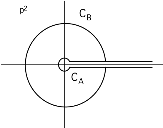
Figure 5: Contours in the $p^{2}$ plane.

Contour $C_{A}$ is evaluated using our knowledge of hadron spectroscopy. Because the contour runs around the real axis, the integral is given by the imaginary part of $G_{n}(p^{2},p^{+})$ - a sum of delta function contributions from hadronic bound states with the quantum numbers of the pion, plus possible multiparticle continuum contributions. To emphasize the lowest-lying state, in this case the pion, we multiply $G_{n}(p^{2},p^{+})$ by the “entire” function $e^{-p^{2}/M^{2}}$, with $M^{2}$ an adjustable mass. Then, a short calculation for the integral along $C_{A}$ gives

$$I_{A}(M^{2}) = \int_{C_{A}}{dp^{2}\over 2\pi iM^{2}}\;G_{n}(p^{2},p^{+})e^{-p^{2}/M^{2}}$$ (34)

$$= ={\left(ip^{+}\right)^{n+1}\over M^{2}}\;\langle x^{n}\rangle\langle x^{0}\rangle+R_{A}\,,$$ (35)

where $\langle x^{n}\rangle$ is the weighted integral of $\phi_{\pi}$ in Eq. (31), and $R_{A}$ is a remainder, associated with higher-mass resonances such as the $A_{1}$, and the continuum. This integral is referred to as a Borel transform.

The corresponding integral $I_{B}(M^{2})$ taken along contour $C_{B}$ is computed quite differently. Along $C_{B}$, the integrand is evaluated far from any resonances, and we may hope that it behaves as it does for Euclidean $p^{2}<0$, where the OPE applies. Rules for its calculation are straightforward but rather technical. The basic structure of the answer, however, is readily expressed as a sum of a perturbative term plus two nonperturbative contributions, from the gluon condensate $\langle G_{\mu\nu}(A)G^{\mu\nu}(A)\rangle_{0}$ and the quark condensate $\langle{\bar{q}}q\rangle_{0}$,

$$I_{B}(M^{2})=h_{I}^{(n)}(M^{2},p^{+})+h_{G^{2}}^{(n)}\langle G^{2}\rangle_{0}+h_{({\bar{q}}q)^{2}}^{(n)}(\langle{\bar{q}}q\rangle_{0})^{2}+R_{B},$$ (36)

where $R_{B}$ represents corrections. All the $h$’s (“coefficient function of the OPE) are computed in perturbation theory.

The values of $M^{2}$ and $s_{0}$ are to be chosen to minimize $R_{A}$ in Eq. (35). Values of $<\bar{q}q>_{0}$ and $<G^{2}>_{0}$ may be found from the analysis of $e^{+}e^{-}\to$ hadrons [29]. Finally the coefficient functions $h^{(n)}$ depend on a renormalization scale $\mu_{0}{}^{2}$. Combining these choices and parameters, and setting $I_{A}=I_{B}$, we may therefore determine $\langle x^{n}\rangle$, or equivalently $\langle\xi^{n}\rangle$, with $\xi=1-2x$ the relative fractional momentum. The CZ wave function in Eq. (27) above was found by fitting its moments to those found by the sum rules.

2.4 Beyond the Pion

2.4.1 Generalizations Most of the developments outlined above for the pion apply as well to electromagnetic form factors for other hadrons, especially baryons [34, 35, 9, 36] and also resonance production, as well as vector mesons and kaons [6, 32, 37, 38]. The form factors of baryons are determined by three-quark valence wave functions, and for both vector mesons and baryons nontrivial spin structure must be taken into account. So long as transverse degrees of freedom may be neglected, however, spin may be described in terms of conserved helicity, where the helicity of a hadron is given by the sum of the helicities of the its partons. A PQCD treatment of violations of helicity conservation has been proposed in [16, 17]. We shall have occasion below to review some of the successes and limitations of this rich constellation of predictions for hadronic form factors.

For example, the wave function of a proton is a sum of terms describing total helicity $\pm 1/2$, times functions $\phi_{i}(x_{1},x_{2},x_{3},\mu^{2})$ with $\sum_{i}x_{i}=1$. The application of evolution analysis to these wave functions shows that asymptotically that have the simple form,

$$\phi^{P}_{ASY}(x_{i})={\rm const.}\times\;x_{1}x_{2}x_{3}\,.$$ (37)

In this case, no readily observed decay amplitude is available to normalize the asymptotic wave function, and hence the proton’s form factor. A Sudakov analysis of the proton wave function and form factor is also possible, with the same general properties as for the pion. [7, 36] It involves two transverse separations, however, and is correspondingly more complex.

Another important difference between the proton and the pion is in the baryonic analogue of Eq. (7) for helicity form factors $G$ (see below), which we may represent schematically as

$$G(Q^{2})=\int dx_{1}dx_{2}\;dy_{1}dy_{2}\;\phi^{P}(y_{j},\mu^{2})\;T_{G}(y_{j},x_{i},Q)\;\phi^{P}(x_{i},\mu^{2})\,,$$ (38)

where $T_{G}$, and hence $G$, is proportional to $Q^{-4}$, and begins at order $\alpha_{s}^{2}$. Here, in contrast to Eq. (7) for the pion, however, the perturbative expansion of the “hard-scattering” function $T_{G}$ receives infrared divergent contributions from regions that resemble the Feynman mechanism, in which one quark carries essentially all of the proton’s momentum, beginning at two loop corrections [9, 10]. Such regions are suppressed by Sudakov corrections. Progress has been made in quantifying this observation for valence PQCD, by introducing transverse degrees of freedom for baryons, as for the pion, but a complete formalism for baryon form factors, even to leading power in $Q^{2}$, remains for the future.

2.4.2 Baryon Helicity Matrix Elements. For use below, let us define electromagnetic helicity matrix elements for nucleons. Taking into account resonance production, an initial state with helicity $\lambda$ = 1/2 may become a final state with $\lambda^{\prime}$ = 1/2 or 3/2. Transitions between a nucleon state ${|N>}$, and final state ${|N^{\prime}>}$ can be expressed in terms of dimensionless helicity matrix elements,

$${G_{H}\ \equiv\ {{1}\over{2M_{N}}}<N^{\prime},\lambda^{\prime}|\epsilon^{\mu}\cdot J_{\mu}|N,1/2>}.$$ (39)

This notation follows [39]. The polarization vectors $\epsilon^{\pm,0}$ correspond to right ($G_{+}$) and left ($G_{-}$) circularly polarized photons and longitudinally ($G_{0}$) polarized photons, respectively. $G_{+},G_{0},G_{-}$ describe transitions in which $\Delta\lambda$ = 0, 1 and 2, respectively. Assuming that helicity is conserved, valence PQCD suggests that $G_{+}\propto QG_{0}\propto Q^{2}G_{-}$. For elastic scattering, since the recoil nucleon has spin 1/2, only the helicity conserving $G_{+}$ ($\Delta\lambda$ = 0 ) and non-conserving $G_{0}$ ($\Delta\lambda$ = 0) contribute.

2.5 Nonasymptotic Form Factors

The valence PQCD results above determine the form factor at very high $Q^{2}$. How high one must be, however, is a matter of debate (see below). It is therefore important to develop treatments of the transition to asymptotic behavior. The evolution of wave functions is a step in this direction, but at moderate $Q^{2}$, it is necessary to apply methods, or develop models that take into account processes that are suppressed even by powers of $Q^{2}$ at high energy. These include the soft processes discussed above.

2.5.1 Sum rules for Form Factors. Refs. [40] and [41], have utilized the sum rule approach to directly obtain form factors, without the intermediate step of determining wave functions. This approach, as described above, depends on the analyticity properties of Green functions that are associated with form factors. It is thus not a dynamical theory of soft or hard interactions, but relies on general properties of QCD, such as the OPE, in addition to perturbative calculations. For a hybrid approach, with features of both QCD sum rules and valence PQCD, see [42].

For the pion form factor the relevant Green function may be expressed as

$$T_{\mu}(p_{1},p_{2})=i^{2}\int e^{-ip_{1}\cdot y+ip_{2}\cdot z}\langle 0|T[J(y)J^{em}_{\mu}(0)J(z)|0\rangle d^{4}zd^{4}y\,,$$ (40)

with $J=J_{0}$ defined as in Eq. (32), and $J^{em}$ the electromagnetic current. In terms of a related scalar amplitude $T$, this Green function possesses a double dispersion relation,

$$T(p^{2}_{1},p^{2}_{2},Q^{2})={{1}\over{\pi^{2}}}\int_{0}^{\infty}ds_{1}\int_{0}^{\infty}ds_{2}\,{{\rho(s_{1},s_{2},Q^{2})}\over{(s_{1}-p_{1}^{2})(s_{2}-p_{2}^{2})}}\,.$$ (41)

The spectral function contains a pion pole which defines the pion form factor, $\rho_{\pi\pi}(s_{1},s_{2},Q^{2})=2\pi^{2}f_{\pi}^{2}F_{\pi}(Q^{2})\delta(s_{1}-m_{\pi}^{2})\delta(s_{2}-m_{\pi}^{2})$, as well as a continuum above the 3-pion threshold, which also includes the broad $A_{1}$ state. The form factor $F_{\pi}$ is extracted by relating the two contours of Fig. 5, this time in both variables $s_{1}$ and $s_{2}$. In [41], the Borel transform is replaced by a simple integral ($M^{2}\rightarrow\infty$), and $s_{0}\sim 8\pi^{2}f_{\pi}^{2}\sim 0.7$GeV² is adjusted to reflect this choice, known as “local duality”. This leads to a relation between $F_{\pi}(Q^{2})$ and the lowest-order perturbative contribution to $\rho$, which may be evaluated to give

$$F_{\pi}(Q^{2})=1-{\left(1+6s_{0}/Q^{2}\right)\over\left(1+4s_{0}/Q^{2}\right)^{3/2}}.$$ (42)

Expanding in inverse powers of $Q$, this expression behaves as $Q^{-4}$ for large momentum transfers, and is thus eventually nonleading compared to the perturbative prediction (22). Nevertheless, as we shall see, it gives a viable fit to the available data, which implies at the least that “soft physics” plays an important role in the charged pion form factor at present energies. Beyond lowest order, $\rho$ includes gluonic corrections, which appear to correspond to the hard gluons of valence QCD. Similar methods have be used to treat baryon form factors [43, 44].

2.5.2 Models. Unfortunately the complexity of soft processes in QCD does not lend them to simple physical models. Their description in terms of fundamental QCD is one of the outstanding theoretical challenges in the theory. There have, however, been useful attempts to bridge the low and high $Q^{2}$ regions with various phenomenological or empirical approaches, concentrating on nucleon form factors.

The generalized vector dominance model (VDM) or hybrid model of [45] begins with the VDM, which yields the requisite low $Q^{2}$ form-factor. Additional terms join VDM form-factors smoothly to PQCD expectations at high $Q^{2}$ ($G_{M}\propto Q^{-4}$ and $G_{E}\propto Q^{-6}$). With the appropriate choice of parameters an excellent agreement with the $G^{P}_{M}$ data is achieved over the entire range of available $Q^{2}$. Agreement with the other elastic form factors, however, turns out to be poor in the light of more recent data.

The Constituent quark model has been been modified, and relativized to extend their validity into the few GeV² region of $Q^{2}$ [46, 47, 19]. For example, in the calculation of hadronic form factors in [19], the constituent quarks, of mass $\sim$ .33 GeV, have wave functions which are solutions to a potential derived from a quark-quark interaction model. In a light cone frame the wave function takes the form $\psi(x,{p_{T}})\sim X(x)P(x,{p_{T}})$. The range of $p_{T}$ in the model wave function effectively has an ultraviolet cutoff so that the one-gluon perturbative parts are not included in the derived form factor. With reasonable choice of $X$ the soft components play an important, and even dominant role over the entire range of measured $Q^{2}$. However, there models are not rigorous enough to make precise predictions.

The diquark model [48, 49, 50] assumes that the baryon distribution function can be expressed in terms of two constituents, a quark and a diquark, which consists of a correlated quark pair. The diquark structure allows for helicity non-conservation, and thus at some level can also account for soft processes. The diquark becomes completely equivalent to the valence PQCD model in the high $Q^{2}$ limit. Its several parameters can be tuned to give a good fit over the entire range of $G^{P}_{M}$, including the transition $Q^{2}$ range.

3 Experimental Status of Hadronic Form Factors

3.1 Pion Form Factors

In this section we will discuss the $\pi^{+}$ and $\pi^{0}$ form factors as obtained in the reactions $p(e,e^{\prime}\pi^{+})n$ and $e^{+}+e^{-}\rightarrow\pi^{0}$, respectively. Given the relative simplicty of the mesonic valence state, we might expect perturbative analysis to apply at lower momentum transfers for pions than for nucleons. We discuss the successes and shortcomings of the valence QCD approach in explaining the data, and also point out important uncertainties in the data itself at high $Q^{2}$.

3.1.1 The Charged Pion Form Factor. The $\pi^{+}$ form-factor is obtained by studying electroproduction on a hydrogen target (see Fig. 6). The aim is to separate the “$t$-channel process”, in which the electron scatters from a nearly on-shell virtual pion emitted from the proton. This $t$-channel cross section, which is due to the exchange of a longitudinal (L) photon, determines the pion form factor, though the relation

$$\sigma_{L}\sim-{{tg^{2}_{\pi NN}(t)}\over{(t-m_{\pi}^{2})^{2}}}F^{2}_{\pi}(Q^{2})\,,$$ (43)

where $t$ is the squared momentum transfer to the nucleon, and $g^{2}_{\pi NN}(t)$ is the $\pi NN$ coupling.

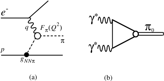
Figure 6: a) Interpretation of t-channel $\pi^{+}$ production in terms of the pion form factor $F_{\pi}$. b) Lowest order diagram for the $\pi^{0}$ form factor.

Nearly all the existing high $Q^{2}$ data, shown in Fig. 7, were obtained at Cornell [51, 52, 53]. Care, however, must be exercized in the interpretation of the higher $Q^{2}$ points, which do not include systematic errors. The reason for this uncertainty is that the separation of $\sigma_{L}$ from the complete cross section requires measurements at different electron scattering angles at the same $Q^{2}$. This “Rosenbluth separation”, was not practical at the highest $Q^{2}$ in this experiment. For $Q^{2}$$>$ 4 GeV²  the (unwanted) transverse cross section was estimated from an extrapolation of low $Q^{2}$ data, and subtracted by hand. Thus, although reliable data exist for $Q^{2}<3$ GeV², the 6.3 and 9.7 GeV² points provide little help in distinguishing between theoretical models.

Figure 7: The form factor of the $\pi^{+}$ meson $Q^{2}F_{\pi}(Q^{2})$ vs $Q^{2}$. The data are from [51, 52, 53]. See the text for comments on the interpretation of the higher $Q^{2}$ data. The dot-dash curves labelled CZ and ASY are obtained from Eq. (39), using $\phi_{CZ}$ and $\phi_{ASY}$ respectively. The dashed curve labelled SR is the direct sum rule result of [43]. The solid curve LS is from [8], using the CZ valence quark distribution amplitude, and including the effects of Sudakov suppression.

There are also important theoretical issues in the extraction of the data. For instance, the struck pion is off-shell, and one must extrapolate to the physical pion pole at $t=-m_{\pi}^{2}$. Uncertainties in the $t$ dependence of $g^{2}_{\pi NN}(t)$ also lead to uncertainties in $F_{\pi}$. In addition, the reliability of high $Q^{2}$ form factors extracted in this manner has been questioned by [54], who claim that other hard, non-resonant processes compete with the $t$-channel process, and may be difficult to separate from it. These objections aside, an important future goal is to extend the pion form factor data to higher $Q^{2}$ [55].

3.1.2 Comparison with Theory. In the valence PQCD framework, the pion form factor may be written in factorized form as in Eq. (7). Treating the hard-scattering at lowest order, with $f_{\pi}\sim$ 93 MeV, we have

$$F_{\pi}(Q^{2})=={16\pi C_{F}\alpha_{s}(\kappa^{2})\over Q^{2}}\left|I\right|^{2}\hskip 18.06749pt{\rm with}\hskip 18.06749ptI=\int_{0}^{1}dx\,{{\phi_{\pi}(x)}\over{x}}\,.$$ (44)

This formula, with a valence quark distribution amplitude derived from QCD sum rules [32], denoted $\phi_{CZ}$, gives a pion form factor in rough agreement with the data as shown in Fig. 7. In obtaining this, the variation in $\alpha_{S}$ was fit to the evaluated data [56], with $\kappa^{2}$ = $Q^{2}$/4. The asymptotic distribution amplitude $\phi_{ASY}$, Eq. (21), which yields Eq. (20), seriously underestimates the data. Refering to Fig. 4, the difference is that $\phi_{CZ}$, Eq. (27), has a “double-hump” structure, concentrated near $x\sim 0$ and $1$, and hence yields a larger value for $I$ than the more central $\phi_{ASY}$. This apparent success inspired many theoretical papers based upon the “QCD sum rule” technique for describing exclusive reactions. The authors of [19, 20] on the other hand, observed that with $\phi_{CZ}$, Eq. (44) is dominated by soft gluon momenta $k^{2}_{g}$ (= $xyQ^{2}$), near the end-point regions discussed above. They argued that Eq. (44), or for that matter PQCD, is invalid in the kinematic regime where data is available, because higher-order perturbative corrections would be uncontrollably large for gluons of such low momenta. If one cuts off the integral in Eq. (44) below a minimum gluon invariant mass, say $k^{2}_{g}\sim.5$ GeV², one derives a much smaller “legal” part of the form factor ( $\sim$ 10 - 20 percent remains for $Q^{2}$ between 5 and 10 GeV² ).

Roughly, proponents of valence PQCD were faced with the dual problems of how to keep the main contributions to the $x$ integral in Eq. (44) away from the endpoints, at the same time enhancing their values relative to the simple use of $\phi_{ASY}$. One way of doing this is to resum a selection of higher-order corrections into the argument of the strong coupling. Choosing $\mu^{2}=xyQ^{2}$ in $T$ in (7) results in a significant enhancement, because the perturbative running coupling grows as its scale decreases. This running coupling, however, diverges for $xyQ^{2}=\Lambda^{2}_{\rm QCD}$, which requires the introduction of a scale below which the coupling is “frozen”. The result is naturally quite sensitive to the cutoff, but it can give a reasonable result without dipping too far into the nonperturbative region [57].

In a related development, it was argued that transverse degrees of freedom should not be neglected, and indeed mimic a gluon effective mass, which suppresses the blowup near $x,y=0$ [58]. We have already seen how Sudakov resummation of transverse degrees of freedom in Eq. (24) results in a naturally self-consistent calculation of the form factor, without cutoffs [8]. In this case, the CZ distribution amplitudes continued to account for the existing data, when the enhancement associated with the running coupling was included. These results for the $\pi^{+}$ form factor are plotted in Fig. 7.

The calculation of [8] has been generalized in [59], who specifically included an “intrinsic” transverse wave function. That is, in Eq. (24) above, they replaced $\exp(-S)\rightarrow\exp(-S)\;\Sigma(x,b)$. Using a model, Gaussian shape for $\Sigma$, they found that this further protected the resulting form factor from the soft region, but also further supressed the hard part of the form factor below the data. Of couse, this proceedure introduced an additional parameter, in the Gaussian, and it included a constituent quark mass.

In an alternatative approach (described in Sec. 2.5.1 above) the direct prediction of $F_{\pi}$ from QCD sum rules, Eq. (42) [41], accounts for most of the measured $F_{\pi}$, without including gluon exchange into its perturbative calculation, even though the resulting expression decays as $Q^{-4}$ at higher $Q^{2}$. In this and other alternatives to the valence quark picture, the apparent scaling with $Q^{2}$ of the present data is interpreted as something of an accident. The extra contribution of a gluon exchanged between quarks, which produces $Q^{-2}$ behavior asymptotically, has been estimated [60], and leads to a modest increase at the highest available $Q^{2}$. These two contributions are referred to as “soft” and “hard” [60], the latter being identified with the valence PQCD prediction.

Other publications continue to focus on the relative importance of soft and hard processes, and in particular how to deal with the difficult soft sector. Examples are [42, 31, 61, 59, 18, 30], who all conclude that soft processes are important for $Q^{2}$ corresponding to the existing data.

Timelike ($s=q^{2}>0$) Pion Form Factor. This is obtained in the reaction $e^{+}+e^{-}\rightarrow\gamma^{*}\rightarrow\pi^{+}+\pi^{-}$. Only one data point exists in the multi-GeV² region, at $s=M^{2}_{J/\psi}\sim 9.6$ GeV², obtained from the ratio $(J/\psi\rightarrow\pi^{+}\pi^{-})/(J/\psi\rightarrow e^{+}e^{-})$ by [62]. This point appears to be more reliable than the higher $Q^{2}$ space-like data. Its calculation is identical to the space-like case in most respects, and it would be useful to obtain timelike data over a range of $Q^{2}$. This process was calculated [63] with valence PQCD techniques, employing evolution and Sudakov suppression, as in [8]. The ratio of experimental timelike to spacelike form factors, about 2, is consistent with the valence PQCD calculation, although the overall normalization is low by a factor of two or more, depending on the light-cone distribution amplitude employed.

3.1.3 The $\pi^{0}$ Form Factor. The $\gamma+\gamma^{*}\rightarrow\pi^{0}$ form factor is expected to be a particularly good test for the pion’s valence distribution amplitude, since at lowest order in the hard scattering it is a pure QED processes (see Fig. 6b). Higher Fock state contributions are suppressed by powers of $\alpha_{s}(Q^{2})/Q^{2}$. In addition, there is no analogue of the “soft”, Feynman mechanism contributions, which require an incoming and an outgoing pion.

Experimentally, the $\pi^{0}$ form factor can be studied via either the Primakoff effect or virtual Compton scattering. The former is accessible in $e^{+}-e^{-}$ colliders, while the latter is more appropriate to fixed target machines. Fig. 8 includes data of the CLEO-II group, [64] which reported measurements up to $Q^{2}$$\sim$ 8 GeV², from reactions $e^{+}e^{-}\rightarrow\pi+X$.

Figure 8: Form factor in the few GeV² range for $\gamma+\gamma^{*}\rightarrow\pi^{0}$. Data for $Q^{2}$ $>$ 3 GeV² are from [64], and lower $Q^{2}$ data from [66]. The dot-dash curve labelled CZ is the result of using $\phi_{CZ}$ in the integral $I$ in Eq. (40), and the solid curve labelled ASY is obtained when using $\phi_{ASY}$. To obtain these curves, Eq. (40) has been modified so that the form factor joins smoothly with the known value at $Q^{2}$ = 0, using a generalization of the prescription of [6]. The horizontal line at the right labelled ASY-limit is the high $Q^{2}$ limit, using $\phi_{ASY}$. The dashed curve labelled SR is the soft form factor obtained directly from QCD sum rules [67].

Working to lowest (zeroth) order in $\alpha_{s}$, by analogy with Eq. (44), the relationship between the $\pi^{0}$ form factor and the valence quark distribution amplitudes is

$$F_{\gamma\gamma\pi^{0}}(Q^{2})={4\over\sqrt{3}Q^{2}}I\,,\hskip 72.26999ptI=\int_{0}^{1}dx\,{{\phi_{\pi}(x)}\over{x}}\,.$$ (45)

A calculation [65] following [8], including Sudakov effects, and an intrinsic transverse distribution amplitude as above,

$$F_{\gamma\gamma\pi^{0}}(Q^{2})=\int dx{{d^{2}b}\over{4\pi}}\phi_{\pi}(x)\Sigma(x,b)\hat{T}_{H}(x,b,Q){\rm e}^{-S(x,b,Q)}\,,$$ (46)

appears to account well for the $\pi^{0}$ form factor. The results with $\phi_{\pi}=\phi_{CZ}$ and $\phi_{ASY}$ are shown in Fig. 8. To compare theory with experiment in this lower $Q^{2}$ region, Eq. (45) has been modified so that the form factor joins smoothly with the known value at $Q^{2}$ = 0, using a generalization of the prescription of [33]. In this case, $\phi_{ASY}$ accounts for the data, while $\Phi_{CZ}$ overshoots it. A recent sum rule computation of this form factor [67] also accounts well for the data. Because the hard-scattering in the $\pi^{0}$ form factor starts, as in Eq. (45), at zeroth order in $\alpha_{s}$, the sum rule and valence PQCD approaches both begin with the same perturbative diagrams. Finally, one may determine the integral $I$ directly by fitting Eq. (45) to the $\pi^{0}$ data, as shown in Fig. 8. The result is close to the value of $I$ for $\phi_{ASY}$.

Comparing the $\pi^{0}$ and $\pi^{+}$ form factors, the success of the asymptotic distribution amplitude in the former suggests that $\phi_{ASY}$ should be used to compute the the valence PQCD contribution to the latter as well. Then, however, the valence contribution with lowest order gluon exchange accounts for less than one half of the $\pi^{+}$ data (see, for instance, [63]). We conclude that, if the charged pion data is accurate at all, either non-valence (soft) contributions, or higher-order contributions in valence PQCD, must play an important role. We note a lack of need for the soft mechanism in the $\pi^{0}$ form factor, which is consistent with these observations. Higher-order hard corrections are also different in the two form factors, however, so it is difficult to draw a final conclusion without further study. We consider, however, that it is likely that the soft mechanism plays an important, and possibly dominant, role in the region of a few GeV² where reliable data exist.

3.2 Nucleon Form Factors

In this section and the next we consider nucleon elastic form factors and transition form factors involving resonant states of nucleons. Since there exist stable on-shell baryon targets, the nucleons, and there are a large variety of final states of spin and isospin, the resonances, a wealth of experimental information can be accessed. Nevertheless, rather limited data exist at high $Q^{2}$.

3.2.1 Nucleon Elastic Form Factors. The elastic electron-nucleon cross section, expressed in terms of the Sachs form factors, is

$${{d\sigma}\over{d\Omega_{e}}}\ =\ {\sigma_{M}f_{rec}}\left({{|G_{E}|^{2}\ +\ \tau|G_{M}|^{2}}\over{1+\tau}}\ +\ 2\tau|G_{M}|^{2}\tan^{2}{\theta/2}\right).$$ (47)

Here, ${\sigma_{M}}$ is the Mott cross section for scattering from a point object, ${f_{rec}}$ $={E^{\prime}/E}$ is a recoil factor, $\tau\ \equiv\ Q^{2}/4M_{N}^{2}$ and $\kappa$ is the anomalous magnetic moment of the nucleon, in nuclear magnetons: ${\rm\kappa_{P}}=1.79$, and ${\rm\kappa_{N}}=-1.91$.

The helicity matrix elements $G_{\pm,0}$, defined above in Sec. 2.4, are related to the Sachs form factors, and the Fermi ($F_{1}$) and Pauli form factors ($F_{2}$) as follows:

$$G_{+}\ = \ {{Q}\over{\sqrt{2}M_{N}}}G_{M}\ =\ {{Q}\over{\sqrt{2}M_{N}}}(F_{1}\ +\ \kappa F_{2})\,,$$ (48)

$$G_{0}\ = \ G_{E}\ =\ F_{1}\ -\ {{Q^{2}}\over{4M_{N}^{2}}}\kappa F_{2}\,.$$ (49)

For elastic scattering from nucleons there are two helicity conserving and two helicity non-conserving form factors, $G^{P}_{M},\,G^{N}_{M}$ and $G^{P}_{E},\,G^{N}_{E}$, respectively. At low $Q^{2}$ (less than one or two GeV²) all the form factors are consistent with a dipole $Q^{2}$ dependence, $1/(1+Q^{2}/M^{2})^{2}$, with $M\sim 0.71$ GeV².

At high $Q^{2}$, valence PQCD predicts that the $Q^{2}$ behavior of the helicity conserving form factors $G^{P}_{M}$ or $G^{N}_{M}$ should follow $\alpha^{2}_{s}(Q^{2})/Q^{4}$ (see Sec. 2.4.1), where we recall that $\alpha_{s}(Q^{2})$ decreases logarithmically in $Q^{2}$. In addition, their magnitudes are determined by relations like (38) using nucleon wave functions, either of the asymptotic form (Eq. (37)), or as found, for instance, from sum rules. The helicity non-conserving form factors should $G^{P,N}_{E}$, should fall as $G^{P,N}_{M}/Q^{2}$ [6]. In the high $Q^{2}$ limit of Eq. (49), $F_{1}\sim G_{M}\propto G_{+}$.

Fig. 9 summarizes what is known experimentally about these four form factors, which were mostly obtained at SLAC. $G^{P}_{M}$ is known best, followed in order by $G^{N}_{M}$, $G^{P}_{E}$ and $G^{N}_{E}$. We will consider each in turn.

Figure 9: The elastic form factors as a function of $Q^{2}$ divided by the dipole shape: a)$G^{P}_{M}$ (spacelike): $\bullet$ - [70], - [68, 71]. b)$G^{P}_{E}$. The curves are: solid [57], dashed [20],dot-dash [45]. $G^{P}_{M}$ (timelike): $\bullet$ - [79], - [80]. b)$G^{P}_{E}$: $\bullet$ [70]. The curves are: dashed [20], dot-dash [45]. c)$Q^{2}F_{2}/F_{1}$: $\bullet$ [70]. The curves are: dashed [20], dot-dash - [45]. d)$G^{N}_{M}$: $\bullet$ [81], [72], $\times$ [73]. The curves are: solid [57], dashed [20], dot-dash [45]. e)$G^{N}_{E}$: $\bullet$ [81], [72], $\times$ [73].

3.2.2 The Proton Magnetic Form Factor. Only $G^{P}_{M}$ has been measured at high $Q^{2}$. In the low $Q^{2}$ limit $G^{P}_{E}$ and $G^{P}_{M}$ are comparable, and can be separated with comparable accuracy by a “Rosenbluth” separation. Separated form factors only exist out to $Q^{2}$ $\sim$ 9 GeV² [68], and unseparated data exist up to $Q^{2}$ $\sim$ 31 GeV² [69]. However, at lower $Q^{2}$ it is observed that $G^{P}_{E}$ is much smaller than $G^{P}_{M}$, and that they are roughly proportional. Since at higher $Q^{2}$ the $G^{P}_{E}$ contribution is kinematically suppressed (see Eq. Ref. (47)), [69] estimated $G^{P}_{M}$, assuming only that $G^{P}_{E}$ does not grow anomalously. The result is presented as a measurement of $G^{P}_{M}$.

Much theoretical work has focussed on the application of the valence PQCD techniques described above to the calculation of the helicity conserving $G^{P}_{M}$ (actually $F_{1}$) [32, 74, 75, 57]. The broad issues are similar to those discussed above for the pion. An advantage relative to the pion, however, is that, because we can scatter electrons from on-shell protons, $G^{P}_{M}$ is relatively unambiguous over a larger range of $Q^{2}$. A disadvantage is that the proton’s three valence quarks make it theoretically more complex.

It was observed quite early that the $Q^{2}$ dependence of $G^{P}_{M}$ is in agreement with quark counting (and hence valence PQCD) predictions. We have already encountered the basic methods and arguments in our discussion for the charged pion form factor. Once again, calculations based on lowest-order gluon exchange and asymptotic distribution amplitudes fall far below the data. After the initial development of sum rule distribution amplitudes [32], however, the situation appeared to improve. This was taken as compelling evidence of the applicability of valence PQCD techniques at measurable $Q^{2}$. This conclusion has been the focus of many papers, sometimes quite contentious, by both proponents and detractors of the use of valence PQCD at accessible $Q^{2}$.

An example is the calculation of [57], based on wave functions derived from QCD sum rules (Sec. 2.3.3). The result of using $\phi^{P}_{CZ}$ from [32] is plotted along with the data in Fig. 9a. Once again, the coupling is forced to run with the virtuality of the exchanged gluons, down to a mass scale at which it is frozen. Good fits to the data were obtained, when this scale (termed an effective gluon mass) is 0.3 GeV. The curve in Fig. 9a is not applicable at low $Q^{2}$, since it is based on leading order PQCD.

This approach has been strongly criticized [19, 20], for the proton as for the pion. The basic question is whether the major contribution to the form factor comes from gluon exchange at low virtuality, where higher-order contributions are not under control. Indeed, sum rules seem to suggest asymmetric nucleon distribution amplitudes, which, as in the case of the pion, enhance contributions from low gluon virtuality. At the very least, this produces strong sensitivity to the mass at which the coupling is frozen, and shakes our confidence in the self-consistency of the valence calculation. Also, it was concluded [76, 77] that the uncertainties in obtaining reliable distribution functions from sum rules, given the experimental uncertainties in the condensates, are so great that the distribution amplitudes are essentially undetermined from sum rules alone. We may also note that the lattice calculation of [26] supports a rather symmetric wave function in the nucleon.

Finally, as for the charged pion form factor, the inclusion of transverse momentum effects [58, 8, 36] stabilizes valence PQCD calculations and improves their self-consistency, while generally reducing them. Thus, Ref. [78], following up on the pion calculation of [59], recalculated $F_{1}$ (or $G^{P}_{M}$) according to the techniques of [8, 36], including intrinsic $k_{\perp}$ componants in the distribution amplitude, $\phi_{P}(x)\rightarrow\phi_{P}(x)\Omega_{P}(x,b)$, with $\Omega$ a Gaussian. In contrast to the pion form factor, the Sudakov resummation for the proton form factor leaves a sensitivity to large $b$ in a corner of the $b,x$ space, necessitating the inclusion of an “infrared” cutoff, that is, a maximum transverse separation in the distribution amplitude. It should be noted, however, that alternate resummations that suppress all large $b$ should be possible, although they have not been explored in the literature. As in the pion case, the extended calculation of [78] reduces the hard scattering form factor significantly below experimental data, for both $\phi^{P}_{CZ}$ and $\phi^{P}_{ASY}$.

$G_{M}^{P}$ at time-like momentum transfer can extend the range of $Q^{2}$ and, together with space-like data, can further constrain theory. The timelike proton form factor has been measured for three values of $Q^{2}$  near 10 GeV² [79]. This, with lower $Q^{2}$ data [80] are also shown in Fig. 9a. As in the pion case, a factor of about two in the ratio for the space-like and time-like form factors is consistent with expectations from valence PQCD [63].

3.2.3 Proton Electric Form Factor. As $Q^{2}$ increases, kinematic suppression of the contribution of $G_{E}^{P}$ in Eq. (47) makes a Rosenbluth separation less and less accurate. As a result, once $Q^{2}$ $\sim$ few GeV², the errors on available data for $G^{P}_{E}$ are significantly worse than for $G^{P}_{M}$. The most recent data [71] obtained by Rosenbluth separation exhibits much smaller errors than previous data, and extends the measured range out to $Q\sim 9$ GeV². The data, shown in Fig. 9b follow a dipole shape over the entire range of $Q^{2}$  to within the limited accuracy.

As indicated above, because $G^{P}_{E}\propto G^{P}_{0}$, which is helicity non conserving, at high $Q^{2}$ the ratio $Q^{2}G^{P}_{E}/G^{P}_{M}$ or $Q^{2}F^{P}_{2}/F^{P}_{1}$ should approach a constant. As seen in Fig. 9c, it appears to do so. This qualitative success of valence PQCD in the 5 – 10 GeV² range makes it attractive to extend the experimental range of accurate $G^{P}_{E}$ data to higher values of $Q^{2}$. A decrease in the ratio $Q^{2}G^{P}_{E}/G^{P}_{M}$ for large $Q^{2}$ of 20 GeV², say, might be a signal that soft processes are still dominant over hard processes in this range.

Of course, at increasing $Q^{2}$ the Rosenbluth separation becomes more difficult. Other methods, involving polarized beam and target or polarized beam and proton recoil polarimeter [82, 83, 84], which measure the ratio $G^{P}_{E}/G^{P}_{M}$, become more favorable. Using such techniques, it will be possible to extend measurements of $G^{P}_{E}$ to higher $Q^{2}$.

3.2.4 Neutron Form Factors. Form factors of neutrons are difficult to obtain, because there are no free neutron targets. Most of the available data were obtained in quasielastic scattering from deuterons, in which the proton contribution is subtracted. This method has intrinsic uncertainies, since one must deconvolute from the quasielastic peak the contributing neutron and proton nuclear wave functions, which must be independently known, as well as the intrusive tails of the inelastic processes, which are also broadened by Fermi motion. This becomes increasingly difficult with increasing $Q^{2}$, as the contribution from quasielastic scattering relative to the inelastic processes decreases dramatically. Eventually, the tail of the inelastic background dominates, and the the extraction of the quasielastic peak becomes extremely sensitive to uncertainties in the modeling of inelastic processes. Thus, at this time data on $G^{N}_{M}$ and $G^{N}_{E}$ are limited to the range $Q^{2}$ $\leq$ 10 GeV² and 4 GeV² respectively.

There are various ways of improving the situation. The detection in coincidence of the struck neutron along with the electron can effectively eliminate the quasielastic proton contribution, and significantly reduce background due to inelastic processes. For $G^{N}_{E}$, which is much smaller than $G^{N}_{M}$, polarization asymmetry techniques can yield the ratio $G^{N}_{E}/G^{N}_{M}$. This method has been employed successfully at lower $Q^{2}$ [85], and is currently planned [86, 87] for the few GeV² range. Neutron form factor data in the GeV² region were obtained at SLAC [72], emploing careful Rosenbluth L/T separations of single arm cross section measurements. The available data are summarized in Fig. 9c and Fig. 9d. The $G^{N}_{M}$ data are consistent with the dipole shape over the entire range of $Q^{2}$, athough there is significant variance between data sets below about 1 GeV². The data for $G^{N}_{E}$ is consistent with zero up to the highest $Q^{2}$, although the errors are quite large.

The value of this data, even though the range is mostly limited to the region where soft processes may still dominate, is quite apparent. All the theoretical non-valence PQCD curves deviate from the data on $G^{N}_{M}$ with increasing $Q^{2}$. Examples shown are the hybrid [45] and the QCD sum rule result of [20]. The constituent quark [47], and vector dominance [88] models also appear to diverge monotonically with increasing $Q^{2}$. The data on $G^{N}_{E}$ clearly eliminates the hybrid model, whereas the VDM and QCD sum rule based calculations are consistant with zero over the $Q^{2}$ range.

To make further use of the selectivity of the nucleon form factors, it will be important to obtain data on $G^{N}_{E}$, $G^{N}_{M}$ and $G^{P}_{E}$ at $Q^{2}$ greater than the present limits. Such experiments for $G^{N}_{M}$ and $G^{P}_{E}$ have been proposed for future facilities [89, 84]. For $G_{M}^{P}$ at least, its scaling as $Q^{-4}$ over such a large range suggests that valence PQCD is relevant to its description. The soft mechanism may, however, also play an important role, especially at moderate $Q^{2}$. The clarification of this role is an important project for theory and experiment.

Only global tests involving all available form factors can hope to seriously select among varying points of view. We stress the importance of measuring the helicity non-conserving form factors to as high $Q^{2}$ as possible, since in valence PQCD they are driven by non-leading processes, and therefore offer important constraints on the relative importance of soft and hard processes with varying $Q^{2}$.

3.3 Baryon Resonance Amplitudes and Form Factors

The study of transition form-factors to excited baryons at high $Q^{2}$ can make an important contribution to our knowledge of hadronic structure. Fig. 10 shows the virtual photon cross section at $Q^{2}$= 1 GeV² as a function of baryon invariant mass $W$. For $W\ <\ 2$ GeV, the most significant feature is the existence of three maxima, known as the first, second and third resonance regions. In this interval there are about 20 known resonances. These are denoted $L_{2I,2J}(W)$, where $L$ is the angular momentum of the single pion decay, and $I$ and $J$ are respectively the resonance isospin and spin. However, except for the first, which is due to the $\Delta$(1232) the resonances are largely overlapping, even with a significant non-resonant underlay. In future programs, the separation of the contributing electromagnetic multipoles will require measurement of exclusive reactions such as ${\rm(e,e^{\prime}\pi)\ and\ (e,e^{\prime}\eta)}$ to as high $Q^{2}$ as possible, with polarized beams and targets.

Figure 10: The virtual photon cross section for proton excitation at $Q^{2}$= 1 GeV². The data are reconstructed from an evaluation by [90]. The known contributing states are indicated at the bottom by vertical lines. The largest contributing states are indicated by long vertical lines.

The second resonance region is dominated by two strong negative parity states, the $D_{13}(1520)$ and the $S_{11}(1535)$. At low $Q^{2}$ ( $<$ 1 GeV²) the $D_{13}(1520)$ is dominant, whereas at higher $Q^{2}$ ( $>$ 3 GeV²) the $S_{11}(1535)$ dominates. The Roper resonance, the $P_{11}(1440)$, has not yet been definitely observed at $Q^{2}$ $>$ 0, but is of considerable interest since there is speculation regarding its character [91]. In the third resonance region, the largest excitation at low $Q^{2}$ is the $F_{15}(1680)$. The relative strength of the other states is not well determined, especially at increasing $Q^{2}$. At low $Q^{2}$ the excitations indicated in Fig. 10 have been rather successfully described in terms of the constituent quark model.

The current experimental situation is that exclusive ${\rm(e,e^{\prime}\pi)\ and\ (e,e^{\prime}}$ $\eta)$ data exist only up to $Q^{2}$ = 4 GeV². Although there is a total absence of exclusive data above $Q^{2}$=3 GeV², there are inclusive data in the resonance region obtained mostly at SLAC (see references in [92]). Although the statistical accuracy becomes poor at high $Q^{2}$, the three peaks near $W$ = 1232, 1535 and 1680 MeV remain prominent, with the $\Delta(1232)$ obviously decreasing with increasing $Q^{2}$ relative to the other two. After subtraction of phenomenological non-resonant backgrounds the peaks were fit with resonance functions ([92]) to extract transverse form factors, $|G_{T}(Q^{2})|^{2}\equiv(|G_{+}|^{2}+|G_{-}|^{2})/2\tau$, where $\tau\equiv Q^{2}/4M_{n}^{2}$.

The form factors, are shown in Fig. 11, relative to a dipole shape. Also shown at lower $Q^{2}$ are form factors extracted from data obtained earlier from exclusive ${(e,e^{\prime},p)\pi^{\circ}}$ and ${(e,e^{\prime},p)\eta}$ experiments.

Figure 11: The quantity ${G_{T}/G_{dipole}}$ verses $Q^{2}$ for the elastic form factor (a), and for transitions to the first (b), second (c) and third (d) resonances respectively, with $G_{dipole}=2.79(1+Q^{2}/.71)^{-2}$ in (a) and $3(1+Q^{2}/.71)^{-2}$ in (b-d). The first resonance (b) is the $\Delta$(1232) (the $P_{33}(1232)$). The second resonance ( c) at $Q^{2}$ above about 3 GeV² is dominated by the S₁₂(1535). The third resonance at low $Q^{2}$ is dominated by the F₁₅(1680). The fits for ${G_{T}}$ were based on inclusive data referenced in [93, 92]. and selected data from [95]. The elastic proton form factor $G_{Mp}$ is shown in a). Also shown at lower $Q^{2}$, denoted by ($\times$), are form factors derived from amplitudes obtained from exclusive ${(e,e^{\prime},p)\pi^{0}}$ and ${(e,e^{\prime},p)\eta}$ data. The dashed curves are the result of the local duality sum rule calculations of [43] and [44] for the elastic and $\Delta(1232)$ transitions respectively. The solid curve in a) is the $G_{Mp}$ result of the PQCD sum rule calcutation of [57] employing $\phi_{CZ}$. The solid lines at the lower right in b) and c) are the result of the PQCD calculation of [39] using $\phi_{CZ}$ for the $\Delta(1232)$ and $S_{12}$(1535) respectively.

Fig. 11 shows that the form factors obtained for the second and third resonance regions are consistent with a $Q^{-4}$ dependence, although with large statistical uncertainty. On the other hand, the $\Delta(1232)$ form factor is decreasing relative to both the elastic as well as the second and third resonances. Since this result is obtained from inclusive data there are systematic uncertainties in the extraction [94], and more recent analysis of the available data [95] indicates the extent in $Q^{2}$ of the decrease is yet resolved.

3.3.2 $\Delta$(1232): Transition Multipoles Since the $\Delta(1232)$ has $J=3/2$ there are three contributing multipoles, $E_{1+},M_{1+}$, and $S_{1+}$ whose relative contributions are model dependent. Thus, this is a favorable case for studying models of baryon structure. At low $Q^{2}$ in a pure $SU(6)$ non-relativistic CQM the $N\rightarrow\Delta$ transition is purely $M_{1+}$ in character, involving a single-quark spin-flip with $\Delta L$ = 0. An $E_{1+}$ contribution is not permitted, since the $\Delta$ and $N$ are both in $L=0$ states, which cannot be connected by an operator involving $L\ >\ 0$. The addition of a residual quark-quark color magnetic interaction adds higher $L$ components to the $\Delta$ wave function, and thus introduces a small $E_{1+}$ component, of perhaps a few percent. At $Q^{2}$= 0 the experimental data supports the constituent quark model prediction of $M_{1+}$ dominance extremely well. Recent data [96] bears this out. The data from from Mainz [96] reports a ratio $E_{1+}/M_{1+}=-.025\pm.002\pm.002$. This ratio remains very small up to $Q^{2}$ about 1 GeV², beyond which there is very little data. There exist some earlier data at $Q^{2}$= 3 GeV² [97], which has been evaluated by [98], suggesting that $E_{1+}/M_{1+}$ is increasing, but with large errors, ${\rm Re}(E_{1+}/M_{1+})=0.06\pm 0.02\pm.03$, and we must conclude that the magnitude of $E_{1+}/M_{1+}$ at $Q^{2}$ = 3 GeV² remains uncertain. Recently [99] exclusive data were obtained at CEBAF at $Q^{2}$ = 3 and 4 GeV², for the $\Delta(1232)$ and $S_{11}(1535)$, but at the time of writing the analysis is not complete.

At high $Q^{2}$, valence PQCD predicts that only helicity concerving amplitudes should contribute. The multipole amplitudes for single pion production may be expressed in terms of helicity conserving and non-conserving amplitudes as follows:

$$\Delta\lambda\ = \ 0\ :\ A_{1+}\ =\ (3/2)\;M_{1+}\ +\ (1/2)\;E_{1+}$$ (50)

$$\Delta\lambda\ = \ 2\ :\ B_{1+}\ =\ E_{1+}\ -\ M_{1+}$$ (51)

$$\Delta\lambda\ = \ 1\ :\ C_{1+}\ =\ (2Q^{2}/p^{*}_{\pi})\;S_{1+}\,,$$ (52)

where $p^{*}_{\pi}$ is the c.m. pion momentum. Thus, helicity conservation implies $B_{1+}\ =\ 0$, or $E_{1+}\ =\ M_{1+}$. This is quite different from the low $Q^{2}$  situation.

QCD sum rule techniques were applied in [100], to calculate the distribution functions for the $\Delta$(1232) excitation. The CZ [32] proton wave function yields a small transition form factor, $Q^{4}G_{T}(Q^{2})\sim 0.07$ asymptotically. This can be traced to a cancellation in the leading order term of the matrix elements connecting the symmetric $\Delta$(1232) distribution amplitude, with the symmetric and antisymmetric proton distribution amplitude respectively. Schematically, $|\langle\phi_{\Delta}|T_{H}|\phi^{P}_{S}\rangle\ +\ \langle\phi_{\Delta}|T_{H}|\phi^{P}_{A}\rangle|$ is much smaller than either alone.

If the leading amplitude of the P $\rightarrow$ $\Delta$ transition is indeed small, the anomalous shape of the transition form factor might be explained as follows. At high $Q^{2}$, the leading order helicity conserving amplitude dominates over the helicity non-conserving amplitude. That is, $A_{1/2}>>A_{3/2}$. A suppression of the $A_{1/2}$ amplitude at all $Q^{2}$ due to the cancellation of the symmetric and antisymmetric matrix elements, might then result in the dominance of the $A_{3/2}$ amplitude over a larger range of $Q^{2}$ than otherwise expected, and ${Q^{4}G_{T}(Q^{2})}$ would decrease as a function of $Q^{2}$. In fact the evidence that $E_{1+}/M_{1+}$ is still small for $Q^{2}$ up to 3 GeV², is consistent with the dominance of non-leading processes.

Recently [44] the local duality procedure was applied to the $\Delta(1232)$ form factor, and it was found, as in the pion case, that the form factor in the few GeV² region can be accounted for by purely soft processes (see Fig. 10). However, it then falls significantly below the experimental values at higher $Q^{2}$, which might be evidence that hard processes are playing an increasing role.

It will be interesting in the future to determine whether ${Q^{4}G_{T}(Q^{2})}$ does indeed level off above $Q^{2}$= 10 GeV², and where the $E_{1+}$ amplitude becomes comparable to the $M_{1+}$. This would support the valence PQCD description.

3.3.3 The Second Resonance. Fig. 11 shows that at high $Q^{2}$ the form factor for the peak at W $\sim$ 1535 MeV approaches the $Q^{-4}$ dependence predicted by valence PQCD. Although the $D_{13}(1520)$ is dominant at $Q^{2}$ = 0, there is a crossover and the $S_{11}(1535)$ dominates the $D_{13}(1520)$ at $Q^{2}$ $\sim$ few GeV² [97]. Another unique feature of the $S_{11}(1535)$ is that it is the only excited state with a large $\eta$ decay branching ratio ($\sim 50\%$), so that experimentally it is easily is isolated.

Ref. [100] presents a calculation of the ${proton\rightarrow\ S_{11}}$ transition form factor in the valence PQCD framework. The result is a behavior similar to the elastic form factor. Although the results are about a factor of two lower than the data, the authors remark that theoretical uncertainties in the distribution functions, and higher order contributions to $\alpha_{s}$ are probably great enough to account for these discrepancies.

3.3.4 The Third Resonance. Fig. 11 shows that at high $Q^{2}$ the form factor for the peak near W = 1680 MeV is consistent with the predicted $Q^{-4}$ behavior. The errors are large, however, and it is not clear how many resonances are contributing to this peak. The potential for obtaining separated resonance amplitudes at high $Q^{2}$ with exclusive reactions is very good. This is particularly true since it has been demonstrated [101, 93, 102], that the non-resonant background diminishes with $Q^{2}$ at approximately the same rate as the resonances.

3.3.5 Duality. A very interesting concept is that of duality between resonances and the non-resonance continuum in the $W$ region where they overlap. One observes [101] that the rate of decrease with $Q^{2}$ of the resonance cross sections approximately follows the extrapolation of deep-inelastic scaling into the resonance region, suggesting that both processes are related by the same underlying physics. Later, this was put on firmer ground, and it was shown that leading logarithmic corrections extend the duality range in $Q^{2}$  [103, 104]. However, all of this is based on analyses of inclusive data, which cannot effectively separate non-resonance from resonance contributions. In order to access this very fundamental result one really needs to have a clean separation of resonance and non-resonance data over a large range of $Q^{2}$, which can only be accomplished by the measurement of exclusive reactions.

4 Conclusions

As seen, much work remains in both experiment and theory. Valence PQCD and factorization appear to be an attractive starting point for treating high $Q^{2}$ form factors, although how high $Q^{2}$ must be for valence PQCD to dominate remains controvertial, and most probably depends on the specific reaction. Opinions on this matter vary strongly, from those who maintain that the required $Q^{2}$ is much higher than is likely to be experimentally accessible in the forseeable future, to those who believe that valence PQCD is already applicable at $Q^{2}$ as low as a few GeV². We suggest that the quality and extent of existing data does not allow a definitive conclusion, but that soft non-perturbative processes probably play an important role for much of the existing data. On the other hand, given the complexity of QCD, there is a need for further theoretical work, based on fundamental principles of QCD, to deal with the soft, or Feynman mechanism. Indeed, it may be possible to express form factors in the transition region as a sum over valence PQCD and Feynman mechanism contributions, with the hard-scattering imbedded in the latter treated with PQCD methods. For the truly soft region, lattice calculations may play an increasing role in the future [26, 27].

On the experimental side, one must push the frontiers to as high $Q^{2}$ as technically feasible, to provide data which has the best chance of testing these ideas. One should also go beyond the experiments which merely test constituent scaling, to those which test other central tenets of theory, such as helicity conservation. Such work has now begun at CEBAF, and may be further extended by a proposed European facility, ELFE [105] In summary, this area appears to offer some of the most interesting theoretical and experimental challanges for the next decade.

ACKNOWLEDGEMENTS: The authors wish to acknowledge and thank P. Bosted and A. Radyushkin for their valuable assistance. This work was supported in part by the National Science Foundation under grants PHY-9507412 and PHY-930988.

References

- [1] Hofstadter R. Rev. Mod. Phys. 28:215 (1956)
- [2] Feynman RP. 1979. Photon-Hadron Interactions Reading: Benjamin.
- [3] Brodsky SJ, Lepage GP. in Quantum Chromodynamics, ed. AH Mueller, Singapore: World Scientific.
- [4] Farrar GR, Jackson DR. Phys. Rev. Lett. 43:246 (1979)
- [5] Efremov AV, Radyushkin AV. Phys. Lett. 94B:245 (1980)
- [6] Lepage GP, Brodsky SJ. Phys. Rev. D22:2180 (1980)
- [7] Botts J, G. Sterman Nucl. Phys. B325: 62 (1989)
- [8] Li H-N, Sterman G. Nucl. Phys. B381:129 (1992)
- [9] Duncan A and Mueller AH. Phys. Rev. D21:1636 (1980)
- [10] Mueller AH. Phys. Rep. C73:237 (1981)
- [11] Brodsky SJ. 1996. Presented at Orbis Scientiae, Miami Beach, FL. hep-ph/9604391
- [12] Brodsky SJ, Farrar GR. Phys. Rev. Lett.31:1153 (1973)
- [13] Matveev VA, Muradian RM, Tavkhelidze AN. Nuovo Cim. Lett. 7:719 (1973)
- [14] Dittes FM, Radyushkin AV. Phys. Lett. 134B:359( 1984)
- [15] Braaten E, Tse S-M. Phys. Rev. D35:2255 1987)
- [16] Jain P, Ralston, JR. Proc. Am. Phys. Soc. Div. Part. & Fields, 7th, pp 1045-1047 Fermilab. Singapore: World Scientific
- [17] Gousset T, Pire B, Ralston JP. Phys. Rev. D53:1202 (1996)
- [18] Wang SW Kisslinger LS. Phys. Rev. D54:5890 (1996)
- [19] Isgur N, Llewellyn-Smith CH. Nucl. Phys. B317:526 (1989)
- [20] Radyushkin AV. Acta Phys. Pol. B15:403 (1984)
- [21] Muller D. Phys. Rev. D51:3855 (1995)
- [22] Efremov A.V. and Radyushkin A.V., Theor. Math. Phys. 42:97 (1980).
- [23] Collins JC, Soper DE. Nucl. Phys. B193:381 (1981)
- [24] Jain P, Pire, B, Ralston JP. Phys. Rep. 271:67 (1996)
- [25] Cao F-G, Huang T, Ma B-Q. Phys. Rev. D53:6582 (1996)
- [26] Martinelli G, Sachrajda CT. Phys. Lett. B217: 319 (1989)
- [27] Burkardt M, Grandy JM Negele JW. Ann. Phys. 238:441 (1995)
- [28] Shuryak, E. Rev. Mod. Phys. 65:1 (1993)
- [29] Shifman M, Vainstein AI, Zakharov, VI. Nucl. Phys. B147: 385, 448, 519 (1979)
- [30] Lee SH, T.Hatsuda T, Miller GA. Phys. Rev. Lett. 72:2345 (1994)
- [31] Chibisov B, Zhitnitsky AR. Phys. Rev. D52:5273 (1995)
- [32] Chernyak VL, Zhitnitsky AR. Phys. Rep. 112:173 (1984).
- [33] Brodsky SJ, Frishman Y, Lepage GP, Sachrajda C. Phys. Lett. 91B:239 (1980)
- [34] Lepage GP, Brodsky SJ. Phys. Rev. Lett. 43:545 (1979)
- [35] Aznauryan IF, Esaybegyan SV, Ter-Isaakyan NL. Phys. Lett. 90B:151 (1980)
- [36] Li H-N. Phys. Rev. D48:4243 (1993)
- [37] Ji C-R, Farhang A. Phys. Rev. D42:3764 (1990)
- [38] Agaev S. Mod. Phys. Lett. A10:2009 (1995)
- [39] Carlson CE. Phys. Rev. D34:2704 (1986)
- [40] Ioffe BL, Smilga AV. Nucl. Phys. B216:373 (1982)
- [41] Nesterenko VA, Radyushkin AV. Phys. Lett. 115B:410 (1982)
- [42] Braun V, Halperin I. Phys. Lett. B328:457 (1994)
- [43] Nesterenko VA, Radyushkin AV. Phys. Lett. 128B: 439 (1983)
- [44] Belyaev VM, Radyushkin AV. Phys. Rev. D53:6509 (1996)
- [45] Gari M, Krumpelmann W. Phys. Lett. B173:10 (1986)
- [46] Dziembowski Z. Phys. Rev. D37:768 (1988)
- [47] Chung PL, Coester F. Phys. Rev. D44:229 (1991)
- [48] Anselmino M, Kroll P, Pire B. Z. Phys. C36:89 (1987)
- [49] Dziembowski Z, Franklin J. Phys. Rev. D42:905 (1990)
- [50] Kroll P, Schurmann M, Schweiger W. Z. Phys. A342:429 (1992)
- [51] Bebek CJ et al. Phys. Rev. D13:25 (1976)
- [52] Bebek CJ et al. Phys. Rev. Lett. 37:1326 (1976)
- [53] Bebek CJ et al. Phys. Rev. D17: 1693 (1978)
- [54] Carlson CE, Milana J. Phys. Rev. Lett. 65:246 (1979)
- [55] Mack D. in “Workshop on CEBAF at higher energies” N. Isgur and P. Stoler eds. CEBAF pp. 243
- [56] Particle Data Group Phys. Rev. D54:1-I (1996)
- [57] Ji C-R, Sill AF, Lombard-Nelson RM, Phys. Rev. D36:165 (1987)
- [58] Hansper J, Eckert R, Gari M. Z. Phys. A 341:339 (1992)
- [59] Jakob R, Kroll P. Phys. Lett. B315:463 (1993)
- [60] Radyushkin AV. 1994. in “Workshop on CEBAF at higher energies” N. Isgur and P. Stoler eds. CEBAF pp. 273
- [61] Kislinger LS, Wang SW. Nucl. Phys. B399:63 (1993)
- [62] Milana J, Nussinov S, Olsson MG. Phys. Rev. 71:2533 (1993)
- [63] Gousset T, Pire B. Phys. Rev. D51:15 (1995)
- [64] Savinov V. 1995. presented at Workshop on Photon-photon Collisions (PHOTON95), 10th, Sheffield, England. hep-ex/9508004
- [65] Kroll P, Raulfs M. Phys. Lett. B387:848 (1996)
- [66] Behrens HJ et al. Z. Phys. C49:401 (1991)
- [67] Radyushkin AV, Ruskov R. Phys. Lett. B374:173 (1996)
- [68] Sill AF et al. Phys. Rev. D48:29 (1993)
- [69] Arnold RG et al. Phys. Rev. Lett. 57:174 (1986)
- [70] Walker RC et al. Phys. Rev. D49:5671 (1994)
- [71] Andivahis L et al. Phys. Rev. D50:5491 (1994)
- [72] Lung A et al. Phys. Rev. Lett. 70:718 (1994)
- [73] Rock S et al. Phys. Rev. D46:24 (1992)
- [74] King ID, Sachrajda CT. Nucl. Phys. B279:785 (1987)
- [75] Gari M, Stefanis NG. Phys. Rev. D35:1074 (1987)
- [76] Eckardt R, Hansper J, Gari MF. Phys. Rev. D50:R26 (1994)
- [77] Eckardt R, Borg J, Gari MF. Z. Phys. A350:349 (1995)
- [78] Bolz J, Jakob R, Kroll P, Bergmann M, Stefanis NG. Z. Phys. C66:267 (1995)
- [79] Armstrong TA et al. Phys. Rev. Lett. 70:1212 (1993)
- [80] Bardin G et al. Phys. Lett. B257:514 (1991)
- [81] Bartel W et al. Nucl. Phys. B58:429 (1973)
- [82] Bauer TS et al. 1992. in The ELFE Project: Proceedings. J. Arvieux and E. De Sanctis eds. Italian Physical Society Bologna p. 113
- [83] Perdrsat CF et al. CEBAF experiment E-93-027 (1993)
- [84] E. Voutier E et al. 1994. in “Workshop on CEBAF at higher energies” N. Isgur and P. Stoler eds. CEBAF pp. 295
- [85] Eden T. et al. Phys. Rev. C50:R1749 (1994)
- [86] Madey M et al. CEBAF experiment E-93-038 (1993)
- [87] Day D et al. CEBAF experiment E-93-025 (1993)
- [88] Hohler G et al B114:505 (1976)
- [89] Brooks W. 1994. in “Workshop on CEBAF at higher energies” N. Isgur and P. Stoler eds. CEBAF pp. 197
- [90] Brasse FW et al. Nucl. Phys. B110:410 (1976)
- [91] Li Z, Burkert V, Li Zh. Phys. Rev. D46:70 (1992)
- [92] Stoler P. Phys. Rep. 226:103 (1993)
- [93] Stoler P, Phys. Rev. Lett. 66:1003; Phys. Rev. D44:73 (1991)
- [94] R.M. Davidson and N.C. Mukhopadhyay Phys. Lett. B353: 131 (1995).
- [95] Keppel C. 1994. in “Workshop on CEBAF at Higher Energies” N. Isgur and P. Stoler eds. CEBAF pp. 237
- [96] Beck R et al. Phys. Rev. Lett. 78:606 (1997)
- [97] Haidan R. PhD thesis Univ. of Hamburg, unpublished
- [98] Burkert V, Elouadrhiri L. Phys. Rev. Lett. 75:3614 (1995)
- [99] CEBAF experiment 94-014, private communication
- [100] Carlson CE, Poor JL. Phys. Rev. D38:2758 (1988)
- [101] Bloom ED, Gilman FJ. Phys. Rev. Lett. 25:1140 (1970) Phys. Rev. D4:2901 (1971)
- [102] Carlson CE, Mukhopadhyay NC. Phys. Rev. D41:2343 (1990)
- [103] Carlson CE, Mukhopadhyay NC. Phys. Rev. D47:1737 (1993)
- [104] Carlson CE, Mukhopadhyay NC. Phys Rev. Lett. 74:1288 (1995)
- [105] J. Arvieux and E. De Sanctis eds. 1992. The ELFE Project: Proceedings. Bologna: Italian Physical Society