Equilibrium and Non-Equilibrium Hard Thermal Loop Resummation in the Real Time Formalism

Abstract

We investigate the use of the hard thermal loop (HTL) resummation technique in non-equilibrium field theory. We use the Keldysh representation of the real time formalism (RTF). We derive the HTL photon self energy and the resummed photon propagator. We show that no pinch singularities appear in the non-equilibrium HTL effective propagator. We discuss a possible regularization mechanism for these singularities at higher orders. As an example of the application of the HTL resummation method within the RTF we discuss the damping rate of a hard electron.

I Introduction

Perturbation theory for gauge theories at finite temperature suffers from infrared singularities and gauge dependent results for physical quantities. These problems are avoided by using an effective perturbation theory (Braaten-Pisarski method [1]) which is based on the resummation of hard thermal loop (HTL) diagrams into effective Green functions. This powerful method was derived within the imaginary time formalism (ITF). Using resummed Green functions, medium effects of the heat bath, such as Debye screening, collective plasma modes, and Landau damping, are taken into account. The HTL resummation technique has been applied to a number of interesting problems, in particular to the prediction of signatures and properties of a quark-gluon plasma (QGP) expected to be produced in relativistic heavy ion collisions (for a review see [2]).

However, the use of thermal field theories for describing a QGP in nucleus-nucleus collisions is restricted by the fact that at least the early stage of such a collision leads to a fireball, which is not in equilibrium. It is not clear if a complete thermal and chemical equilibrium will be achieved later on. Hence, non-equilibrium effects in a parton gas should be considered for predicting signatures of QGP formation and for obtaining a consistent picture of the fireball. This can be done in the case of a chemically non-equilibrated parton gas by means of rate equations [3] or more generally by using transport models [4]. However, these approaches are based on a semiclassical approximation. In particular, infrared divergences have to be removed phenomenologically. Therefore it is desirable to derive a Green function approach including medium effects as in the case of the HTL resummation. For this purpose one has to abandon the ITF, which is restricted to equilibrium situations. The real time formalism (RTF), on the other hand, can be extended to investigate non-equilibrium systems [5, 6].

The RTF involves choosing a contour in the complex energy plane which fulfills the Kubo-Martin-Schwinger boundary condition and contains the real axis [5]. This leads to propagators and self energies which are given by $2\times 2$ matrices. The choice of the contour is not unique. We will adopt the Keldysh or closed time path contour, which was invented for the non-equilibrium case [5]. In particular, we will demonstrate the usefulness of the Keldysh representation [7] based on advanced and retarded propagators and self energies and show how potentially dangerous terms (pinch singularities) [8] in non-equilibrium are treated easily within this representation.

In the next section we review the Keldysh representation. In section 3, we discuss the equilibrium calculation. We consider QED and give the results of the real time calculation, in the HTL approximation, of the photon self energy, the resummed photon propagator, and the electron damping rate. The results are, of course, identical to those of the ITF, which demonstrates that although the HTL resummation scheme was derived within the ITF, the result is independent of the choice of contour. In section 4, we extend the HTL resummation technique to off-equilibrium situations by following the equilibrium calculations outlined in section 3. We show that no pinch singularities appear in the non-equilibrium HTL effective propagator.

II Keldysh representation

In this section we review the Keldysh representation of the RTF. The bare propagator for bosons reads [6]

$$D(K)=\left(\begin{array}[]{cc}\frac{1}{K^{2}-m^{2}+i\epsilon}&0\\ 0&\frac{-1}{K^{2}-m^{2}-i\epsilon}\\ \end{array}\right)-2\pi i\,\delta(K^{2}-m^{2})\>\left(\begin{array}[]{cc}n_{B}(k_{0})&\theta(-k_{0})+n_{B}(k_{0})\\ \theta(k_{0})+n_{B}(k_{0})&n_{B}(k_{0})\\ \end{array}\right),$$ (1)

where $K=(k_{0},{\bf k})$, $k=|{\bf k}|$, $\theta$ denotes the step function, and the distribution function is given by $n_{B}(k_{0})=1/[\exp(|k_{0}|/T)-1]$ in the equilibrium case.

For fermions the bare propagator can be written as

$$S(K)=(K\!\!\!\!/\,+m)\> \left[\left(\begin{array}[]{cc}\frac{1}{K^{2}-m^{2}+i\epsilon}&0\\ 0&\frac{-1}{K^{2}-m^{2}-i\epsilon}\\ \end{array}\right)\right.$$ (7)

$$+2\pi i\,\delta(K^{2}-m^{2})\>\left.\left(\begin{array}[]{cc}n_{F}(k_{0})&-\theta(-k_{0})+n_{F}(k_{0})\\ -\theta(k_{0})+n_{F}(k_{0})&n_{F}(k_{0})\\ \end{array}\right)\right],$$

where the Fermi distribution is given by $n_{F}(k_{0})=1/[\exp(|k_{0}|)+1]$ in equilibrium. The components of these propagators are not independent, but fulfill the relation

$$G_{11}-G_{12}-G_{21}+G_{22}=0,$$ (8)

where $G$ stands for $D$ or $S$.

By an orthogonal transformation of these $2\times 2$ matrices we arrive at a representation of the propagators in terms of advanced and retarded propagators which was first introduced by Keldysh [7]. The three independent components of this representation are defined as [6]

$$G_{R} = G_{11}-G_{12},$$ (9)

$$G_{A} = G_{11}-G_{21},$$ (10)

$$G_{F} = G_{11}+G_{22}.$$ (11)

The inverted relations read

$$G_{11} = \frac{1}{2}\,(G_{F}+G_{A}+G_{R}),$$ (12)

$$G_{12} = \frac{1}{2}\,(G_{F}+G_{A}-G_{R}),$$ (13)

$$G_{21} = \frac{1}{2}\,(G_{F}-G_{A}+G_{R}),$$ (14)

$$G_{22} = \frac{1}{2}\,(G_{F}-G_{A}-G_{R}).$$ (15)

Similar relations to (8) and (11) hold for the self energies [9]:

$$\Pi_{11}+\Pi_{12}+\Pi_{21}+\Pi_{22}=0$$ (16)

and

$$\Pi_{R} = \Pi_{11}+\Pi_{12},$$ (17)

$$\Pi_{A} = \Pi_{11}+\Pi_{21},$$ (18)

$$\Pi_{F} = \Pi_{11}+\Pi_{22},$$ (19)

where $\Pi$ stands for the self energy of a boson or fermion.

Using (1) and (7) in (11) the bare propagators of the Keldysh representation are given by

$$D_{R}(K) = \frac{1}{K^{2}-m^{2}+i\,\mbox{sgn}(k_{0})\epsilon},$$ (20)

$$D_{A}(K) = \frac{1}{K^{2}-m^{2}-i\,\mbox{sgn}(k_{0})\epsilon},$$ (21)

$$D_{F}(K) = -2\pi i\,[1+2n_{B}(k_{0})]\,\delta(K^{2}-m^{2})$$ (22)

for bosons and

$$S_{R}(K) = \frac{K\!\!\!\!/\,+m}{K^{2}-m^{2}+i\,\mbox{sgn}(k_{0})\epsilon},$$ (23)

$$S_{A}(K) = \frac{K\!\!\!\!/\,+m}{K^{2}-m^{2}-i\,\mbox{sgn}(k_{0})\epsilon},$$ (24)

$$S_{F}(K) = -2\pi i\,(K\!\!\!\!/\,+m)\,[1-2n_{F}(k_{0})]\,\delta(K^{2}-m^{2})$$ (25)

for fermions. The bare propagators $D_{F}$ and $S_{F}$ can be written also as

$$D_{F}(K) = [1+2n_{B}(k_{0})]\,\mbox{sgn}(k_{0})\,[D_{R}(K)-D_{A}(K)],$$ (26)

$$S_{F}(K) = [1-2n_{F}(k_{0})]\,\mbox{sgn}(k_{0})\,[S_{R}(K)-S_{A}(K)].$$ (27)

In the non-equilibrium case, all of these equations are valid, with the equilibrium distribution functions ($n_{B},\,\,n_{F}$) replaced by non-equilibrium distribution functions ($f_{B},\,\,f_{F}$) which depend on the four momentum and the space-time coordinate [6].

Now we consider the situation for full (resummed) propagators. In equilibrium, (27) is valid for full propagators as a consequence of the dissipation-fluctuation theorem [9]. The polarization tensor satisfies,

$$\Pi_{F}(K)=[1+2n_{B}(k_{0})]\,\mbox{sgn}(k_{0})\,[\Pi_{R}(K)-\Pi_{A}(K)]$$ (28)

for bosons, and for fermions we have to replace $n_{B}$ by $-n_{F}$. Out of equilibrium however, the situation is more complicated. Equations (27) and (28) are not satisfied by resummed propagators out of equilibrium. Additional terms occur which appear to give rise to pinch singularities. In section 4 we will discuss these terms in detail.

III Equilibrium

In this section we consider the hot QED plasma in equilibrium. We discuss the HTL resummation technique in the context of the Keldysh representation of the RTF, as a starting point for our study of non-equilibrium situations.

A HTL photon self energy

The first step of the Braaten-Pisarski method is to extract the HTL diagrams which have to be resummed into effective Green functions. A typical example is the HTL photon self energy. It is given by the diagram of fig.1, where the momenta of the internal electron lines are of the order of the temperature or larger. Applying standard Feynman rules one finds

$$\Pi^{\mu\nu}(P)=-ie^{2}\int\frac{d^{4}K}{(2\pi)^{4}}tr\left[\gamma^{\mu}S(Q)\gamma^{\nu}S(K)\right],$$ (29)

where $S$ denotes the electron propagator and $Q=K-P$. The retarded self energy is defined in (19),

$$\Pi_{R}^{\mu\nu}(P)=\Pi_{11}^{\mu\nu}(P)+\Pi_{12}^{\mu\nu}(P)$$ (30)

$$=-ie^{2}\int\frac{d^{4}K}{(2\pi)^{4}}\left\{tr\left[\gamma^{\mu}S_{11}(Q)\gamma^{\nu}S_{11}(K)\right]-tr\left[\gamma^{\mu}S_{21}(Q)\gamma^{\nu}S_{12}(K)\right]\right\},$$ (31)

where the minus sign in front of the second term comes from the vertex of the type 2 fields [5]. In the following we will neglect the electron mass assuming $m\ll T$ and write the electron propagator as $S_{ij}(K)\equiv K\!\!\!\!/\,\tilde{\Delta}_{ij}(K)$. For now we will restrict ourselves to the longitudinal component of the self energy $\Pi^{L}\equiv\Pi^{00}$. Performing the trace over the $\gamma$-matrices and using (15) gives,

$$\Pi_{R}^{L}(P)=-2ie^{2}\int\frac{d^{4}K}{(2\pi)^{4}}(q_{0}k_{0}+{\bf q}\cdot{\bf k}) \biggl{[}\tilde{\Delta}_{F}(Q)\tilde{\Delta}_{R}(K)+\tilde{\Delta}_{A}(Q)\tilde{\Delta}_{F}(K)$$ (33)

$$+\tilde{\Delta}_{A}(Q)\tilde{\Delta}_{A}(K)+\tilde{\Delta}_{R}(Q)\tilde{\Delta}_{R}(K)\biggr{]}.$$

Terms proportional to $(\tilde{\Delta}_{F}(Q))^{2}$ that contain products of $\delta$-functions, which might cause pinch singularities [5], do not appear. This cancellation is well established in equilibrium calculations. A great advantage of the Keldysh representation is that the cancellation is immediately evident, before any momentum integrals are done.

To proceed further we do the integral using bare electron propagators and taking the HTL approximation. This approximation is based on the assumption that we can distinguish between soft momenta of the order $eT$ and hard ones of the order $T$, which is possible in the weak coupling limit $e\ll 1$. We assume that the external momentum $P$ is soft (because it is only for soft momenta that the HTL self energies have to be resummed), and that the internal momentum $K$ is hard. The resulting integral can be done analytically and gives the final result:

$$\Pi_{R}^{L}(P)=-3m_{\gamma}^{2}\left(1-\frac{p_{0}}{2p}\ln\frac{p_{0}+p+i\epsilon}{p_{0}-p+i\epsilon}\right),$$ (34)

where $m_{\gamma}=eT/3$ is the effective photon mass. This result agrees with the result in the ITF [1, 2] (found earlier by Weldon and Klimov using the high temperature approximation [11], which is equivalent to the HTL limit [2]). Analogously one obtains for the advanced photon self energy

$$\Pi_{A}^{L}(P) = \Pi_{11}^{L}(P)+\Pi_{21}^{L}(P)$$ (35)

$$= -3m_{\gamma}^{2}\left(1-\frac{p_{0}}{2p}\ln\frac{p_{0}+p-i\epsilon}{p_{0}-p-i\epsilon}\right).$$ (36)

The transverse part of the HTL photon self energy, $\Pi_{T}(P)=(\delta_{ij}-p_{i}p_{j}/p^{2})\Pi_{ij}(P)/2$, is computed in a similar way yielding

$$\Pi_{R,A}^{T}(P)=\frac{3}{2}\,m_{\gamma}^{2}\,\frac{p_{0}^{2}}{p^{2}}\left[1-\left(1-\frac{p^{2}}{p_{0}^{2}}\right)\frac{p_{0}}{2p}\ln\frac{p_{0}+p\pm i\epsilon}{p_{0}-p\pm i\epsilon}\right].$$ (37)

Next we calculate $\Pi_{F}^{L}=-\Pi_{12}^{L}-\Pi_{21}^{L}$ (see (16) and (19)) within the HTL approximation. As we will show in section 4, this quantity is necessary to obtain the resummed propagator out of equilibrium. Using (15) we obtain

$$\Pi_{F}^{L}(P)=-2ie^{2}\int\frac{d^{4}k}{(2\pi)^{4}}\,(q_{0}k_{0}+{\bf q}\cdot{\bf k})\> \{\tilde{\Delta}_{F}(Q)\tilde{\Delta}_{F}(K)-[\tilde{\Delta}_{R}(Q)-\tilde{\Delta}_{A}(Q)]$$ (39)

$$[\tilde{\Delta}_{R}(K)-\tilde{\Delta}_{A}(K)]\}.$$

Extracting $\tilde{\Delta}_{F}$ from (25), using $\tilde{\Delta}_{R}(Q)-\tilde{\Delta}_{A}(Q)=-2\pi i\,\mbox{sgn}(q_{0})\,\delta(Q^{2})$, and taking the HTL approximation we obtain,

$$\Pi_{F}^{L}(P)=-\frac{4ie^{2}}{\pi p}\theta(p^{2}-p_{0}^{2})\,\int_{0}^{\infty}dk\,k^{2}\,n_{F}(k)\,[1-n_{F}(k)]=-6\pi i\,m_{\gamma}^{2}\frac{T}{p}\theta(p^{2}-p_{0}^{2}).$$ (40)

The transverse part is given analogously by

$$\Pi_{F}^{T}(P)=-3\pi i\,m_{\gamma}^{2}\frac{T}{p}\left(1-\frac{p_{0}^{2}}{p^{2}}\right)\theta(p^{2}-p_{0}^{2}).$$ (41)

Note that the HTL expression for $\Pi_{F}$ is of higher order in the coupling constant than $\Pi_{R,A}$ for soft momenta $p\sim eT$. This observation also follows directly from (28) for soft $k_{0}$. It is easy to show that these HTL results satisfy (28) for soft $p_{0}$.

B Resummed photon propagator

The second step of the Braaten-Pisarski method is the construction of the effective Green functions to be used in the effective perturbation theory. The resummed photon propagator, for instance, describing the propagation of a collective plasma mode, is given by the Dyson-Schwinger equation of fig.2, where we adopt the HTL result for the photon self energy. The equation reads in Coulomb gauge ($D^{00}\equiv D^{L}$)

$${D^{*}}^{L}=D^{L}+D^{L}\Pi^{L}{D^{*}}^{L},$$ (42)

where the propagators and self energy are $2\times 2$ matrices and $*$ indicates a resummed propagator and not a complex conjugation. Throughout this paper we use the Coulomb gauge, which is convenient for later applications [2]. Since the final results for physical quantities are gauge independent using the HTL resummation method, we may choose any gauge.

Using the identities (8) for the bare and resummed propagators, (16) for the self energies, and the definitions (11) for the advanced and retarded propagators $D_{A,R}$ and $D^{*}_{A,R}$ it is easy to show that

$${D^{*}}_{R,A}^{L}=D_{R,A}^{L}+D_{R,A}^{L}\Pi_{R,A}^{L}{D^{*}}_{R,A}^{L}.$$ (43)

 From this expression we find for the effective longitudinal retarded and advanced photon propagators

$${D^{*}}_{R,A}^{L}(P)=\left[p^{2}+3m_{\gamma}^{2}\left(1-\frac{p_{0}}{2p}\ln\frac{p_{0}+p\pm i\epsilon}{p_{0}-p\pm i\epsilon}\right)\right]^{-1}.$$ (44)

 From (27) we obtain,

$${D^{*}}_{F}^{L}(P)=[1+2n_{B}(p_{0})]\,\mbox{sgn}(p_{0})\,\left[{D^{*}}_{R}^{L}(P)-{D^{*}}_{A}^{L}(P)\right].$$ (45)

Introducing the spectral function [12]

$$\rho_{L}(P)\equiv-\frac{1}{\pi}Im{D^{*}}_{R}^{L}(P)$$ (46)

the propagator (45) can be written as

$${D^{*}}_{F}^{L}(P)=-2\pi i\,[1+2n_{B}(p_{0})]\,\mbox{sgn}(p_{0})\,\rho_{L}(P).$$ (47)

Compared to the bare propagator we simply have to replace the bare spectral function $\mbox{sgn}(p_{0})\delta(P^{2})$ in (22) by the spectral function for the effective propagator.

For the effective transverse photon propagator in Coulomb gauge we obtain analogously

$${D^{*}}_{R,A}^{T}(P)=\left\{p_{0}^{2}-p^{2}-\frac{3}{2}m_{\gamma}^{2}\frac{p_{0}^{2}}{p^{2}}\left[1-\left(1-\frac{p^{2}}{p_{0}^{2}}\right)\ln\frac{p_{0}+p\pm i\epsilon}{p_{0}-p\pm i\epsilon}\right]\right\}^{-1}$$ (48)

and

$${D^{*}}_{F}^{T}(P)=-2\pi i\,[1+2n_{B}(p_{0})]\,\mbox{sgn}(p_{0})\,\rho_{T}(P)$$ (49)

with the transverse spectral function $\rho_{T}\equiv-\frac{1}{\pi}Im\,{D^{*}}_{R}^{T}$.

C Interaction rate of a hard electron

The last step of the Braaten-Pisarski method is the use of the effective Green functions for calculating observables of hot gauge theories in the weak coupling limit $e\ll 1$. Famous and often discussed examples are damping or interaction rates of particles in hot relativistic plasmas (for references see [2]). In this section we discuss the interaction rate of a hard electron ($p\sim T\gg eT$) in a QED plasma with zero chemical potential.

The interaction rate of a massless fermion is defined by

$$\Gamma_{eq}(p)=-\frac{1}{2p}\,[1-n_{F}(p)]\>tr\,[P\!\!\!\!/\,\,Im\,\Sigma_{R}(p_{0}=p,{\bf p})].$$ (50)

The electron self energy $\Sigma$ is shown in fig.3. The imaginary part of the diagram corresponds to the elastic scattering of the hard electron off thermal electrons in the QED plasma via the exchange of a collective plasma mode. Since $p\gg eT$ we do not need effective vertices. Also, the diagram containing an effective electron propagator and a bare photon propagator, corresponding to Compton scattering, can be neglected (it leads to a higher order contribution since the electron propagator is less singular than the photon propagator). The integral over the photon momentum $Q$ is dominated by small photon momenta (the Rutherford singularity). The leading order contribution to the interaction rate is obtained by integrating over the entire momentum range of the exchanged photon using a resummed propagator. The result is of order $e^{2}T$ which is greater by a factor of $1/e^{2}$ than the result one would expect from the natural two loop scale. This anomalously large rate occurs because of the presence of the thermal photon mass in the denominator of the effective photon propagator, and the fact that the integral is dominated by small photon momenta.

Using the Keldysh formalism and taking the hard thermal loop limit we find,

$$\Gamma_{eq}(p)=\frac{e^{2}T}{2\pi}\,[1-n_{F}(p)]\int_{0}^{\infty}dq\,q\int_{-q}^{q}\frac{dq_{0}}{q_{0}}\,\left[\rho_{L}(Q)+\left(1-\frac{q_{0}^{2}}{q^{2}}\right)\rho_{T}(Q)\right],$$ (51)

in agreement with the result found in the ITF [13]. Using the static approximation $q_{0}\ll q$ for the spectral functions which is accurate to about 10% [2] we end up with

$$\Gamma_{eq}(p)\simeq\frac{e^{2}T}{2\pi}\,[1-n_{F}(p)]\,\ln\frac{const}{e},$$ (52)

where the $const$ under the logarithm, which comes from a singularity in the transverse photon propagator, cannot be determined within the Braaten-Pisarski resummation scheme [14]. Assuming an infrared cutoff of the order $e^{2}T$, which could be provided by the interaction rate itself [14], our result (52) is correct to order $e^{2}\ln e$. In order to determine the order $e^{2}$ correction one has to go beyond the HTL resummation scheme, which lies out of the scope of the present investigation.

IV Non-Equilibrium

So far there are only a few investigations using HTL resummed Green functions out of equilibrium. Baier et al. [15] have studied the photon production rate in chemical non-equilibrium and Le Bellac and Mabilat have investigated off-equilibrium reaction rates of heavy fermions in the appendix of Ref.[16]. In this section we want to consider a non-equilibrium situation within the Keldysh representation by following the steps outlined in section 3. At this point we distinguish between two separate aspects of the non-equilibrium problem. The study of how a system that is initially out of equilibrium will relax towards equilibrium is beyond the scope of this work. We restrict ourselves to the study of microscopic processes which take place in an out of equilibrium background, under the implicit assumption that the time scale of this microscopic process is much smaller than the time scale of the relaxation of the background towards equilibrium. This assumption is consistent with the HTL expansion. HTL propagators and vertices, with quasistationary distribution functions, describe the physics of modes with momenta of the order $e$ times the hard momentum scale or larger. The damping rates which determine the relaxation time of the system are of order $e^{2}$ times the hard momentum scale. Equilibration is therefore slow, at least close to equilibrium. In a relativistic heavy ion collision for example, we expect a fast thermalization [4] which could not be described by our method, and a much slower chemical equilibration [3] where our approach should be valid [15].

Out of equilibrium, difficulties arise because of the fact that (27) and (28) do not hold for resummed propagators. In equilibrium these relations lead to the a priori cancellation of the pinch singularities associated with the product of an advanced and retarded propagator carrying the same momentum. Out of equilibrium, where these relations do not hold, the situation is more involved and the cancellation of pinch singularities is not automatic. We will discuss this problem in the remainder of this section.

The derivation of the retarded and advanced HTL photon self energies are completely analogous to the equilibrium case, because the bare electron propagator has the same structure as in equilibrium. Note that the HTL approximation $|p_{0}|,p\ll k$ does not require the assumption of the existence of a temperature. We obtain the same results for the advanced and retarded HTL self energies, (34), (36) and (37), with the equilibrium thermal photon mass

$$m_{\gamma}^{2}=\frac{4e^{2}}{3\pi^{2}}\int_{0}^{\infty}dk\,k\,n_{F}(k)=\frac{e^{2}T^{2}}{9}$$ (53)

replaced by the expression

$$\tilde{m}_{\gamma}^{2}=\frac{4e^{2}}{3\pi^{2}}\int_{0}^{\infty}dk\,k\,f_{F}(k).$$ (54)

We note that there are no pinch singularities in the advanced and retarded HTL self energies.

Since the Dyson-Schwinger equation (42) for the advanced and retarded propagators is identical in equilibrium and non-equilibrium, the resummed advanced and retarded propagators are given again by (44) and (48), using $\tilde{m}_{\gamma}$ for the thermal photon mass. We obtain the resummed symmetric propagator ${D^{*}}_{F}^{L}={D^{*}}_{11}^{L}+{D^{*}}_{22}^{L}$ from the Dyson-Schwinger equation

$${D^{*}}_{11}^{L}+{D^{*}}_{22}^{L}=D_{11}^{L}+\sum_{i,j=1}^{2}D_{1i}^{L}\Pi_{ij}^{L}{D^{*}}_{j1}^{L}+D_{22}^{L}+\sum_{i,j=1}^{2}D_{2i}^{L}\Pi_{ij}^{L}{D^{*}}_{j2}^{L}.$$ (55)

Using (15) for the bare and full propagators and (16) and (19) for the self energies we have,

$${D^{*}}_{F}^{L}=D_{F}^{L}+D_{R}^{L}\Pi_{R}^{L}{D^{*}}_{F}^{L}+D_{F}^{L}\Pi_{A}^{L}{D^{*}}_{A}^{L}+D_{R}^{L}\Pi_{F}^{L}{D^{*}}_{A}^{L}.$$ (56)

It is easy to show that this equation is solved by the following propagator:

$${D^{*}}_{F}^{L}(P)= [1+2f_{B}(p_{0})]\,\mbox{sgn}(p_{0})\,[{D^{*}}_{R}^{L}(P)-{D^{*}}_{A}^{L}(P)]$$ (58)

$$+\{\Pi_{F}^{L}(P)-[1+2f_{B}(p_{0})]\,\mbox{sgn}(p_{0})\,[\Pi_{R}^{L}(P)-\Pi_{A}^{L}(P)]\}\,{D^{*}}_{R}^{L}(P)\,{D^{*}}_{A}^{L}(P).$$

In equilibrium the second term, which might lead to pinch singularities (because it contains the product of an advanced and a retarded propagator [5]), vanishes due to (28). Equation (45) is recovered.

Out of equilibrium (28) does not hold, and the second term in (58) does not automatically give zero. We now consider this situation. A product of bare propagators in this expression would contain the product of delta functions which is called a pinch singularity:

$$D^{L}_{R}(P)D^{L}_{A}(P)=\frac{1}{P^{2}+i{\rm sgn}(p_{0})\epsilon}\,\,\frac{1}{P^{2}-i{\rm sgn}(p_{0})\epsilon}\rightarrow[\delta(P^{2})]^{2}.$$ (59)

Consider, however, what happens when we use resummed propagators in (58). In this case we have,

$${D^{*}}_{R}^{L}(P)-{D^{*}}_{A}^{L}(P) \equiv -2\pi i\tilde{\rho}_{L}(P),$$ (60)

$${D^{*}}_{R}^{L}(P){D^{*}}_{A}^{L}(P) = -\pi\frac{\tilde{\rho}_{L}(P)}{Im\,\Pi_{R}^{L}(P)},$$ (61)

where the non-equilibrium spectral function $\tilde{\rho}_{L}$ defined in (61) differs from the equilibrium one (46) only by the thermal mass (54). To calculate $\Pi_{F}^{L}$ we note that (34) and (40) hold also out of equilibrium if we use $\tilde{m}_{\gamma}^{2}$ in (34) and replace $n_{F}$ by $f_{F}$ in (40). Then we can write $\Pi_{F}^{L}$ as

$$\Pi_{F}^{L}(P)=2iA\,\frac{Im\,\Pi_{R}^{L}(P)}{p_{0}},$$ (62)

where the constant $A$ is given by

$$A=\frac{\int_{0}^{\infty}dk\,k^{2}\,f_{F}(k)\,[1-f_{F}(k)]}{\int_{0}^{\infty}dk\,k\,f_{F}(k)}.$$ (63)

Inserting (61) and (62) into (58) and using

$$\Pi_{R}^{L}(P)-\Pi_{A}^{L}(P)=2iIm\,\Pi_{R}^{L}(P)$$ (64)

we obtain

$${D^{*}}_{F}^{L}(P)=-2\pi i\,\frac{A}{p_{0}}\,\tilde{\rho}_{L}(P).$$ (65)

In spite of (61) this result holds also for a vanishing imaginary part of the self energy, because $Im\Pi_{R}^{L}$ drops out of the second term of the propagator (58) according to (61), (62), and (64).

In equilibrium $A$ reduces to $2T$. Consequently (65) agrees with (47) in the equilibrium case in the soft $p_{0}$ (HTL) limit. For the transverse propagator we simply have to replace $\tilde{\rho}_{L}$ by $\tilde{\rho}_{T}$ in (65).

The conclusion is the following. When (58) is rewritten in the form (65) it is clear that the apparent pinch singularity in the QED HTL effective photon propagator does not in fact occur. Physically we have found that this singularity is regulated by the use of the resummed propagators. This result agrees with that obtained by Altherr [18] who found that finite results could be obtained in a scalar field theory by resumming pinch terms. Since the scalar self energy has no imaginary part at one loop, a finite width was inserted by hand to provide the regularization. The same result was also found by Baier et al. [15] for the fermion propagator in a chemically non-equilibrated QCD plasma, in the HTL limit.

We now discuss higher order calculations. To begin we consider the ‘Altherr type’ diagram in the case of the electron self energy shown in fig.4. When this diagram is calculated with bare lines, a pinch singularity appears to occur because of the product of the two propagators with the same momentum dependence. However, resumming diagrams with all possible numbers of self energy insertions yields a finite result since this sum of diagrams is equivalent to calculating the one loop diagram with the HTL effective propagator (in the case of soft external momenta), which we have shown does not contain a pinch singularity. To next order we consider the same Altherr type diagram in fig.4 where internal lines are HTL effective propagators, and the self energy insertion ($\bar{\Pi}$) are the one loop diagrams with HTL effective propagators on the internal lines and HTL effective vertices shown in fig.5. At first glance it appears that above the light cone, where the imaginary part of the HTL self energy is zero, this diagram will have a pinch singularity that arises in the same way as for the diagram with bare propagators. Consider, however, what happens when we resum diagrams with all possible numbers of self energy insertions $\bar{\Pi}$. This procedure is equivalent to calculating the one loop diagram with an effective propagator $D^{**}$ that is given by the Dyson-Schwinger equation,

$${D^{**}}_{F}^{L}(Q)= \frac{A}{q_{0}}\,[{D^{**}}_{R}^{L}(Q)-{D^{**}}_{A}^{L}(Q)]$$ (67)

$$+\{\bar{\Pi}_{F}^{L}(Q)-\frac{A}{q_{0}}\,[\bar{\Pi}_{R}^{L}(Q)-\bar{\Pi}_{A}^{L}(Q)]\}\,{D^{**}}_{R}^{L}(Q)\,{D^{**}}_{A}^{L}(Q).$$

The product of propagators $D_{R}^{**}D_{A}^{**}$ can be rewritten as proportional to a spectral function divided by the imaginary part of $\bar{\Pi}_{R}$ in exactly the same way as before (see (61)). Thus, the regulation of the singularity will occur as before, if we can write the symmetric self energy $\bar{\Pi}_{F}$ as proportional to the imaginary part of the retarded self energy, as in equation (62). So far, this result has only been proven for the HTL self-energy. If it is true in general, then the mechanism outlined above for the HTL effective propagator will work at all orders, and all physical quantities will be free of pinch singularities, as expected.

It should be noted that the self energy $\bar{\Pi}$ contains an imaginary part (damping) also above the light cone. Hence the effective propagator $D^{**}$ has a finite width and will regulate all pinch singularities according to Altherr [18].

Quantities that are logarithmically infrared divergent using bare propagators such as the photon production rate in a QGP can be calculated consistently to leading order by a decomposition into a soft and a hard part [19]. For this purpose a separation scale $eT\ll q^{*}\ll T$ for the momentum $Q$ of the exchanged particle is introduced. The hard part then follows from a two-loop self energy containing only bare propagators analogously to fig.4. However, due to the kinematical restriction $-Q^{2}>{q^{*}}^{2}$ no pinch singularity $[\delta(Q^{2})]^{2}$ (see (59)) occurs [15]. Hence there are no pinch singularities using the HTL resummation technique to leading order. At higher orders a resummation beyond the HTL scheme leading to (67) might be necessary.

Lastly, we investigate the non-equilibrium electron damping rate. The equilibrium result (51) is modified to become,

$$\Gamma_{neq}(p)=\frac{e^{2}}{4\pi}\,[1-f_{F}(p)]\int_{0}^{\infty}dq\,q\int_{-q}^{q}dq_{0}\,\frac{A}{q_{0}}\,\left[\tilde{\rho}_{L}(Q)+\left(1-\frac{q_{0}^{2}}{q^{2}}\right)\tilde{\rho}_{T}(Q)\right],$$ (68)

leading to the final result

$$\Gamma_{neq}(p)\simeq\frac{e^{2}A}{4\pi}\,[1-f_{F}(p)]\,\ln\frac{const}{e}.$$ (69)

The deviation of the spectral function from the equilibrium one does not matter here because the thermal photon mass drops out after integrating over $q$ [2]. Comparison with the equilibrium case (52) gives

$$\Gamma_{neq}(p)=\frac{A}{2T}\,\frac{1-f_{F}(p)}{1-n_{F}(p)}\,\Gamma_{eq}.$$ (70)

Finally, we discuss the specific case of a chemically non-equilibrated QED plasma. Numerical transport simulations of the QGP in relativistic heavy ion collisions show that there is rapid thermalization in a partonic fireball. However, chemical equilibration takes much longer, if it is achieved at all during the lifetime of the QGP [3, 4]. In order to describe this deviation from chemical equilibrium, phase space suppression factors $\lambda_{B,F}$ depending on time – sometimes also called fugacities – are introduced [3]. Assuming that the photons, electrons and positrons in a QED plasma are not in chemical equilibrium, the distributions are given by

$$f_{B}(p_{0}) = \lambda_{B}\,n_{B}(p_{0}),$$ (71)

$$f_{F}(p_{0}) = \lambda_{F}\,n_{F}(p_{0}),$$ (72)

where $0<\lambda_{B,F}<1$ indicates undersaturation and $\lambda_{B,F}>1$ oversaturation of the corresponding photons and fermions compared to an equilibrated QED plasma. Using the distributions (72) we find for the constant $A$ in (63) after numerical integration $A=2T+0.192T(1-\lambda_{F})$. Substitution in (70) gives

$$\Gamma_{neq}(p)=\frac{1-\lambda_{F}\,n_{F}(p)}{1-n_{F}(p)}\,[1+0.096(1-\lambda_{F})]\Gamma_{eq}(p).$$ (73)

The non-equilibrium rate is independent of the photon fugacity $\lambda_{B}$ and depends only weakly on $\lambda_{F}$. This observation is the result of a cancellation of two efects: in an undersaturated (oversaturated) plasma the number of scattering partners is reduced (enhanced) and, at the same time, the Debye mass $m_{D}^{3}=3m_{\gamma}^{3}$ is reduced (enhanced) leading to less (more) screening. To a large extent, these two effects cancel each other and lead to a rate that is approximately independent of the fugacities. As a matter of fact, the non-equilibrium rate increases in an undersaturated plasma a little bit, because there is less Pauli blocking in this case. In equilibrium the cancellation between the number of scattering partners (flavors) and the Debye screening is exact [20].

V Conclusions

In the present paper we have studied explicitly the HTL resummation technique in equilibrium and non-equilibrium within the RTF using the Keldysh representation. We have considered the HTL photon self energy, the resummed photon propagator, and the interaction rate of a hard electron in a QED plasma. We have pointed out the convenience of the Keldysh representation, where only the symmetric propagators $G_{F}$ depend on the distribution functions and where possible pinch terms cancel automatically in equilibrium.

We have shown that the HTL resummation technique can be extended to non-equilibrium situations assuming quasistationary distributions. This assumption does not allow us to study the equilibration of the system; it restricts us to the study of microscopic processes taking place in an out of equilibrium background under the assumption that the time scale of this microscopic process is much smaller than the time scale of the relaxation of the background towards equilibrium. This assumption is consistent with the HTL expansion. HTL propagators and vertices describe the physics of modes with momenta of the order of $e$ times the hard momentum scale or larger. The damping rates which determine the relaxation time of the system are of order $e^{2}$ times the hard momentum scale. Equilibration is therefore slow, at least close to equilibrium, and quasistationary distributions can be assumed. In relativistic heavy ion collisions, for example, we expect a fast thermalization [4], which could not be described by our method, and a much slower chemical equilibration [3] where our approach should be applicable [15].

The retarded and advanced HTL photon self energies in non-equilibrium are obtained from the equilibrium quantity by replacing the thermal mass of the photon by a non-equilibrium expression (54). The retarded and advanced resummed photon propagators have the same structure as their equilibrium counterparts. However, the resummed symmetric photon propagator ${D^{*}}_{F}^{L,T}$ (58) contains an additional term (pinch term) compared to the equilibrium expression (45). This singularity is regulated by the resummed propagators in the pinch term in (58). One obtains an expression (65) for the HTL effective propagator that has the same structure as the equilibrium result (47). Therefore, there are no additional pinch singularities in HTL effective propagator in the non-equilibrium formalism, compared with the equilibrium situation. We have discussed how to extend these results beyond leading order by an additional resummation beyond the HTL one.

Higher n-point functions could also be calculated efficiently using the Keldysh representation [9, 21]. We expect that the absence of pinch singularities persists. Since the HTL self energies are gauge invariant out of equilibrium (since they differ from the equilibrium HTL’s only by the definition of the thermal masses), we expect that Ward identities will hold out of equilibrium [22], and thus the structure of all HTL Green functions should be the same both in and out of equilibrium.

As an example we have discussed the interaction rate of a hard electron and showed that the result has the same form out of equilibrium as in equilibrium. (We note that this discussion of pinch singularities has no bearing on the infrared divergence that occurs in the HTL calculation of this quantity). We have considered a chemical non-equilibrium situation by multiplying the equilibrium distribution functions by a fugacity factor. The non-equilibrium interaction rate is approximately independent of the fugacities.

Using the formalism developed in this paper, it will be straightforward to calculate observables in a non-equilibrium parton gas. Examples that have already been considered in an equilibrated QGP include parton damping and transport rates, the energy loss of partons, transport coefficients, and production rates of partons, leptons, and photons.

FIG. 1.: HTL photon self energy

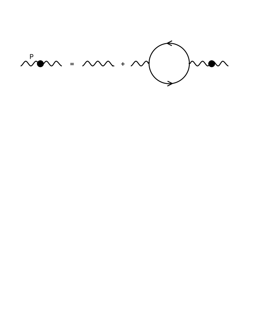
FIG. 2.: Effective photon propagator

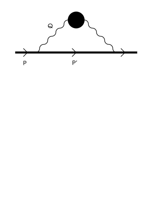
FIG. 3.: Electron self energy defining the damping rate of a hard electron

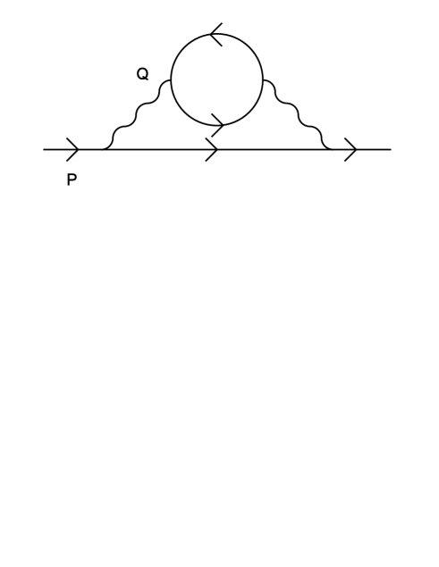
FIG. 4.: Electron self energy containing a pinch singularity

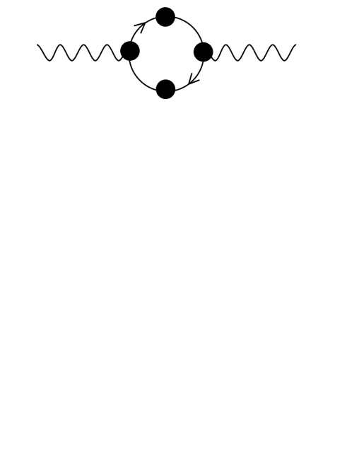
FIG. 5.: Photon self energy $\bar{\Pi}$

- [1] E. Braaten and R.D. Pisarski, Nucl. Phys. B337, 569 (1990).
- [2] M.H. Thoma, in Quark-Gluon Plasma 2, edited by R. Hwa (World Scientific, Singapore 1995), p.51.
- [3] T.S. Biró, E. van Doorn, B. Müller, M.H. Thoma, and X.N. Wang, Phys. Rev. C 48, 1275 (1993).
- [4] K. Geiger, Phys. Rep. 258, 238 (1995); X.N. Wang, Phys. Rep. 280, 287 (1997).
- [5] N.P. Landsmann and C.G. van Weert, Phys. Rep. 145, 141 (1987).
- [6] K. Chou, Z. Su, B. Hao, and L. Yu, Phys. Rep. 118, 1 (1985).
- [7] L.V. Keldysh, JETP 20, 1018 (1965).
- [8] T. Altherr and D. Seibert, Phys. Lett. B 333, 149 (1994).
- [9] M.E. Carrington and U. Heinz, Eur. Phys. J. C 1, 619 (1998).
- [10] A. Peshier, K. Schertler, and M.H. Thoma, hep-ph/9708434, Ann. Phys. (N.Y.) (in press).
- [11] H.A. Weldon, Phys. Rev. D 26, 1394 (1982); V.V. Klimov, Sov. Phys. JETP 55, 199 (1982).
- [12] R.D. Pisarski, Physica A 158, 146 (1989).
- [13] E. Braaten and M.H. Thoma, Phys. Rev. D 44, 1298 (1991).
- [14] J.P. Blaizot and E. Iancu, Phys. Rev. Lett. 76, 3080 (1996).
- [15] R. Baier, M. Dirks, K. Redlich, and D. Schiff, Phys. Rev. D 56 (1997) 2548.
- [16] M. Le Bellac and H. Mabilat, Z. Phys. C 75, 137 (1997).
- [17] P.A. Henning, Nucl. Phys. A582, 633 (1994); P.F. Bedaque, Phys. Lett. B 344, 23 (1995); C. Greiner and S. Leupold, hep-ph/9802312 and hep-ph/9804239.
- [18] T. Altherr, Phys. Lett. B 341, 325 (1995).
- [19] E. Braaten and T.C. Yuan, Phys. Rev. Lett. 66, 2183 (1991).
- [20] M.H. Thoma, Phys. Rev. D 49, 451 (1994).
- [21] H. Defu and U. Heinz, hep-ph/9704392, Eur. Phys. J. C (in press).
- [22] M.E. Carrington, H. Defu, and M.H. Thoma, hep-ph/9801103.