STRONGLY INTERACTING VECTOR BOSONS
AT TeV $e^{\pm}e^{-}$ LINEAR COLLIDERS

ABSTRACT

In the absence of light Higgs bosons, the $W$ and $Z$ bosons become strongly interacting particles at energies of about 1 TeV. If the longitudinal $W$,$Z$ components are generated by Goldstone modes associated with spontaneous symmetry breaking in a new strong interaction theory, the quasi-elastic $W$,$Z$ scattering amplitudes can be predicted as a systematic chiral expansion in the energy. We study the potential of TeV $e^{+}e^{-}$ and $e^{-}e^{-}$ linear colliders in investigating these scattering processes. We estimate the accuracy with which the coefficients of the chiral expansion can be measured in a multi-parameter analysis. The measurements will provide us with a quantitative test of the dynamics underlying the $W$,$Z$ interactions.

1 Introduction

Elastic scattering amplitudes of massive vector bosons grow indefinitely with energy if they are calculated as a perturbative expansion in the coupling of a non-abelian gauge theory. As a result, they manifestly violate unitarity beyond a critical energy scale $\sqrt{s_{c}}$ [1]. In fact, the $S$-wave scattering amplitude of longitudinally polarized $W,Z$ bosons in the isoscalar channel $(2W^{+}W^{-}+ZZ)/\sqrt{3}$,

$$a_{0}^{0}(s)=\frac{\sqrt{2}\,G_{F}s}{16\pi}+O(g^{2},g^{\prime 2})$$ (1)

must be bounded by 1/2. Unitarity therefore is violated for energies in excess of

$$\sqrt{s_{c}}\sim 1.2\;{\rm TeV}$$ (2)

in $WW$ scattering.

This problem can be solved in two different ways. In the Standard Model [2] a novel scalar particle, the Higgs boson, is introduced to restore unitarity at high energies [3, 4]. The additional contribution due to the exchange of this particle in the scattering amplitude of longitudinal vector bosons cancels the asymptotic rise of the Yang-Mills amplitude if the coupling of the Higgs particle to the $W,Z$ bosons is chosen properly. In that case, the tree-level amplitude approaches a constant value. Electroweak observables in the fermion/gauge boson sector of the Standard Model are affected by radiative corrections which depend logarithmically on the Higgs boson mass $M_{H}$. From the high-precision data at LEP1, SLC, and the Tevatron, an upper limit of $M_{H}<550\;{\rm GeV}$ has been derived at the $2\sigma$ level [5]. This limit is not sharp: Excluding one or two observables from the analysis weakens the bound significantly [6]. In a cautious conclusion the experimental limit may therefore be interpreted within the minimal model as indicative for a scale $<O(1\;{\rm TeV})$.

However, there exists a second solution to the unitarity problem. If the Higgs boson is not realized in Nature, the $W$ bosons become strongly interacting particles at TeV energies. In such a scenario the experimental upper bound of $\sim 1\;{\rm TeV}$ can be re-interpreted as the cut-off scale up to which the Standard Model of fermions and vector bosons may be extended before new physical phenomena become apparent. Such novel strong interactions of the $W$ bosons may be indicated by slight deviations of the static electroweak $W,Z$ parameters from the predictions in the Standard Model, i.e., for the oblique parameters, the $Z$-fermion couplings, the magnetic dipole, and the electric quadrupole moments of the $W^{\pm}$ bosons [7, 8, 9]. However, besides the production of triple gauge bosons in $e^{+}e^{-}$ annihilation [10], the classical test ground for these interactions is the elastic and quasi-elastic $2\to 2$ scattering experiments of the $W^{\pm}$ and $Z$ bosons

$$WW\to WW$$ (3)

where $W$ generically denotes the particles $W^{\pm},Z$.

It is natural, though not compulsory, to trace back the strong interactions of the $W$ bosons to a new fundamental strong interaction characterized by a scale of order $1\;{\rm TeV}$ [11]. If the Lagrangean of the underlying theory is globally chiral-invariant, this symmetry may be broken spontaneously. The Goldstone bosons associated with the spontaneous symmetry breaking can be absorbed by the gauge bosons to generate the masses and to build up their longitudinal degrees of freedom. It may be assumed in this scenario that the breaking pattern of the chiral symmetry in the strongly interacting sector is such that $SU(2)\times SU(2)\to SU(2)_{c}$ leaves the isospin group $SU(2)_{c}$ unbroken. This custodial $SU(2)_{c}$ symmetry [11] automatically ensures that the $\rho$ parameter, the ratio of the neutral-current to charged-current couplings, is unity up to small perturbative corrections. This condition [12] is strongly supported by the electroweak precision data. The fact that in such a scenario the longitudinally polarized $W$ bosons are associated with the Goldstone modes of chiral symmetry breaking, has far-reaching consequences which are formalized in the Equivalence Theorem [4, 13, 14, 15]. This mechanism can be exploited to predict the scattering amplitudes of the $W_{L}$ bosons for high energies below the mass scale of new resonances. Expanding the scattering amplitudes in powers of the energy $\sqrt{s}$, the leading term is parameter-free, thus being a consequence per se of the chiral symmetry breaking mechanism, independent of the particular dynamical theory. The higher-order terms in the chiral expansion depend on new coefficients which reflect the detailed structure of the underlying strong-interaction theory. With rising energy they may evolve towards a resonant behavior, in the scalar or vector channels for instance.

To study potentially strong interactions between $W$ bosons requires energies in the TeV range. They will be provided by the $pp$ collider LHC and by future $e^{+}e^{-}$ linear colliders which will operate in the second phase at energies of $1.5$ to $2\;{\rm TeV}$, see e.g. Ref.[16]. Longitudinal $W$ bosons are radiated off quarks and electrons/positrons with a probability $g^{2}/16\pi^{2}\sim 3\times 10^{-3}$; since the $Z$ charge of leptons is small, the radiation of $Z$ bosons is suppressed compared to $W$ bosons. The following (quasi-)elastic processes can be studied in $e^{+}e^{-}$ and $e^{-}e^{-}$ collisions [17, 18, 19]:

$$\begin{array}[]{l@{\quad\to\quad}l@{\quad:\quad}l@{\quad\to\quad}l}e^{+}e^{-}&\bar{\nu}_{e}\nu_{e}W^{+}W^{-}&W^{+}W^{-}&W^{+}W^{-}\\ e^{+}e^{-}&\bar{\nu}_{e}\nu_{e}ZZ&W^{+}W^{-}&ZZ\\ e^{-}e^{-}&\nu_{e}\nu_{e}W^{-}W^{-}&W^{-}W^{-}&W^{-}W^{-}\end{array}$$ (4)

It turns out that the rates for these processes are sufficiently large for thorough analyses at $e^{+}e^{-}$ c.m. energies of $\sqrt{s}\sim 1\;{\rm TeV}$ and above. Other processes involving initial state $Z$ bosons,

$$\begin{array}[]{l@{\quad\to\quad}l@{\quad:\quad}l@{\quad\to\quad}l}e^{+}e^{-}&\bar{\nu}_{e}e^{-}W^{+}Z&W^{+}Z&W^{+}Z\\ e^{+}e^{-}&e^{+}e^{-}ZZ&ZZ&ZZ\end{array}$$ (5)

are suppressed for the reasons discussed above. Nevertheless, they must be investigated to achieve a complete determination of the quartic gauge interactions in next-to-leading order of the chiral expansion. Since all basic scattering processes (4) and (5) lead to different final states, they can be disentangled in principle [though this may not be so straightforward in practice since the final state electrons and positrons may be lost in the forward directions].

The main objective of the present analysis are theoretical predictions for the processes (4) and (5) in the region where the $W,Z$ bosons become strongly interacting but the energies do not reach yet the resonance region, which may be delayed until a scale of $4\pi v\sim 3\;{\rm TeV}$ is approached. We study the predictions in leading order of the chiral expansion and analyze the sensitivity to next-to-leading order contributions. This will enable us to estimate the accuracy with which the parameter-free leading-order amplitudes can be measured. If the Higgs mechanism is not realized in Nature, these analyses will shed light on the symmetry structure and the basic physical mechanism that provides masses to the fundamental electroweak bosons. Alternative approaches that are not based on chiral symmetry breaking, would in general lead to quite different predictions for $WW$ scattering amplitudes.

The paper is organized as follows. In Sec.2 we briefly recapitulate the basic formalism of electroweak chiral Lagrangeans. In Sec.3 the helicity amplitudes for the $WW\to WW$ fusion signals are analyzed, while Sec.4 is devoted to the equivalent particle approximations and kinematical improvements. This discussion serves as a useful guideline for the analysis and as an independent check for the complete $f_{1}f_{2}\rightarrow{f^{\prime}}_{1}{f^{\prime}}_{2}WW$ tree-level calculations. The full calculation and the results for probing both the custodial $SU(2)_{c}$ conserving and breaking chiral parameters at TeV $e^{\pm}e^{-}$ linear colliders are presented in Sec.5 and 6. Conclusions are given in Sec.7. In Appendices A and B, constraints from unitarity bounds are derived and the leading contributions of the one-loop radiative corrections are estimated. The exact tree-level $WW\to WW$ helicity amplitudes are summarized in compact form up to next-to-leading order in Appendix C.

2 Chiral Lagrangeans

For theories in which the chiral symmetry is broken spontaneously, i.e., $SU(2)\times SU(2)\to SU(2)_{c}$, effective Lagrangeans can be defined for the associated Goldstone fields. They correspond to expansions in the dimensions of the field operators, or equivalently in the energy $\sqrt{s}$ in momentum space [21, 22]. This systematic expansion leads to a parameter-free leading-order interaction in the Lagrangean, supplemented by higher-order terms which reflect the detailed structure of the underlying strong interaction theory. Thus the leading-order interaction is a direct model-independent consequence of chiral symmetry breaking sui generis. The Equivalence Theorem then allows to re-interpret scattering amplitudes derived for the Goldstone particles as equivalent to the scattering amplitudes of the longitudinally polarized $W,Z$ particles for asymptotic energies $E(W,Z)\gg M_{W,Z}$.

The kinetic terms of the gauge fields and the first terms in the chiral Lagrangean of the Goldstone fields are given by the following expansion:

$${\cal L} = {\cal L}_{g}+{\cal L}_{e}$$ (6)

$${}+{\cal L}_{0}+{\cal L}_{4}+{\cal L}_{5}+\ldots$$

${\cal L}_{g}$ denotes the kinetic terms of the $W^{\pm,3}$ and $B$ fields. The $SU(2)\times U(1)$ gauge fields are coupled to the matter fields through covariant derivatives in ${\cal L}_{e}$. These two parts of the Lagrangean are given by the expressions

$${\cal L}_{g} = -\textstyle\frac{1}{8}{\rm tr}[W_{\mu\nu}^{2}]-\textstyle\frac{1}{4}B_{\mu\nu}^{2}$$ (7)

$${\cal L}_{e} = \bar{e}_{\rm L}iD\!\!\!\!/\,\,e_{\rm L}+({\rm L}\leftrightarrow{\rm R})$$ (8)

with the usual definition of the covariant $SU(2)\times U(1)$ derivative in terms of the vector fields, the $SU(2)$ generators $T^{a}$, and the hypercharge $Y$:

$$iD_{\mu}=i\partial_{\mu}+g\vec{T}\cdot\vec{W}_{\mu}-g^{\prime}{Y\over 2}B_{\mu}$$ (9)

where $2{\vec{T}}$ is equal to the Pauli matrix $\vec{\tau}$. In the general $R_{\xi}$ gauge the Goldstone fields are described by the unitary matrix

$$U=\exp[-i{\vec{w}}\cdot{\vec{\tau}}/F]$$ (10)

The custodial-symmetric dimension-2 operator of the Goldstone fields is then given by

$${\cal L}_{0}=\textstyle\frac{F^{2}}{4}{\rm tr}[D_{\mu}U^{\dagger}D^{\mu}U]$$ (11)

The coupling between the Goldstone particles and the $W$, $B$ gauge fields is parameterized by the coefficient $F$. The value of this parameter is fixed by the measured $W$ or $Z$ masses,

$${\cal L}_{0}=M_{W}^{2}W^{+}W^{-}+\frac{1}{2}M_{Z}^{2}Z^{2}+\ldots$$ (12)

so that the experimental value

$$F=(\sqrt{2}\,G_{F})^{-1/2}=246\;{\rm GeV}$$ (13)

can be derived for $F$ from the Fermi constant. In the Standard Model, $F$ is replaced by the expectation value $v$ of the Higgs field in the ground state, $F=v$. However, the physical interpretation of these parameters is completely different in the two scenarios.

A vector field $V_{\mu}$ can be defined by the Goldstone fields as

$$V_{\mu}=U^{\dagger}D_{\mu}U$$ (14)

corresponding to the derivative $\partial_{\mu}\vec{w}+\ldots$ for small field strengths. From the vector field two independent dimension-4 operators may be formed

$${\cal L}_{4} = \alpha_{4}\,{\rm tr}\left[V_{\mu}V_{\nu}\right]\,{\rm tr}\left[V^{\mu}V^{\nu}\right]$$ (15)

$${\cal L}_{5} = \alpha_{5}\,{\rm tr}\left[V_{\mu}V^{\mu}\right]\,{\rm tr}\left[V_{\nu}V^{\nu}\right]$$ (16)

which describe the first two non-leading and model-dependent terms in the chiral expansion. The two interaction terms ${\cal L}_{4}$ and ${\cal L}_{5}$ are custodial symmetric, leaving the value $\rho=1$ unchanged. Since they involve at least a quartic coupling of the Goldstone particles, they affect in lowest order only $2\to 2$ scattering processes but do not affect the trilinear vertices. Thus, $\alpha_{4}$ and $\alpha_{5}$ can only be determined in $WW\to WW$ scattering. [Additional dimension-4 operators affect the trilinear couplings; in this analysis they are assumed to be pre-determined by standard methods such as $WW$ pair production in $e^{+}e^{-}$ annihilation.]

We assume that all higher-order coefficients in the chiral expansion are much smaller than unity. Even though a gauge-symmetric chiral Lagrangean can be defined formally for any theory with a particular particle content, this is meaningful only if the chiral series can be truncated at a fixed operator dimension ($d=4$ for our purpose) and still higher orders can be neglected. However, if the concept of spontaneous chiral symmetry breaking were not realized in Nature, higher-order coefficients would be so large that an infinite number of terms would enter even at the $W,Z$ mass scale. In that case, the above effective-theory formalism must be abandoned.

From the magnitude of loop effects which carry a factor $1/16\pi^{2}$ together with an additional power of $s/v^{2}$, the largest value of $\sqrt{s}$ for a chiral expansion to be valid may be estimated [23] as $\sqrt{s}\lesssim 4\pi v\sim 3\;{\rm TeV}$. Thus, if the coefficients $\alpha_{i}$ in the chiral expansion were experimentally required to be substantially larger than $1/16\pi^{2}$, new resonance effects would already appear below the $3\;{\rm TeV}$ scale, e.g., thresholds for resonance production would become visible in the intermediate range between about $1$ and $3\;{\rm TeV}$.

Although the ’t Hooft-Feynman gauge turns out to be most convenient for the computation method described below (Sec.5), all observable quantities can be calculated equally well within the unitary gauge in which the Goldstone fields $\vec{w}$ are set to zero. In this gauge the physical content of the various terms becomes more transparent: The standard vector boson interactions are determined by the Yang-Mills kinetic Lagrangean alone, ${\cal L}_{0}$ just provides the $W,Z$ masses, and the new dimension-4 operators ${\cal L}_{4,5}$ are recognized as two independent contact-interaction terms for the $W,Z$ vector bosons:

$${\cal L}_{0} = M_{W}^{2}W^{+}_{\mu}{W^{-}}^{\mu}+\frac{1}{2}M_{Z}^{2}Z_{\mu}Z^{\mu}$$ (17)

$${\cal L}_{4} = \alpha_{4}\left[\frac{g^{4}}{2}\left[(W^{+}_{\mu}{W^{-}}^{\mu})^{2}+(W^{+}_{\mu}{W^{+}}^{\mu})(W^{-}_{\nu}{W^{-}}^{\nu})\right]\right.$$ (18)

$${}\left.+\frac{g^{4}}{c_{w}^{2}}(W^{+}_{\mu}Z^{\mu})(W^{-}_{\nu}Z^{\nu})+\frac{g^{4}}{4c_{w}^{4}}(Z_{\mu}Z^{\mu})^{2}\right]$$

$${\cal L}_{5} = \alpha_{5}\left[{g^{4}}(W^{+}_{\mu}{W^{-}}^{\mu})^{2}+\frac{g^{4}}{c_{w}^{2}}(W^{+}_{\mu}{W^{-}}^{\mu})(Z_{\nu}Z^{\nu})+\frac{g^{4}}{4c_{w}^{4}}(Z_{\mu}Z^{\mu})^{2}\right]$$ (19)

[$c_{w}^{2}=1-\sin^{2}\theta_{w}$ and $g^{2}=e^{2}/\sin^{2}\theta_{w}$]. The contact terms introduce all possible quartic couplings $W^{+}W^{-}W^{+}W^{-}$, $W^{+}W^{-}ZZ$, and $ZZZZ$ among the weak gauge bosons, that are compatible with charge conservation and custodial $SU(2)_{c}$ symmetry.

3 $WW$ scattering

From the effective chiral Lagrangean, the $2\to 2$ (quasi-)elastic $WW$ scattering amplitudes can easily be derived. As shown generically in Fig.1, they involve $s$-channel, $t/u$-channel exchange diagrams, and the non-abelian quartic boson coupling, with their sum growing asymptotically proportional to $s$. The additional quartic contributions introduced by ${\cal L}_{4}$ and ${\cal L}_{5}$ rise proportional to $s^{2}$. The maximal power of $s$ is realized only for amplitudes in which all four vector bosons are longitudinally polarized; replacing any longitudinally polarized external particle by a transversely polarized particle removes one factor of $\sqrt{s}/v$; at the same time an additional power of the weak couplings $g,g^{\prime}$ is introduced. [In the extreme forward and backward directions where $t,u$ are of the order $M_{W,Z}^{2}$, the power counting is invalid and both longitudinal and transversal degrees of freedom contribute with comparable magnitude.]

Figure 1: Feynman graphs for (quasi-)elastic $WW$ scattering.

It follows [1, 13] from analyticity, crossing symmetry, CP invariance, and custodial symmetry, that to leading order in the Yang-Mills couplings all (quasi-)elastic amplitudes can be expressed in terms of a single function $A(s,t,u)$ which is symmetric with respect to the exchange $(t\leftrightarrow u)$. This function is analytic in the Mandelstam variables $s,t,u$ apart from the usual one-particle pole and two-particle cut singularities. The Mandelstam variables are given by the total energy and the momentum transfer in the scattering processes: $s=E_{c.m.}^{2}$, $t(u)\approx-s(1\mp\cos\theta)/2$ for $|s|,|t|,|u|\gg M_{W}^{2}$. The amplitudes of the scattering processes (4) and (5) can be derived from the master amplitude $A$ in the following way:

$$A(W^{+}W^{-}\to ZZ) = A(s,t,u)$$ (20)

$$A(W^{+}W^{-}\to W^{+}W^{-}) = A(s,t,u)+A(t,s,u)$$ (21)

$$A(W^{-}W^{-}\to W^{-}W^{-}) = A(t,s,u)+A(u,t,s)$$ (22)

and

$$A(W^{+}Z\to W^{+}Z) = A(t,s,u)$$ (23)

$$A(ZZ\to ZZ) = A(s,t,u)+A(t,s,u)+A(u,t,s)$$ (24)

To leading order in the energy expansion the amplitude $A(s,t,u)$ is reduced to the simple expression

$$A(s,t,u)_{\rm LO}=\frac{s}{v^{2}}$$ (25)

which is parameter-free. The next-to-leading order terms modify this result, and the final tree-level expression is given to order $s^{2}$ by

$$A(s,t,u)=\frac{s}{v^{2}}+\alpha_{4}\frac{4(t^{2}+u^{2})}{v^{4}}+\alpha_{5}\frac{8s^{2}}{v^{4}}$$ (26)

The relations (20–24) for the amplitudes are preserved by loop corrections and they are valid to all orders for chirally-symmetric strong interactions. There are, however, additional perturbative corrections which are proportional to the Yang-Mills couplings $g,g^{\prime}$, with the $g^{\prime}$ coupling breaking the custodial symmetry. Amplitudes involving transversely polarized vector bosons, which are subleading both for high energies and in the weak coupling expansion, do not respect the relations (20–24).

It is instructive to analyze the angular momentum states that are populated in $WW$ scattering. The helicity analysis [24] of the scattering amplitudes leads to the following decomposition in the angular momentum

$$A(00,00)=\sum_{J}A_{J}(00,00)\;d_{00}^{J}(\theta)$$ (27)

for longitudinally polarized vector bosons, where $d_{00}^{J}=P_{J}(\cos\theta)$ are the Legendre Polynomials.

Choosing the process $W^{+}W^{-}\to ZZ$ for example, the gauge contributions to the amplitudes involve $t$- and $u$-channel exchange diagrams, giving rise to arbitrarily high orbital angular momentum states. Therefore we decompose the amplitude with respect to spin only, i.e., the residues of the poles for $t/u$-channel diagrams are expanded:

$$A_{J}=\displaystyle\frac{s^{2}}{4M_{W}^{4}}\left[{g^{2}c_{w}^{4}}\left(\frac{s}{2(t-M_{W}^{2})}\hat{A}_{t}+\frac{s}{2(u-M_{W}^{2})}\hat{A}_{u}+\hat{A}_{c}\right)+g^{4}\left(\alpha_{4}\hat{A}_{4}+\alpha_{5}\hat{A}_{5}\right)\right]$$ (28)

The subscripts $t,u,c$ for $\hat{A}$ denote the $t,u$ exchange and the four-boson contact terms, respectively (Tab.1).

$$\begin{array}[]{|r|rrr|cc|}\hline\cr&\hat{A}_{t}&\hat{A}_{u}&\hat{A}_{c}&\hat{A}_{4}&\hat{A}_{5}\rule[-5.0pt]{0.0pt}{18.0pt}\\ \hline\cr J=0&-\frac{20}{3}&-\frac{20}{3}&-\frac{16}{3}&\frac{8}{3}&8\rule[-5.0pt]{0.0pt}{18.0pt}\\ 1&\frac{44}{5}&-\frac{44}{5}&0&0&0\rule[-5.0pt]{0.0pt}{18.0pt}\\ 2&-\frac{4}{3}&-\frac{4}{3}&\frac{4}{3}&\frac{4}{3}&0\rule[-5.0pt]{0.0pt}{18.0pt}\\ 3&-\frac{4}{5}&\frac{4}{5}&0&0&0\rule[-5.0pt]{0.0pt}{18.0pt}\\ \hline\cr\end{array}$$

Table 1: Amplitude decomposition for the process $W^{+}W^{-}\to ZZ$ in the limit $E\gg M_{W}$.

In the spin amplitudes, the contact term contains angular momenta $J=0$ and $2$. In the $t/u$ channel diagrams the additional vector boson in the intermediate state populates, together with the external vector bosons, the states up to $J=3$. In the limit $|s|,|t|,|u|\gg M_{W}^{2}$ the leading $s^{2}$ behavior cancels for $\alpha_{4}=\alpha_{5}=0$; however, in the forward/backward regions ($|t|,|u|\sim M_{W}^{2}$) this cancellation needs not occur. In other processes such as $W^{+}W^{-}\to W^{+}W^{-}$ there is an additional $s$-channel diagram which is purely spin-1, since a single vector boson $Z/\gamma$ is exchanged.

Given the helicity amplitudes, the differential cross sections can be written as

$$\frac{d\sigma}{d\cos\theta}(W_{\lambda_{1}}W_{\lambda_{2}}\to W_{\lambda_{3}}W_{\lambda_{4}})=\frac{1}{32\pi s}\left|A(\lambda_{1}\lambda_{2},\lambda_{3}\lambda_{4})\right|^{2}~{}.$$ (29)

This cross section can easily be integrated over all angles,

$$\sigma(W_{\lambda_{1}}W_{\lambda_{2}}\to W_{\lambda_{3}}W_{\lambda_{4}})=\frac{\eta}{32\pi s}\int_{-1}^{1}d(\cos\theta)\left|A(\lambda_{1}\lambda_{2},\lambda_{3}\lambda_{4})\right|^{2}$$ (30)

where $\eta=\frac{1}{2}(1)$ accounts for (non-)identical particles in the final state.

Even though the longitudinal helicities build up the asymptotically leading cross section $\sigma(W_{L}W_{L}\to W_{L}W_{L})$, it cannot be identified with the total cross section without applying angular cuts for non-asymptotic energies since the forward peak for the scattering of transversely polarized $W$ bosons gives rise to additional large contributions to the total cross section.

Interference effects between different helicity amplitudes in the initial state have to be taken into account in the non-asymptotic regime. Since the $W$ bosons are radiated off the electrons and positrons, a coherent mixture of $W_{\lambda_{1}}W_{\lambda_{2}}$ helicity states is generated with $\lambda_{1}$ and $\lambda_{2}=\pm,0$. Interference effects in the final $W_{\lambda_{3}}W_{\lambda_{4}}$ state need only to be included if the angular and energy distributions of the leptons or jets in the $W_{3},W_{4}$ decays are analyzed explicitly.

4 Equivalent particle approximations

The elastic scattering of $W$ bosons at high energies will be studied in TeV $e^{+}e^{-}$ and $e^{-}e^{-}$ collisions. At high energies electron/positron beams split for a long time into (neutrino $+W$) or (electron/positron $+Z$) pairs. In fact, if the transverse momentum in the splitting process is $p_{\perp}$, the lifetime of the split state is of order $\tau\sim E_{e}/(p_{\perp}^{2}+M_{W}^{2})$ in the laboratory, which is large for high electron/positron energies. With $E_{e}=800\;{\rm GeV}$ the lifetime $\tau\sim 10^{-1}\;{\rm GeV}^{-1}$ is an order of magnitude longer than the weak interaction scale $\tau_{w}\sim M_{W}^{-1}\sim 10^{-2}\;{\rm GeV}^{-1}$. The $W$ bosons can therefore be approximately treated as equivalent particles [25], similar to the equivalent photon approximation in QED [26]. Moreover, the splitting probability is maximal for small transverse momenta $p_{\perp}\lesssim M_{W}$. In the final picture, the $W$ bosons can be treated as real particle beams which accompany the parent $e^{\pm}$ beams in the accelerator.

The energy spectrum of the $W$ bosons can conveniently be determined, in the spirit of the discussion above, by old-fashioned perturbation theory [27]. Denoting the fraction of energy transferred from the initial lepton to the $W$ boson by $x$, with $0\leq x\leq 1$, the spectra, under the leading logarithmic approximation, are given by [25]:

1. Transversely polarized $W^{\pm}$ bosons:

   $$f^{T}_{W/e}(x) = \frac{\alpha}{4\pi s_{w}^{2}}\,\frac{1+(1-x)^{2}}{2x}\ln\frac{\hat{s}}{M_{W}^{2}}$$ (31)

   where $\hat{s}=xs$.

   For $e^{-}$ beams, the term $\sim 1$ corresponds to negative helicity of the $W$ boson, while the term $\sim(1-x)^{2}$ corresponds to positive helicity, suppressed for $x\to 1$ by the conservation of angular momentum. [The role of the helicities is interchanged for $e^{+}$ beams.] The spectrum increases with the logarithm of the energy, which is a consequence of the unlimited transverse momentum of the point-like coupling in the splitting process.

2. Longitudinally polarized $W^{\pm}$ bosons:

   $$f^{L}_{W/e}(x) = \frac{\alpha}{4\pi s_{w}^{2}}\,\frac{1-x}{x}$$ (32)

   Since the emission of longitudinally polarized $W$ bosons is suppressed for large transverse momentum, the longitudinal spectra are not logarithmically enhanced.

In the equivalent particle approximation the cross section $d\sigma$ for the colliding beam process, such as

$$e^{+}e^{-}\to\bar{\nu}_{e}\nu_{e}W^{+}W^{-}\qquad\mbox{via}\qquad W^{+}W^{-}\to W^{+}W^{-}$$ (33)

can be obtained by convoluting the cross section $d\hat{\sigma}$ of the $WW$ subprocess with the spectra of the two initial-state $W$ bosons:

$$d\sigma[e^{+}e^{-}\to\bar{\nu}_{e}\nu_{e}W^{+}W^{-}]$$ (34)

$$= \int_{0}^{1}dx_{1}\int_{0}^{1}dx_{2}\,f_{W/e}(x_{1})f_{W/e}(x_{2})\,d\hat{\sigma}[W^{+}W^{-}\to W^{+}W^{-};\hat{s}=x_{1}x_{2}s]$$

The c.m. invariant energy of the subprocess is given by $\sqrt{\hat{s}}=\sqrt{x_{1}x_{2}s}$. The fixing of final-state observables $\Omega$ can be implemented by restricting the integration over the phase space $\hat{\Phi}$ appropriately:

$$\frac{d\sigma}{d\Omega}[e^{+}e^{-}\to\bar{\nu}_{e}\nu_{e}W^{+}W^{-}]=\int_{0}^{1}dx_{1}\int_{0}^{1}dx_{2}\,f_{W/e}(x_{1})f_{W/e}(x_{2})\,\frac{d\hat{\sigma}}{d\hat{\Phi}}d\hat{\Phi}\,\delta\left(\Omega-\Omega(x_{1},x_{2})\right)$$ (35)

Other $W,Z$ processes can be treated analogously.

The commonly used equivalent particle spectra in the leading logarithmic approximation, Eqs.(31)-(32), are derived in the small-angle limit with zero $p_{\perp}$. To suppress background processes which are induced by Weizsäcker-Williams photons, it is necessary to consider the transverse momentum distribution of the $W$ boson pair. To high accuracy, the c.m. frame of $\gamma$-initiated subprocesses moves parallel to the $e^{\pm}$ beams. The $W$-initiated signal processes, by contrast, have transverse momenta of order $P_{\perp}(WW)\sim M_{W}$. Hence, the $\gamma$-initiated background processes can be eliminated by cutting on the total transverse momentum of the subprocess with respect to the $e^{\pm}$ beams. For the above reason, the usual leading logarithmic equivalent-particle approximation, (31)-(32), cannot be applied when a $P_{\perp}(WW)$ cut is imposed in the analysis. In order to provide a guideline for the later more complete analysis, we start with the improved equivalent-particle formalism[29], from which we derive the $P_{\perp}(WW)$ distribution. This can be most conveniently performed by relating the $W$ transverse momentum to its virtual mass squared $q^{2}$:

$$p_{\perp}=\frac{\sqrt{s}}{2}(1-x)\sqrt{1-\left[1+\frac{2q^{2}}{s(1-x)}\right]^{2}}$$ (36)

with the space-like $q^{2}$ bounded by $-s(1-x)\leq q^{2}\leq 0$. Expressed in terms of $q^{2}$, the improved equivalent particle distributions can be written as

$$f^{\lambda}_{W/e}(x)=\frac{\alpha x}{16\pi s_{w}}\int_{q^{2}_{\min}}^{q^{2}_{\max}}\frac{-q^{2}dq^{2}}{(q^{2}-M_{W}^{2})^{2}}\left\{\begin{array}[]{ll}\displaystyle\frac{M_{W}^{2}\kappa_{1}^{2}}{-q^{2}}&\mbox{for $\lambda=L$}\\[12.80365pt] \displaystyle(1+\kappa_{2}^{2})&\mbox{for $\lambda=T$}\end{array}\right.$$ (37)

where

$$\kappa_{1}\equiv\frac{2\sqrt{1-x+q^{2}/s}}{x-q^{2}/s}\qquad\kappa_{2}\equiv\frac{2}{x-q^{2}/s}-1$$ (38)

and $\lambda=L,T$ denotes longitudinal resp. transverse polarization. In the latter case we have added the results for negative and positive helicity of the $W$ boson.

The improved luminosity distributions of the $W$ bosons with respect to the transverse momentum are thus given as follows:

$$f^{\lambda}_{W/e}(x,p_{\perp}^{2})=\frac{\alpha}{4\pi s_{w}^{2}}\left\{\begin{array}[]{ll}\displaystyle\frac{\kappa_{m}x\kappa_{1}^{2}}{s\bar{x}r(\bar{x}\bar{r}+2\kappa_{m})^{2}}&~{}~{}~{}~{}\mbox{for $\lambda=L$}\\[12.80365pt] \displaystyle\frac{x\bar{r}(1+\kappa_{2}^{2})}{2sr(\bar{x}\bar{r}+2\kappa_{m})^{2}}&~{}~{}~{}~{}\mbox{for $\lambda=T$}\end{array}\right.$$ (39)

with

$$\kappa_{\perp}\equiv\frac{{p_{\perp}}^{2}}{s}\qquad\kappa_{m}\equiv\frac{M_{W}^{2}}{s}\qquad r\equiv\sqrt{1-\frac{4\kappa_{\perp}}{(1-x)^{2}}}\qquad\bar{x}\equiv 1-x\qquad\bar{r}\equiv 1-r$$ (40)

In the asymptotic limit $s\gg P_{\perp}^{2},M_{W}^{2}$, and for $x_{1,2}$ neither close to 0 nor 1, we can derive the following approximate formula from eq.(39):

$$f^{T}_{W/e}(x,p_{\perp}^{2}) = \frac{\alpha}{4\pi s_{w}^{2}}\,\frac{1+(1-x)^{2}}{2x}\,\frac{p_{\perp}^{2}}{\left(p_{\perp}^{2}+(1-x)M_{W}^{2}\right)^{2}}$$ (41)

$$f^{L}_{W/e}(x,p_{\perp}^{2}) = \frac{\alpha}{4\pi s_{w}^{2}}\,\frac{1-x}{x}\,\frac{(1-x)M_{W}^{2}}{\left(p_{\perp}^{2}+(1-x)M_{W}^{2}\right)^{2}}$$ (42)

The transverse momentum distribution ($~{}f^{\lambda_{1}\lambda_{2}}_{WW/ee}(x,P_{\perp}^{2};\hat{s})~{}$) of the two-particle $WW$ system can be approximately derived by convoluting the spectra (39) for each initial $W$ boson:

$$\displaystyle d\sigma(e+e\rightarrow f_{3}+f_{4}+X\mid s)=\sum_{\lambda}\int_{0}^{1}dx\int dP_{\perp}^{2}f^{\lambda_{1}\lambda_{2}}_{WW/ee}(x,P_{\perp}^{2};\hat{s})d\widehat{\sigma}(W_{\lambda_{1}}+W_{\lambda_{2}}\rightarrow X\mid\hat{s})$$ (43)

$$f^{\lambda_{1}\lambda_{2}}_{WW/ee}(x,P_{\perp}^{2};\hat{s})=\int_{x}^{1}\!\int_{0}^{1}dx_{1}dx_{2}\int\!\!\!\int d{p}_{1\perp}^{2}d{p}_{2\perp}^{2}D(x)\,D(P_{\perp}^{2})\,f^{\lambda_{1}}_{W/e}(x_{1},p_{1\perp}^{2})\,f^{\lambda_{2}}_{W/e}(x_{2},p_{2\perp}^{2})$$ (44)

with

$$D(x) = \delta(x-x_{1}x_{2})|_{\hat{s}=xs}$$ (45)

$$D(P_{\perp}^{2}) = \int_{0}^{2\pi}\frac{d\varphi_{12}}{2\pi}\,\delta({P}_{\perp}^{2}-|\vec{p}_{1\perp}+\vec{p}_{2\perp}|^{2})$$ (46)

where $\varphi_{12}$ is the azimuthal angle between the two initial $W$ bosons in the $e^{+}e^{-}$ c.m. frame. Due to the implicit $\varphi_{12}$-dependence in the squared transverse momentum, $|\vec{p}_{1\perp}+\vec{p}_{2\perp}|^{2}$, the integral in (46) is non-trivial.

Figure 2: Distribution of the $WW$ transverse momentum $P_{\perp}(WW)$ in $1.6\;{\rm TeV}$ $e^{\pm}e^{-}$ collisions.

The characteristic features of the luminosity spectra with respect to the transverse momentum of the $WW$ system are exemplified in Fig.2. In Fig.2(a) we depict the $P_{\perp}(WW)$ distributions for $x_{1}=x_{2}=0.5$. The probability for the emission of longitudinal $W$ bosons is maximal around low values of $P_{\perp}\sim M_{W}/2$ and falls off rapidly with increasing transverse momentum. The spectrum of the transverse $W$ bosons extends to much larger values of $P_{\perp}$, decreasing asymptotically like $(1/P_{\perp}^{2})\ln(M_{W}^{2}/P_{\perp}^{2})$. The $\gamma\gamma$ spectrum, by contrast, is strongly peaked at zero transverse momentum.

Since the phase space in (44) is restricted for a finite collider energy $\sqrt{s}$, the improved distributions (39) [solid lines in Fig.2(a)] decrease for large transverse momenta faster than the approximate distributions (41-42) [dotted].

In Fig.2(b) the $WW$ transverse momentum distributions (44) are depicted for two values of the invariant $WW$ mass, $M_{WW}=0.8$ and $1\;{\rm TeV}$, at a fixed collider energy of $\sqrt{s}=1.6\;{\rm TeV}$. A typical cut of $50\;{\rm GeV}$, which will be introduced below (cf. Sec.5), is indicated by the dotted line. The distributions are not shown for transverse momenta beyond $\sim 250\;{\rm GeV}$ since interference effects between the amplitudes become significant for large transverse momenta, invalidating the probabilistic picture of the single-particle distributions.

As shown in Fig.2(b), for higher values of $M_{WW}$ the distributions are shifted towards lower values of $P_{\perp}^{2}$. For a fixed $M_{WW}$, the improved $P_{\perp}$ distributions are lower than the approximate ones, as shown in Fig.2(a). For this reason, the leading logarithmic approximation generally overestimates the production rates due to transverse $W$ boson fusion by a factor of $3\sim 5$ [30, 31]. Therefore, we use the improved equivalent-particle method, in contrast to the leading logarithmic approximation, as a guideline for the analysis and as an independent check for the complete tree-level calculation. It turns out that the $\pm 1\sigma$ exclusion contours for $\alpha_{4-10}$, as shown in Figs.9, 10 and 11, obtained from the above two methods, are in good agreement after imposing all the relevant kinematic cuts to enhance the ratio of signal to background. Hence, we shall not discuss in detail the numerical results obtained by applying the equivalent-particle method, but we will focus on the improved results which are based on the exact tree-level calculations.

5 Calculation and results: Conserved custodial $SU(2)_{c}$

For a detailed numerical study, based on a complete tree-level calculation, we have chosen the three processes

$$e^{+}e^{-} \to \bar{\nu}_{e}\nu_{e}W^{+}W^{-}$$ (47)

$$e^{+}e^{-} \to \bar{\nu}_{e}\nu_{e}ZZ$$ (48)

$$e^{-}e^{-} \to \nu_{e}\nu_{e}W^{-}W^{-}$$ (49)

where the (quasi-)elastic $WW$ scattering signal corresponds to the generic diagrams depicted in Fig.3. However, there are also Feynman diagrams contributing to (47–49) which do not contain $WW$ scattering as a subprocess (cf. Fig.4). This irreducible background is not negligible and must be taken into account in the analysis.

In all signal processes there are already two neutrinos present in the final state, therefore important kinematic information is lost if a $W$ boson decays leptonically (or a $Z$ boson into two neutrinos). In particular, the c.m. energy of the subprocess cannot be determined in that case. For the present study we therefore restrict ourselves to hadronic $W,Z$ decays and to decays of the $Z$ boson into electrons and muons. Furthermore, an error in the dijet invariant mass is introduced by the limited energy resolution of the calorimeters, which leads to the rejection of a fraction of di-boson events and to the misidentification of $W$ vs. $Z$ bosons. Adopting the results for the net efficiencies determined in Ref.[17], we assume that in a hadronic decay a true $W,Z$ boson will be identified according to the following pattern:

$$W \to 85\%\;W,\ 10\%\;Z,\ 5\%\;\mbox{reject}$$ (50)

$$Z \to 22\%\;W,\ 74\%\;Z,\ 4\%\;\mbox{reject}$$ (51)

Thus, for example, when calculating the signal event rate in the $ZZ$ detection mode, one has to include the rates predicted by 55%, 7%, and 1% of the partonic $ZZ$, $W^{\pm}Z$ and $W^{+}W^{-}$ final states, respectively, to account for final-state misidentification. The relative weighting factors from the above three partonic final state cross sections are $55:7:1$ which is equal to $1:0.13:0.018$, as given in the last column of Tab.II. As discussed above, we only consider the hadronic decay modes of a final state $W$ boson, the corresponding decay branching ratio (BR) is $0.67$. For detecting a $Z$ boson, we include both the hadronic modes (BR=0.70) and the di-lepton modes (BR=0.067 for $e^{+}e^{-}$ and $\mu^{+}\mu^{-}$). Hence, the efficiency for detecting a $WW$, $ZZ$, and $WZ$ pair originating from a partonic $WW$, $ZZ$, and $WZ$ final state is 33.4%, 34.2%, and 33.8%, respectively. For simplicity, we take 33% as the detection efficiency for all the detection modes considered in this study.

Figure 3: Diagrams contributing to the strong $WW$ scattering signal.

Figure 4: Typical diagrams contributing to the irreducible background for the strong $WW$ scattering signal.

Figure 5: Partially reducible backgrounds to the strong $WW$ scattering signal.

Since the final state cannot be completely resolved experimentally in all cases, further background processes will play a role (cf. Fig.5). The most important background to the signal process $e^{+}e^{-}\to\bar{\nu}\nu W^{+}W^{-}$ is generated by the reaction

$$e^{+}e^{-}\to W^{+}W^{-}e^{+}e^{-}$$ (52)

which is built up primarily by the subprocess $\gamma\gamma\to W^{+}W^{-}$. In this process most of the electrons/positrons are emitted in forward direction so that they cannot be detected. A similar background is introduced by the misidentification of vector bosons in jet decays:

$$e^{+}e^{-}\to W^{\pm}Ze^{\mp}\nu$$ (53)

An irreducible background is also generated by three-boson final states,

$$e^{+}e^{-}\to W^{+}W^{-}Z$$ (54)

with the $Z$ decaying into neutrino pairs. Similar backgrounds (less dangerous for the $ZZ$ final state) exist for the other processes.

The total cross sections for the signal and background processes, including interference effects, have been computed in a complete tree-level calculation using the automatic package CompHEP [32] in which the effective Lagrangian (6) has been implemented. The results of the cross sections for the reference point $\alpha_{4}=\alpha_{5}=0$ are summarized in Tab.2.

$$\begin{array}[]{|l||r|r||c|}\hline\cr\mbox{Process}&{800}\ {\rm GeV}&{1.6}\ {\rm TeV}&\mbox{Factor}\\ \hline\cr\hline\cr W^{+}W^{-}\bar{\nu}\nu&11&56&1\\ W^{+}W^{-}e^{+}e^{-}&628&1979&1\\ W^{\pm}Ze^{\mp}\nu&39&173&0.26\\ W^{+}W^{-}(Z\to\bar{\nu}\nu)&13&11&1\\ \hline\cr\hline\cr ZZ\bar{\nu}\nu&4&26&1\\ ZZe^{+}e^{-}&2&4&1\\ W^{\pm}Ze^{\mp}\nu&39&173&0.13\\ W^{+}W^{-}e^{+}e^{-}&628&1979&0.018\\ ZZ(Z\to\bar{\nu}\nu)&0.6&0.4&1\\ \hline\cr\hline\cr W^{-}W^{-}\nu\nu&14&67&1\\ \hline\cr\end{array}$$

Table 2: Total cross sections in $\rm fb$ for various processes. Dectection efficiencies and branching ratios are not included. Including final-state misidentification, the numbers should be multiplied by the relative weighting factor given in the last column which accounts for final-state misidentification in the corresponding detection mode ($W^{+}W^{-}$, $ZZ$, or $W^{-}W^{-}$).

The background reduction is essential for isolating the strong scattering signal, as demonstrated by the numbers in Tab.2. To this purpose, we follow the strategy introduced in Ref.[17]:

1. We require $M_{\rm inv}(\bar{\nu}\nu)>200\,(150)\ {\rm GeV}$. The first number applies for $\sqrt{s}=1.6\;{\rm TeV}$, while the bracketed number for $\sqrt{s}=800\;{\rm GeV}$. This cut removes the events with neutrinos from $Z$ decay together with backgrounds from $W^{+}W^{-}$ and QCD four-jet production. The signal is not affected (cf. Fig.6).

   Figure 6: Distribution of the invariant $WW$ recoil mass distribution in the process $e^{+}e^{-}\to W^{+}W^{-}\bar{\nu}\nu$ (signal). The cut (shaded area) removes events in which the neutrinos are generated through $Z$ decays. The other cuts have been applied as described in the text.

2. Selecting central events [$|\cos\theta(W/Z)|<0.8$] with $p_{\perp}(W/Z)>200\,(100)\ {\rm GeV}$ removes events dominated by $t$-channel exchange in the subprocess.

3. The background from $\gamma\gamma$ fusion is reduced by two orders of magnitude if an electron veto is applied [removing events with $\theta(e)>10^{\circ}$] and, at the same time, a minimum $p_{\perp}$ of the vector boson pair, equivalent to the fermion $p_{\perp}$, is required. We use $p_{\perp}(WW)>50\,(40)\ {\rm GeV}$ and $p_{\perp}(ZZ)>30\ {\rm GeV}$. This cut removes also about one half of the signal events. (Fig.8; cf. the discussion in Sec.4)

4. Since the impact of the strong interaction terms ${\cal L}_{4}$ and ${\cal L}_{5}$ increases with the energy of the subprocess, we use a window in $M_{\rm inv}(WW/ZZ)$ between $700\,(350)$ and $1200\,(600)\ {\rm GeV}$, Fig.8. [The bulk of events has lower invariant mass, but those are quite insensitive to the parameters of interest.]

Figure 7: Transverse momentum distribution of the $W$ pair in the process $e^{+}e^{-}\to W^{+}W^{-}\bar{\nu}\nu$ at $\sqrt{s}=1.6\;{\rm TeV}$. All cuts have been applied, but the $WW$ detection efficiency (therefore, the decay branching ratio) is not included. The solid line corresponds to the reference point $\alpha_{4}=\alpha_{5}=0$, the dashed line to $\alpha_{4}=0.005$ for comparison. The dominant backgrounds $W^{+}W^{-}e^{+}e^{-}$ (dotted) and $WZe\nu$ (dot-dashed, with $26\%$ misidentification probability) are also indicated. The shaded area is removed by the $p_{\perp}$ cut.

Figure 8: Invariant mass distribution of the $W$ pair in the process $e^{+}e^{-}\to W^{+}W^{-}\bar{\nu}\nu$. Legend as in Fig.8.

After applying those cuts, we find the numbers reported in Tab.3. If they are multiplied by the misidentification probabilities in the last column, the signal/background ratios are raised to $O(1)$.

$$\begin{array}[]{|l||r|r||c|}\hline\cr\mbox{Process}&{800}\ {\rm GeV}&{1.6}\ {\rm TeV}&\mbox{Factor}\\ \hline\cr\hline\cr W^{+}W^{-}\bar{\nu}\nu&0.41&0.71&1\\ W^{+}W^{-}e^{+}e^{-}&0.12&0.47&1\\ W^{\pm}Ze^{\mp}\nu&1.42&1.23&0.26\\ W^{+}W^{-}(Z\to\bar{\nu}\nu)&0.01&0.01&1\\ \hline\cr\hline\cr ZZ\bar{\nu}\nu&0.33&0.86&1\\ ZZe^{+}e^{-}&0.00&0.00&1\\ W^{\pm}Ze^{\mp}\nu&1.54&1.37&0.13\\ W^{+}W^{-}e^{+}e^{-}&0.51&0.93&0.018\\ ZZ(Z\to\bar{\nu}\nu)&0.00&0.00&1\\ \hline\cr\hline\cr W^{-}W^{-}\nu\nu&0.81&1.36&1\\ \hline\cr\end{array}$$

Table 3: Cross sections in $\rm fb$ as in Tab.2, but including all cuts.

In order to obtain the final event rates, the cross sections in Tab.3 have to be multiplied by the expected luminosity and $33\%$ detection efficiency [cf.(50-51); this number includes the $W/Z$ decay branching ratios].

For polarized beams with left-handed electron and right-handed positron polarizations $P_{\mp}$, the rates are modified as follows:

1. Two left-handed electron/positron couplings are involved in the signal process. The rate is therefore increased by the factor $(1+P_{+})(1+P_{-})$.

2. The dominant part of the $WZ$ background is initiated by $\gamma W$ fusion which involves only one left-handed coupling. The cross section is therefore increased by the factor $1+(P_{+}+P_{-})/2$. Since the $Z$ coupling to electrons is almost of axial-vector type, this holds approximately true also for the remainder of the $WZ$ background.

3. The $WWee$ background is not modified. [There are diagrams in which the $W$’s both originate from the same fermion line. The contribution from this kind of diagrams should increase by the factor $1+(P_{+}+P_{-})/2$; however, its net effect is not important.]

We conclude that both electron and positron polarization is essential in order to improve the signal rate as well as the signal/background ratio. In the ideal case of complete polarization, $S/B$ improves by a factor $2$ and $S/\sqrt{B}$ by a factor $3$ as far as reducible backgrounds are concerned. For the irreducible part, $S/\sqrt{B}$ increases by a factor $2$ from the rate alone.

Figure 9: Upper part: Cross section including backgrounds for the process $e^{+}e^{-}\to\bar{\nu}\nu W^{+}W^{-}$. All cuts have been applied. The shaded band is the statistical error corresponding to the expected detection efficiency and a luminosity of $\int{\cal L}=500\;{\rm fb}^{-1}$. It is assumed that the $e^{-}$($e^{+}$) beam is polarized at a degree of $100\%\;(50\%)$. Lower Part: $1\sigma$ exclusion contours for all three processes in the $\alpha_{4}/\alpha_{5}$ plane, based on the hypothesis $\alpha_{4}=\alpha_{5}=0$. All cuts have been applied and detection efficiencies are included. The closed contour curve is the 90% exclusion limit obtained by combining the $e^{+}e^{-}\to\bar{\nu}\nu W^{+}W^{-}$ and $e^{+}e^{-}\to\bar{\nu}\nu ZZ$ channels.

All numbers quoted so far were based on the values $\alpha_{4}=\alpha_{5}=0$. Ultimately we are interested in the measurement of those parameters. The result of the theoretical prediction is depicted in Fig.9. In the upper part the dependence of the cross sections on $\alpha_{4}$ and $\alpha_{5}$ is displayed for polarized beams after all cuts are applied, but no detection efficiencies included. The band, based on the hypothesis $\alpha_{4}=\alpha_{5}=0$, is determined by the $\pm 1\sigma$ statistical error in the $WW\bar{\nu}\nu$ event rate if the expected integrated luminosity of $\int{\cal L}=500\;{\rm fb}^{-1}$ and the efficiency of $33\%$ [which includes the $W/Z$ decay branching ratios] are taken into account. The lower part of the figures shows the corresponding experimental regions in the two-dimensional $[\alpha_{4},\alpha_{5}]$ plane, based on the hypothesis $\alpha_{4}=\alpha_{5}=0$. We display the ($\pm 1\sigma$) bounds for the individual channels, which can be combined to give the $90\%$ exclusion limit indicated by the closed contour curve.

6 Calculation and results: Broken custodial $SU(2)_{c}$

In addition to the interactions ${\cal L}_{4,5}$ in (15–16), three more dimension-$4$ operators ${\cal L}_{6,7,10}$ are present at next-to-leading order of the electroweak chiral Lagrangian. Since these interactions affect the quartic gauge couplings only, they also do not contribute to low-energy observables at tree level:

$${\cal L}_{6} = \alpha_{6}\,{\rm tr}\left[V_{\mu}V_{\nu}\right]{\rm tr}\left[{\cal T}V^{\mu}\right]{\rm tr}\left[{\cal T}V^{\nu}\right]$$ (55)

$${\cal L}_{7} = \alpha_{7}\,{\rm tr}\left[V_{\mu}V^{\mu}\right]{\rm tr}\left[{\cal T}V_{\nu}\right]{\rm tr}\left[{\cal T}V^{\nu}\right]$$ (56)

$${\cal L}_{10} = \alpha_{10}\,\frac{1}{2}\left({\rm tr}\left[{\cal T}V^{\mu}\right]{\rm tr}\left[{\cal T}V^{\nu}\right]\right)^{2}$$ (57)

where ${\cal T}=U\tau_{3}U^{\dagger}$. Due to the presence of ${\cal T}$, the new operators ${\cal L}_{6,7,10}$ violate the custodial $SU(2)_{c}$ symmetry in contrast to ${\cal L}_{4,5}$.

The coefficients $\alpha_{4,5}$ and $\alpha_{6,7,10}$ can be constrained only indirectly from low-energy observables, to which they contribute through one-loop diagrams at the order of $\alpha_{n}{1\over 16\pi^{2}}\sim{v^{2}\over\Lambda^{2}}{1\over 16\pi^{2}}$ [33]. Since the corresponding loop divergences must be absorbed by renormalization counterterms, it is impossible to derive precise bounds on these parameters from low-energy data. Nevertheless, rough estimates can be obtained by keeping only the leading logarithmic terms. The estimated indirect bounds on these $4$-boson couplings are summarized in the following list [34, 33]

$$\begin{array}[]{c@{\qquad}c}-25\times 10^{-3}\leq\alpha_{4}\leq 125\times 10^{-3}&-4\times 10^{-3}\leq\alpha_{6}\leq 22\times 10^{-3}\\ -63\times 10^{-3}\leq\alpha_{5}\leq 318\times 10^{-3}&-32\times 10^{-3}\leq\alpha_{7}\leq 163\times 10^{-3}\\ &-4\times 10^{-3}\leq\alpha_{10}\leq 22\times 10^{-3}\end{array}$$ (58)

which are derived at $90\%$ c.l. by setting only one new parameter nonzero at a time. Even though current bounds on the $\rho$ parameter severely constrain the possible amount of $SU(2)_{c}$ violation, the next-to-leading $SU(2)_{c}$-violating parameters $\alpha_{6,7,10}$ are still allowed in the range from $0.02$ to $0.2$ which is well above the natural value $\sim 1/16\pi^{2}\simeq 0.006$.

In this section, we focus on tests of the $SU(2)_{c}$-violating operators ${\cal L}_{6,7,10}$ in quasi-elastic $WW$ scattering. Unlike the parameters $\alpha_{4,5}$, the terms $\alpha_{6,7,10}$ signal new dynamics beyond the standard model (SM), since the SM-like Higgs sector respects $SU(2)_{c}$-symmetry and thus does not contribute to $\alpha_{6,7,10}$. The leading contribution of the quasi-elastic $WW\to WW$ scattering amplitudes is associated with longitudinal gauge bosons and can be written as follows:

$$A(W^{+}W^{-}\to W^{+}W^{-}) = -\frac{u}{v^{2}}+\frac{4(s^{2}+t^{2}+2u^{2})}{v^{4}}\alpha_{4}+\frac{8(s^{2}+t^{2})}{v^{4}}\alpha_{5}$$ (59)

$$A(W^{+}W^{-}\to ZZ) = +\frac{s}{v^{2}}+\frac{4(t^{2}+u^{2})}{v^{4}}(\alpha_{4}+\alpha_{6})+\frac{8s^{2}}{v^{4}}(\alpha_{5}+\alpha_{7})$$ (60)

$$A(W^{-}W^{-}\to W^{-}W^{-}) = -\frac{s}{v^{2}}+\frac{4(2s^{2}+t^{2}+u^{2})}{v^{4}}\alpha_{4}+\frac{8(t^{2}+u^{2})}{v^{4}}\alpha_{5}$$ (61)

$$A(W^{\pm}Z\to W^{\pm}Z) = +\frac{t}{v^{2}}+\frac{4(s^{2}+u^{2})}{v^{4}}(\alpha_{4}+\alpha_{6})+\frac{8t^{2}}{v^{4}}(\alpha_{5}+\alpha_{7})$$ (62)

$$A(ZZ\to ZZ) = 0+\frac{8(s^{2}+t^{2}+u^{2})}{v^{4}}\left[(\alpha_{4}+\alpha_{5})+2(\alpha_{6}+\alpha_{7}+\alpha_{10})\right]$$ (63)

The amplitudes are given for asymptotic energies at which the $W,Z$ masses can be neglected.

The five parameters $\{\alpha_{4,5};\;\alpha_{6,7,10}\}$ can in principle be uniquely determined by measuring the total cross sections of the processes (59–63). If the event rates are large enough, additional information can be extracted from the $M_{WW}$, $P_{\perp}$, and angular distributions. However, due to large backgrounds and the small $eeZ$ coupling, the experimental analysis of the reactions (62–63) is more difficult.

Elastic $W^{-}W^{+}\to W^{-}W^{+}$ and $W^{-}W^{-}\to W^{-}W^{-}$ scattering depends only on $\alpha_{4}$ and $\alpha_{5}$; these two processes are sufficient to determine both $\alpha_{4}$ and $\alpha_{5}$ to a high accuracy (Fig.9). The two reactions can therefore be taken as reference processes. The other two processes $W^{-}W^{+}\to ZZ$ and $W^{\mp}Z\to W^{\mp}Z$ can subsequently be exploited to measure $\alpha_{6}$ and $\alpha_{7}$, while $\alpha_{10}$ can finally be extracted from the reaction $ZZ\to ZZ$.

Figure 10: $1\sigma$ exclusion contours for the $SU(2)_{c}$-violating parameters $\alpha_{6,7}$ from $e^{-}e^{+}\to\nu\bar{\nu}ZZ$ and $e^{-}e^{+}\to e^{-}\bar{\nu}W^{+}Z/e^{+}{\nu}W^{-}Z$. All cuts have been applied as described in the text, and the detection effiencies are included.

Figure 11: Cross section (including backgrounds and cuts) for $e^{-}e^{+}\to e^{-}e^{+}ZZ$ as a probe of $\alpha_{10}$. The shaded band is the statistical error corresponding to the expected detection efficiency and an integrated luminosity of $500\;{\rm fb}^{-1}$.

To probe the chiral parameters $\alpha_{6}$, $\alpha_{7}$, and $\alpha_{10}$, we assume that the $SU(2)_{c}$-conserving parameters $\alpha_{4}$ and $\alpha_{5}$ have been pre-determined in the processes $e^{+}e^{-}\to\bar{\nu}\nu W^{+}W^{-}$ and $e^{-}e^{-}\to\nu\nu W^{-}W^{-}$;  in the following analysis we therefore set these parameters to the reference values $\{0,0\}$ sine restructione generalitis. In this framework, the $\pm 1\sigma$ exclusion contours for $\alpha_{6}$ and $\alpha_{7}$ are shown in Fig.10 for the reactions $e^{+}e^{-}\to e^{+}\nu W^{-}Z+\mbox{c.c.}$ and $e^{+}e^{-}\to\bar{\nu}\nu ZZ$. The $e\nu WZ$ final states suffer from large backgrounds due to $\gamma$-induced $eeWW$ events in which one $e$ is lost in the beampipe and one $W$ misidentified as $Z$. This background can be suppressed efficiently by a cut in the missing transverse momentum which in the following analysis is set to $p_{\perp}({\rm miss.})>30\;{\rm GeV}$. To isolate the signal, we furthermore require the final-state electron to be detected ($\theta>10^{\circ}$) and apply the additional cuts described in Sec.5, with the exception of the cut on the boson pair transverse momentum which is not useful here.

The remaining chiral parameter $\alpha_{10}$ can be determined in the process $e^{+}e^{-}\to e^{+}e^{-}ZZ$. Since elastic $ZZ\to ZZ$ scattering is not possible in lowest order of the Standard Model, this channel is relatively clean, though suppressed by the small $eeZ$ initial-state couplings. We apply the same cuts on $M_{\rm inv}(ZZ)$, $M_{\rm recoil}$, and $\cos\theta$ as for the previous channels, and require both final-state electrons to be detected ($\theta>10^{\circ}$). The resulting cross section is shown as a function of $\alpha_{10}$ in Fig.11. [$\alpha_{10}$ is actually embedded in the combination $(\alpha_{4}+\alpha_{5})+2(\alpha_{6}+\alpha_{7})+2\alpha_{10}$, yet the parameters $\alpha_{4}\ldots\alpha_{7}$ are assumed to be pre-determined.] From the $1\sigma$ band of the cross section we conclude that $|\alpha_{10}|$ can be bounded to less than $\sim 0.002$ at an $e^{+}e^{-}$ collider of $1.6\;{\rm TeV}$ for an integrated luminosity of $500\;{\rm fb}^{-1}$. The sensitivity is an order of magnitude better at $1.6\;{\rm TeV}$ than at $800\;{\rm GeV}$.

7 Conclusions

As demonstrated in this analysis, $e^{\pm}e^{-}$ linear colliders operating in the TeV range are able to shed light on the details of $WW$ scattering even in the most difficult case where no new resonances are present in the accessible energy range. The accuracy of simultaneous measurements of the chiral parameters $\alpha_{4,5}$ will be of the order $0.002$ with an integrated luminosity of $500\;{\rm fb}^{-1}$. Furthermore, the $SU(2)_{c}$-violating quartic gauge couplings, $\alpha_{6,7,10}$ can be measured directly by studying all possible $WW$ scattering channels. Analogous processes can be studied at the LHC, where a somewhat lower sensitivity on $\alpha_{4,5}$ is predicted [35]. On the other hand, if there are new resonances in $WW$ scattering below the maximal accessible energy, they will be observed in different channels at both the LHC and $e^{\pm}e^{-}$ (or $\mu^{+}\mu^{-}$) colliders [36, 17, 19, 37].

The error with which the reference values $\{\alpha_{4},\alpha_{5}\}=\{0,0\}$ of the next-to-leading corrections will be measured, can be re-interpreted as the error with which the leading amplitudes can be determined, i.e., the master amplitude $A(s,t,u)_{\rm LO}=s/F^{2}$. At the $e^{+}e^{-}$ collider energy $\sqrt{s}=1.6\;{\rm TeV}$, the scale parameter $F=v$ can be determined to with high accuracy

$$\Delta F/F\lesssim 5\%$$ (64)

for an integrated luminosity of $\int{\cal L}=500\;{\rm fb}^{-1}$. Since the form of this amplitude is characteristic for the chiral symmetry breaking as the mechanism driving the dynamics of the strongly interacting $W$ bosons, this test is the most important goal in analyzing the strong interaction threshold before resonance phenomena are expected to be observed at still higher energies. No dynamical mechanisms other than the Higgs mechanism and spontaneously broken strong interaction theories have been worked out so far through which masses of the electroweak gauge bosons could be generated in a natural way.

Appendix A Unitarity bounds on $\alpha_{4},\alpha_{5}$

If custodial $SU(2)_{C}$ symmetry is assumed, the weak isospin amplitudes $A^{(I)}$ ($I=0,1,2$) for longitudinal $WW$ scattering in the asymptotic regime ($|s|,|t|,|u|\gg M_{W}^{2}$) are given as follows

$$A^{(0)} = 3A(s,t,u)+A(t,s,u)+A(u,t,s)$$

$$A^{(1)} = A(t,s,u)-A(u,t,s)$$

$$A^{(2)} = A(t,s,u)+A(u,t,s)$$ (65)

The master amplitude $A(s,t,u)$ has been discussed to next-to-leading order earlier,

$$A(s,t,u)=\frac{s}{v^{2}}+\alpha_{4}\frac{4(t^{2}+u^{2})}{v^{4}}+\alpha_{5}\frac{8s^{2}}{v^{4}}$$ (66)

The isospin amplitudes may be decomposed with respect to orbital angular momentum according to

$$A^{(I)}=32\pi\sum^{\infty}_{\ell=0}(2\ell+1)P_{\ell}(\cos\theta)\,a_{\ell}^{I}$$ (67)

From the parameterization (66) the non-zero amplitudes $a_{0}^{I}$ can be extracted:

$$\mbox{$S$ wave:}\qquad\qquad a_{0}^{0} = \frac{1}{64\pi}\left[+\frac{4s}{v^{2}}+\frac{16}{3}\left(7\alpha_{4}+11\alpha_{5}\right)\frac{s^{2}}{v^{4}}\right]$$ (68)

$$a_{0}^{2} = \frac{1}{64\pi}\left[-\frac{2s}{v^{2}}+\frac{32}{3}\left(2\alpha_{4}+\alpha_{5}\right)\frac{s^{2}}{v^{4}}\right]$$ (69)

$$\mbox{$P$ wave:}\qquad\qquad a_{1}^{1} = \frac{1}{64\pi}\left[+\frac{2s}{3v^{2}}+\frac{8}{3}\left(\alpha_{4}-2\alpha_{5}\right)\frac{s^{2}}{v^{4}}\right]$$ (70)

$$\mbox{$D$ wave:}\qquad\qquad a_{2}^{0} = \frac{1}{64\pi}\left[0+\frac{16}{15}\left(2\alpha_{4}+\alpha_{5}\right)\frac{s^{2}}{v^{4}}\right]$$ (71)

$$a_{2}^{2} = \frac{1}{64\pi}\left[0+\frac{8}{15}\left(\alpha_{4}+2\alpha_{5}\right)\frac{s^{2}}{v^{4}}\right]$$ (72)

All amplitudes with $I+\ell=\mbox{odd}$ vanish due to CP invariance. Angular momentum states with $\ell>2$ are populated by higher-order operators in the chiral expansion.

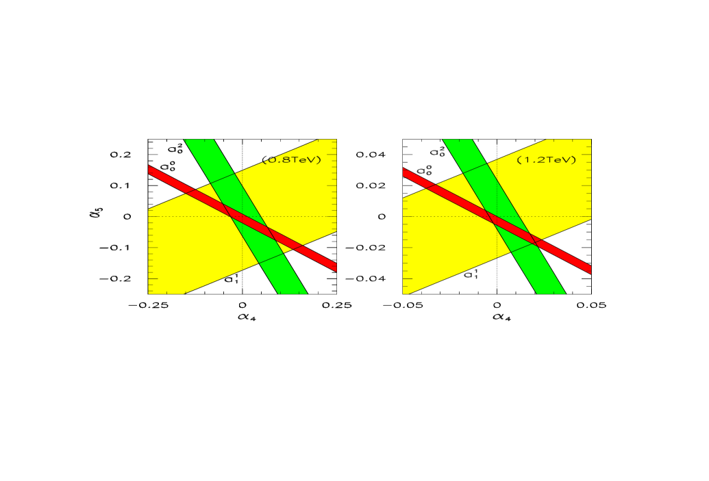
Figure 12: Region in $\alpha_{4,5}$ allowed by tree-level unitarity for $WW$ elastic scattering at a subprocess energy of $0.8\;{\rm TeV}$ (left) resp. $1.2\;{\rm TeV}$ (right).

Two-body elastic unitarity requires $|a_{\ell}^{I}-\frac{i}{2}|=1/2$. Once a partial-wave amplitude approaches the limit ${\rm Re}\,a_{\ell}^{I}=1/2$, rescattering effects set in which induce a phase shift that unitarizes the amplitudes. Such effects can no longer be described within the effective-theory approach in a model-independent way. The validity of the chiral expansion is therefore limited to $WW$-scattering energies $\sqrt{\hat{s}}$ and values of the parameters $\alpha_{i}$ such that

$$|a_{\ell}^{I}|\lesssim 1/2$$ (73)

In Fig.12 we display the allowed region in the $[\alpha_{4},\alpha_{5}]$ plane for $\sqrt{\hat{s}}=0.8\;{\rm TeV}$ and $1.2\;{\rm TeV}$, which cover the main energy range of the $WW$ scattering subprocess in the analysis. The strongest limits can be derived from unitarity in the $S$-wave for isospin $0$ and $2$ channels. The limit from the $I=\ell=1$ channel is significantly weaker. As demonstrated in Fig.12, the unitarity bounds are very sensitive to the energy scale: For $\sqrt{\hat{s}}=1.2\;{\rm TeV}$ they are more stringent by about a factor of $5$ than the bounds at $0.8\;{\rm TeV}$. However, they only marginally restrict the $\alpha_{i}$ parameters in the range we are interested in ($|\alpha_{i}|\lesssim 0.005$). Thus they do not affect the validity of the chiral expansion in the range considered in the present analysis.

Appendix B Radiative corrections

The leading radiative corrections of the tree-level amplitude (26) are generated by the one-loop corrections from pure Goldstone dynamics (Fig.13). They give rise to additional $SU(2)_{c}$-symmetric contributions of the form [38]

$$\Delta A(s,t,u)_{\rm 1\;loop}=\frac{1}{16\pi^{2}v^{4}}\left\{-\frac{(t-u)}{6}\left[t\ln\frac{-t}{\mu^{2}}-u\ln\frac{-u}{\mu^{2}}\right]-\frac{s^{2}}{2}\ln\frac{-s}{\mu^{2}}\right\}$$ (74)

The real part of these corrections is taken to vanish at the symmetric point $\mu^{2}=s=-2t=-2u$, which corresponds to the scattering angle $\theta=\pi/2$. Infinities are absorbed in the definition of the renormalized parameters $\alpha_{4,5}(\mu)$. A shift in the scale $\mu$ may be mapped into a finite renormalization of the parameters $\{\alpha_{4},\alpha_{5}\}$:

$$\alpha_{4}(\mu) = \alpha_{4}(\mu_{0})-\frac{1}{16\pi^{2}}\,\frac{1}{6}\ln\frac{\mu}{\mu_{0}}$$ (75)

$$\alpha_{5}(\mu) = \alpha_{5}(\mu_{0})-\frac{1}{16\pi^{2}}\,\frac{1}{12}\ln\frac{\mu}{\mu_{0}}$$ (76)

The leading-order term $A(s,t,u)_{\rm LO}=s/v^{2}$ is not renormalized. The same holds true for the next-to-leading order custodial $SU(2)_{c}$-breaking coefficients $\alpha_{6,7,10}$ because standard one-loop corrections generate only $SU(2)_{c}$-symmetric amplitudes.

Figure 13: Leading one-loop contributions to the $WW$ scattering amplitude, expressed in terms of Goldstone-boson scattering.

The leading contributions are built up by Goldstone loops since contributions of transverse $W,Z$ bosons are suppressed by the electroweak gauge couplings and by reduced enhancement factors in the energy [33].

Figure 14: Comparison of the leading one-loop corrections $|{\rm Re}\,(\Delta A)|$ to the longitudinal $W^{+}W^{-}\to W^{+}W^{-}$ scattering amplitude, with the effects due to nonvanishing values of $\alpha_{4}$ resp. $\alpha_{5}$.

Since the loop corrections (74) will affect the final results, it is necessary to estimate their impact. In Fig.14 a comparison is presented between the various contributions to the elastic scattering of longitudinal polarized $W$ bosons, $A(W^{+}W^{-}\to W^{+}W^{-})$, as a function of the scattering angle. The magnitude of the loop corrections, evaluated at the renormalization point $\mu=\sqrt{\hat{s}}$, is confronted with the effects of the next-to-leading order corrections ${\cal L}_{4}$ and ${\cal L}_{5}$ on the scattering amplitude. The loop corrections are apparently significantly smaller than the chiral contributions for coefficients $\alpha_{4}$ and $\alpha_{5}=0.001$. Since this is the size of the sensitivity we are aiming at, cf. Fig.9, we can conclude that the longitudinal loop corrections do not invalidate the previous tree-level results.

Appendix C Decomposition of helicity amplitudes

The partial wave decomposition formula for the helicity amplitudes of the process

$$W^{a}_{\lambda_{1}}W^{b}_{\lambda_{2}}\to W^{c}_{\lambda_{3}}W^{d}_{\lambda_{4}}$$ (77)

is defined as [24]

$$A(\lambda_{1}\lambda_{2},\lambda_{3}\lambda_{4})=\exp[i(\lambda-\lambda^{\prime})\varphi]\sum_{J}A_{J}(\lambda_{1}\lambda_{2},\lambda_{3}\lambda_{4})\,d^{J}_{\lambda\lambda^{\prime}}(\theta)$$ (78)

where $\lambda\equiv\lambda_{1}-\lambda_{2}$, $\lambda^{\prime}\equiv\lambda_{3}-\lambda_{4}$; and

$$d^{J}_{\lambda\lambda^{\prime}}(\theta) = \sum_{s=0}^{J}(-)^{s}\frac{\left[(J+\lambda)!(J-\lambda)!(J+\lambda^{\prime})!(J-\lambda^{\prime})!\right]^{1/2}}{s!(J-s-\lambda)!(J-s+\lambda^{\prime})!(\lambda-\lambda^{\prime}+s)!}$$ (79)

$$\times\left(\cos\frac{\theta}{2}\right)^{2(J-s)+\lambda^{\prime}-\lambda}\left(-\sin\frac{\theta}{2}\right)^{2s+\lambda-\lambda^{\prime}}$$

Each $2\to 2$ gauge-boson scattering process is described by a total of $3^{4}=81$ helicity amplitudes. However, by applying C,P,T transformations, they can be reduced to a basic set of 17, 20, and 13 independent amplitudes for the processes $W^{+}W^{-}\to W^{+}W^{-}$, $W^{+}W^{-}\to ZZ$, and $W^{-}W^{-}\to W^{-}W^{-}$, respectively, which we present in tabular form. In Tab.4–5 the contributions $A_{i}$ to the individual helicity amplitudes which are proportional to the NLO coefficients $\alpha_{i}$ are listed. In Tab.7–8 the $s$-, $t$-channel exchange, and contact terms are presented in LO for the main process $W^{+}W^{-}\to W^{+}W^{-}$. We use the notation

$$A_{J}=\left(\frac{E}{M_{W}}\right)^{e_{L}}\left[\sum_{V}g_{V}^{2}\left(\frac{p^{2}}{s-M_{V}^{2}}\hat{A}_{s}+\frac{E^{2}}{t-M_{V}^{2}}\hat{A}_{t}+\frac{E^{2}}{u-M_{V}^{2}}\hat{A}_{u}\right)+g^{2}\hat{A}_{c}+g^{4}\sum_{i=4,5}\alpha_{i}\hat{A}_{i}\right]$$ (80)

and

$$\beta\equiv p/E\qquad\beta_{W}\equiv p/E_{W}\qquad\beta_{Z}\equiv p/E_{Z}$$ (81)

where $p=|\vec{p}\,|$ is the length of 3-momentum of each incoming $W(Z)$ boson in the c.m. frame, and $E_{W}(E_{Z})$ is the corresponding c.m. energy. When the two incoming gauge bosons have equal masses, we remove the subscript of $E_{W}$ or $E_{Z}$. The vector boson masses and couplings are denoted by $M_{V},g_{V}$ ($V=W,Z,\gamma$ referring to the exchanged particle), where

$$g_{W}\equiv g=e/s_{w}\qquad g_{Z}=ec_{w}^{2}/s_{w}\qquad g_{\gamma}=e$$ (82)

with $s_{w}=\sin\theta_{w}$, $c_{w}=\cos\theta_{w}$.

$$\begin{array}[]{|l||c|c|c||c|c|c|}\hline\cr&\lx@intercol\hfil\alpha_{4}\hfil\lx@intercol\vrule\lx@intercol\vrule\lx@intercol&\lx@intercol\hfil\alpha_{5}\hfil\lx@intercol\vrule\lx@intercol\\ \hline\cr&J=0&1&2&0&1&2\\ \hline\cr\hline\cr\hat{A}^{J}_{i}(00,00)&{2(1+\beta^{2}+2\beta^{4})}&{2\beta^{2}}&{2}&{\frac{4}{3}(2+3\beta^{2}+3\beta^{4})}&{-4\beta^{2}}&{\frac{4}{3}}\\ \hline\cr\hat{A}^{J}_{i}(+0,00)&{-}&{-\beta^{2}}&{-\sqrt{3}}&{-}&{2\beta^{2}}&{-\frac{2}{\sqrt{3}}}\\ \hat{A}^{J}_{i}(++,00)&{-(2+\beta^{2})}&{-}&{1}&{-\frac{2}{3}(4+3\beta^{2})}&{-}&{\frac{2}{3}}\\ \hat{A}^{J}_{i}(+0,0+)&{-}&{-\frac{1}{2}+2\beta^{2}}&{3}&{-}&{2}&{1}\\ \hat{A}^{J}_{i}(+0,+0)&{-}&{-{1\over 2}-\beta^{2}}&{3\over 2}&{-}&{1-2\beta^{2}}&{1}\\ \hat{A}^{J}_{i}(+0,-0)&{-}&{-{1\over 2}+\beta^{2}}&{-{3\over 2}}&{-}&{1+2\beta^{2}}&{-1}\\ \hat{A}^{J}_{i}(+0,0-)&{-}&{-{1\over 2}-2\beta^{2}}&{-{3\over 2}}&{-}&{1}&{-1}\\ \hat{A}^{J}_{i}(+-,00)&{-}&{-}&{-\sqrt{6}}&{-}&{-}&{-{2\over 3}\sqrt{6}}\\ \hline\cr\hat{A}^{J}_{i}(++,+0)&{-}&{-{1\over 2}}&{\sqrt{3}\over 2}&{-}&{1}&{1\over\sqrt{3}}\\ \hat{A}^{J}_{i}(++,-0)&{-}&{1\over 2}&{\sqrt{3}\over 2}&{-}&{-1}&{1\over\sqrt{3}}\\ \hat{A}^{J}_{i}(+-,+0)&{-}&{-}&{3\over\sqrt{2}}&{-}&{-}&{\sqrt{2}}\\ \hat{A}^{J}_{i}(+-,0+)&{-}&{-}&{3\over\sqrt{2}}&{-}&{-}&{\sqrt{2}}\\ \hline\cr\hat{A}^{J}_{i}(++,++)&{2}&{-{1\over 2}}&{1\over 2}&{8\over 3}&{1}&{1\over 3}\\ \hat{A}^{J}_{i}(++,+-)&{-}&{-}&{-{\sqrt{6}\over{2}}}&{-}&{-}&{-{\sqrt{6}\over{3}}}\\ \hat{A}^{J}_{i}(++,--)&{2}&{1\over 2}&{1\over 2}&{8\over 3}&{-1}&{1\over 3}\\ \hat{A}^{J}_{i}(+-,-+)&{-}&{-}&{3}&{-}&{-}&{2}\\ \hat{A}^{J}_{i}(+-,+-)&{-}&{-}&{3}&{-}&{-}&{2}\\ \hline\cr\end{array}$$

Table 4: Decomposition of the NLO helicity amplitudes for $W^{+}W^{-}\rightarrow W^{+}W^{-}$.

$$\begin{array}[]{|c||c|c|c||c|c|c|}\hline\cr&\lx@intercol\hfil\alpha_{46}=\alpha_{4}+\alpha_{6}\hfil\lx@intercol\vrule\lx@intercol\vrule\lx@intercol&\lx@intercol\hfil\alpha_{57}=\alpha_{5}+\alpha_{7}\hfil\lx@intercol\vrule\lx@intercol\\ \hline\cr&{J=0}&{1}&{2}&{0}&{1}&{2}\\ \hline\cr\hline\cr\hat{A}^{J}_{i}(00,00)&{{2\over 3}+2\beta_{W}^{2}\beta_{Z}^{2}}&{-}&{{4\over 3}}&{2(1+\beta_{W}^{2}\beta_{Z}^{2}+\beta_{W}^{2}+\beta_{Z}^{2})}&{-}&{-}\\ \hline\cr\hat{A}^{J}_{i}(+0,00)&{-}&{-}&{-{2\over\sqrt{3}}}&{-}&{-}&{-}\\ \hat{A}^{J}_{i}(00,0+)&{-}&{-}&{-{2\over\sqrt{3}}c_{w}^{-1}}&{-}&{-}&{-}\\ \hat{A}^{J}_{i}(++,00)&{-{2\over 3}}&{-}&{{2\over 3}}&{-2(1+\beta_{Z}^{2})}&{-}&{-}\\ \hat{A}^{J}_{i}(00,++)&{{2\over 3}{c_{w}^{-2}}}&{-}&{{2\over 3}c_{w}^{-2}}&{-2(1+\beta_{Z}^{2})c_{w}^{-2}}&{-}&{-}\\ \hat{A}^{J}_{i}(00,+-)&{-}&{-}&{-\frac{4}{\sqrt{6}}c_{w}^{-2}}&{-}&{-}&{-}\\ \hat{A}^{J}_{i}(+-,00)&{-}&{-}&{-\frac{4}{\sqrt{6}}}&{-}&{-}&{-}\\ \hat{A}^{J}_{i}(+0,0-)&{-}&{-c_{w}^{-1}\beta_{W}\beta_{Z}}&{-c_{w}^{-1}}&{-}&{-}&{-}\\ \hat{A}^{J}_{i}(+0,0+)&{-}&{c_{w}^{-1}\beta_{W}\beta_{Z}}&{c_{w}^{-1}}&{-}&{-}&{-}\\ \hline\cr\hat{A}^{J}_{i}(++,+0)&{-}&{-}&{-\frac{1}{\sqrt{3}}c_{w}^{-1}}&{-}&{-}&{-}\\ \hat{A}^{J}_{i}(+0,++)&{-}&{-}&{-\frac{1}{\sqrt{3}}c_{w}^{-2}}&{-}&{-}&{-}\\ \hat{A}^{J}_{i}(++,0-)&{-}&{-}&{{1\over\sqrt{3}}c_{w}^{-1}}&{-}&{-}&{-}\\ \hat{A}^{J}_{i}(0-,++)&{-}&{-}&{{1\over\sqrt{3}}c_{w}^{-1}}&{-}&{-}&{-}\\ \hat{A}^{J}_{i}(0+,+-)&{-}&{-}&{\sqrt{2}c_{w}^{-2}}&{-}&{-}&{-}\\ \hat{A}^{J}_{i}(+-,0+)&{-}&{-}&{\sqrt{2}c_{w}^{-1}}&{-}&{-}&{-}\\ \hline\cr\hat{A}^{J}_{i}(++,++)&{{2\over 3}c_{w}^{-2}}&{-}&{\frac{1}{3}c_{w}^{-2}}&{2c_{w}^{-2}}&{-}&{-}\\ \hat{A}^{J}_{i}(++,--)&{{2\over 3}c_{w}^{-2}}&{-}&{\frac{1}{3}c_{w}^{-2}}&{2c_{w}^{-2}}&{-}&{-}\\ \hat{A}^{J}_{i}(++,+-)&{-}&{-}&{-{\sqrt{6}\over 3}c_{w}^{-2}}&{-}&{-}&{-}\\ \hat{A}^{J}_{i}(+-,++)&{-}&{-}&{-{\sqrt{6}\over 3}c_{w}^{-2}}&{-}&{-}&{-}\\ \hat{A}^{J}_{i}(+-,-+)&{-}&{-}&{2c_{w}^{-2}}&{-}&{-}&{-}\\ \hline\cr\end{array}$$

Table 5: Decomposition of the NLO helicity amplitudes for $W^{+}W^{-}\to ZZ$.

$$\begin{array}[]{|c||c|c|c||c|c|c|}\hline\cr&\lx@intercol\hfil\alpha_{4}\hfil\lx@intercol\vrule\lx@intercol\vrule\lx@intercol&\lx@intercol\hfil\alpha_{5}\hfil\lx@intercol\vrule\lx@intercol\\ \hline\cr&{J=0}&{1}&{2}&{0}&{1}&{2}\\ \hline\cr\hline\cr\hat{A}^{J}_{i}(00,00)&{4(\frac{2}{3}+\beta^{2}+\beta^{4})}&{-}&{{4\over 3}}&{4(\frac{1}{3}+\beta^{4})}&{-}&{\frac{8}{3}}\\ \hline\cr\hat{A}^{J}_{i}(+0,00)&{-}&{-}&{-\frac{2}{\sqrt{3}}}&{-}&{-}&{\frac{4}{\sqrt{3}}}\\ \hline\cr\hat{A}^{J}_{i}(++,00)&{-\frac{2}{3}(4+3\beta^{2})}&{-}&{-\frac{2}{3}}&{-\frac{4}{3}}&{-}&{\frac{4}{3}}\\ \hat{A}^{J}_{i}(+0,0+)&{-}&{\beta^{2}}&{1}&{-}&{2\beta^{2}}&{2}\\ \hat{A}^{J}_{i}(00,+-)&{-}&{-}&{-\frac{4}{\sqrt{6}}}&{-}&{-}&{-\frac{8}{\sqrt{6}}}\\ \hat{A}^{J}_{i}(+0,0-)&{-}&{-\beta^{2}}&{-1}&{-}&{-2\beta^{2}}&{-2}\\ \hline\cr\hat{A}^{J}_{i}(++,+0)&{-}&{-}&{-\frac{1}{\sqrt{3}}}&{-}&{-}&{-2\over\sqrt{3}}\\ \hat{A}^{J}_{i}(++,0-)&{-}&{-}&{1\over\sqrt{3}}&{-}&{-}&{2\over\sqrt{3}}\\ \hat{A}^{J}_{i}(0+,+-)&{-}&{-}&{\sqrt{2}}&{-}&{-}&{2\sqrt{2}}\\ \hline\cr\hat{A}^{J}_{i}(++,++)&{\frac{8}{3}}&{-}&{1\over 3}&{3\over 2}&{-}&{2\over 3}\\ \hat{A}^{J}_{i}(++,+-)&{-}&{-}&{-{\sqrt{6}\over{3}}}&{-}&{-}&{-{2\sqrt{6}\over{3}}}\\ \hat{A}^{J}_{i}(++,--)&{8\over 3}&{-}&{1\over 3}&{4\over 3}&{-}&{2\over 3}\\ \hat{A}^{J}_{i}(+-,-+)&{-}&{-}&{2}&{-}&{-}&{4}\\ \hline\cr\end{array}$$

Table 6: Decomposition of the NLO helicity amplitudes for $W^{\pm}W^{\pm}\to W^{\pm}W^{\pm}$.

$$\begin{array}[]{|c||c|c|c||c|c|c|}\hline\cr&\vrule\lx@intercol\hfil\mbox{Contact graph}\hfil\lx@intercol\vrule\lx@intercol\vrule\lx@intercol&\vrule\lx@intercol\hfil\mbox{$s$-channel $Z/\gamma$--exchange}\hfil\lx@intercol\vrule\lx@intercol\\ \hline\cr&{J=0}&{1}&{2}&{0}&{1}&{2}\\ \hline\cr\hline\cr\hat{A}^{J}_{i}(00,00)&{-\frac{2}{3}(1+\beta^{2})}&{6\beta^{2}}&{\frac{2}{3}}&{-}&{-4(3-\beta^{2})^{2}}&{-}\\ \hline\cr\hat{A}^{J}_{i}(+0,00)&{-}&{-3\beta^{2}}&{-\frac{1}{\sqrt{3}}}&{-}&{8(3-\beta^{2})}&{-}\\ \hat{A}^{J}_{i}(++,00)&{\frac{2}{3}+\beta^{2}}&{-}&{1\over 3}&{-}&{4(\beta^{2}-3)}&{-}\\ \hat{A}^{J}_{i}(+0,0+)&{-}&{-\frac{3}{2}+2\beta^{2}}&{1\over 2}&{-}&{-16}&{-}\\ \hat{A}^{J}_{i}(+0,+0)&{-}&{-{3\over 2}+\beta^{2}}&{1\over 2}&{-}&{-16}&{-}\\ \hat{A}^{J}_{i}(+0,-0)&{-}&{-{3\over 2}-\beta^{2}}&{-{1\over 2}}&{-}&{16}&{-}\\ \hat{A}^{J}_{i}(+0,0-)&{-}&{-{3\over 2}-2\beta^{2}}&{-{1\over 2}}&{-}&{16}&{-}\\ \hat{A}^{J}_{i}(+-,00)&{-}&{-}&{\frac{\sqrt{6}}{3}}&{-}&{-}&{-}\\ \hline\cr\hat{A}^{J}_{i}(++,+0)&{-}&{{3\over 2}}&{-\frac{\sqrt{3}}{6}}&{-}&{8}&{-}\\ \hat{A}^{J}_{i}(++,-0)&{-}&{3\over 2}&{\sqrt{3}\over 6}&{-}&{-8}&{-}\\ \hat{A}^{J}_{i}(+-,+0)&{-}&{-}&{1\over\sqrt{2}}&{-}&{-}&{-}\\ \hat{A}^{J}_{i}(+-,0+)&{-}&{-}&{1\over\sqrt{2}}&{-}&{-}&{-}\\ \hline\cr\hat{A}^{J}_{i}(++,++)&{-\frac{2}{3}}&{-{3\over 2}}&{1\over 6}&{-}&{-4}&{-}\\ \hline\cr\hat{A}^{J}_{i}(++,+-)&{-}&{-}&{-\frac{1}{\sqrt{6}}}&{-}&{-}&{-}\\ \hat{A}^{J}_{i}(++,--)&{-\frac{2}{3}}&{3\over 2}&{1\over 6}&{-}&{-4}&{-}\\ \hat{A}^{J}_{i}(+-,-+)&{-}&{-}&{1}&{-}&{-}&{-}\\ \hat{A}^{J}_{i}(+-,+-)&{-}&{-}&{1}&{-}&{-}&{-}\\ \hline\cr\end{array}$$

Table 7: Decomposition of the NLO helicity amplitudes for $W^{+}W^{-}\to W^{+}W^{-}$.

$$\begin{array}[]{|c||c|c|c|c|}\hline\cr&\vrule\lx@intercol\hfil\mbox{$t$-channel $Z/\gamma$-exchange}\hfil\lx@intercol\vrule\lx@intercol\\ \hline\cr&{J=0}&{1}&{2}&{3}\\ \hline\cr\hline\cr\hat{A}^{J}_{t}(00,00)&{-10(2+\beta^{2}+4\beta^{4}+\beta^{6})}&{6\beta^{2}(-23+50\beta^{2}-5\beta^{4})}&{20(-2+11\beta^{2}-10\beta^{4})}&{-12\beta^{2}}\\ \hline\cr\hat{A}^{J}_{t}(+0,00)&{-}&{18\beta^{2}(7-5\beta^{2})}&{10\sqrt{3}(2-9\beta^{2}+5\beta^{4})}&{4\sqrt{6}\beta^{2}}\\ \hat{A}^{J}_{t}(++,00)&{20(2-3\beta^{2}+2\beta^{4})}&{-114\beta^{2}}&{20(-2+9\beta^{2}-2\beta^{4})}&{-6\beta^{2}}\\ \hat{A}^{J}_{t}(+0,0+)&{-}&{-6(5+17\beta^{2}+5\beta^{4})}&{10(-3+13\beta^{2}-3\beta^{4})}&{-8\beta^{2}}\\ \hat{A}^{J}_{t}(+0,+0)&{-}&{3(-10-39\beta^{2}+25\beta^{4})}&{5(-6+25\beta^{2}-3\beta^{4})}&{-8\beta^{2}}\\ \hat{A}^{J}_{t}(+0,-0)&{-}&{3(-10+39\beta^{2}-5\beta^{4})}&{5(6-17\beta^{2}+3\beta^{4})}&{8\beta^{2}}\\ \hat{A}^{J}_{t}(+0,0-)&{-}&{6(-5+12\beta^{2}-5\beta^{4})}&{10(3-8\beta^{2}+3\beta^{4})}&{8\beta^{2}}\\ \hat{A}^{J}_{t}(+-,00)&{-}&{-}&{10\sqrt{6}(2-5\beta^{2}+2\beta^{4})}&{2\sqrt{30}\beta^{2}}\\ \hline\cr\hat{A}^{J}_{t}(++,+0)&{-}&{6(5+13\beta^{2})}&{10\sqrt{3}(1-5\beta^{2})}&{2\sqrt{6}\beta^{2}}\\ \hat{A}^{J}_{t}(++,-0)&{-}&{6(5-8\beta^{2})}&{10\sqrt{3}(-1+2\beta^{2})}&{-2\sqrt{6}\beta^{2}}\\ \hat{A}^{J}_{t}(+-,+0)&{-}&{-}&{10\sqrt{2}(-3+4\beta^{2})}&{-4\sqrt{5}\beta^{2}}\\ \hat{A}^{J}_{t}(+-,0+)&{-}&{-}&{10\sqrt{2}(-3+5\beta^{2})}&{-4\sqrt{5}\beta^{2}}\\ \hline\cr\hat{A}^{J}_{t}(++,++)&{-5(4+19\beta^{2})}&{-3(10+9\beta^{2})}&{5(-2+13\beta^{2})}&{-3\beta^{2}}\\ \hat{A}^{J}_{t}(++,+-)&{-}&{-}&{5\sqrt{6}(2-3\beta^{2})}&{\sqrt{30}\beta^{2}}\\ \hat{A}^{J}_{t}(++,--)&{-5(4+\beta^{2})}&{3(10+\beta^{2})}&{5(-2+\beta^{2})}&{-3\beta}\\ \hat{A}^{J}_{t}(+-,-+)&{-}&{-}&{-10(6+\beta^{2})}&{-10\beta^{2}}\\ \hat{A}^{J}_{t}(+-,+-)&{-}&{-}&{-10(6+5\beta^{2})}&{-10\beta^{2}}\\ \hline\cr\end{array}$$

Table 8: Decomposition of the leading order helicity amplitudes for $W^{+}W^{-}\to W^{+}W^{-}$.

References

[1]
B. Lee, C. Quigg and H. Thacker,
Phys. Rev. Lett. 38, 883 (1977);
Phys. Rev. D16, 1519 (1977);
D. Dicus and V. Mathur, Phys. Rev. D7, 3111 (1973).
[2]
S. Glashow,
Nucl. Phys. 22, 579 (1961);
A. Salam, in: Elementary Particle Theory,
ed. N. Svartholm (1968);
S. Weinberg,
Phys. Rev. Lett. 19, 1264 (1967).
[3]
P.W. Higgs,
Phys. Lett. 12, 132 (1964);
Phys. Rev. Lett. 13, 508 (1964);
Phys. Rev. 145, 1156 (1966);
F. Englert and R. Brout,
Phys. Rev. Lett. 13, 321 (1964);
G.S. Guralnik, C.R. Hagen, and T.W.B. Kibble,
Phys. Rev. Lett. 13, 585 (1964);
T.W.B. Kibble,
Phys. Rev. 155, 1554 (1967).
[4]
C.H. Llewellyn Smith,
Phys. Lett. B46, 233 (1973);
J.M. Cornwall, D.N. Levin, and G. Tiktopoulos,
Phys. Rev. D10, 1145 (1974),
E: D11, (1975) 972.
[5]
A. Blondel, in:
Proceedings of Int. Conference on High Energy Physics,
Warsaw 1996.
[6]
U. Baur and M. Demarteau, in:
Proceedings of the DPF/DPB Summer Study,
Snowmass 1996.
[7]
M.E. Peskin and T. Takeuchi,
Phys. Rev. Lett. 65, 964 (1990);
Phys. Rev. D46, 381 (1992).
[8]
K.J.F. Gaemers, G.J. Gounaris,
Z. Phys. C1, 259 (1979);
K. Hagiwara, K. Hikasa, R.D. Peccei, and D. Zeppenfeld,
Nucl. Phys. B282, 253 (1987);
G.J. Gounaris, J.L. Kneur, D. Zeppenfeld et al.,
Triple Gauge Boson Couplings, in CERN 96-01.
[9]
R. Casalbuoni, S. De Curtis, and D. Dominici,
Phys. Lett. B403, 86 (1997).
[10]
G. Bélanger and F. Boudjema,
Phys. Lett. B288, 201 (1992);
S. Dawson, A. Likhoded, G. Valencia, and O. Yushchenko,
in: Proceedings of the DPF/DPB Summer Study,
Snowmass 1996, hep-ph/9610299.
[11]
S. Weinberg,
Phys. Rev. D13, 974 (1976);
ibid.D19, 1277 (1979);
L. Susskind,
Phys. Rev. D20, 2619 (1979).
[12]
M. Veltman,
Act. Phys. Pol. B8, 475 (1977);
Nucl. Phys. B123, 89 (1977);
P. Sikivie, L. Susskind, M. Voloshin, and V. Zakharov,
Nucl. Phys. B173, 189 (1980).
[13]
C.E. Vayonakis,
Lett. Nuovo Cim. 17, 383 (1976);
M.S. Chanowitz and M.K. Gaillard,
Nucl. Phys. B261, 379 (1985);
G.J. Gounaris, R. Kögerler, and H. Neufeld,
Phys. Rev. D34, 3257(1986);
Y.-P. Yao and C.-P. Yuan,
ibid.D38, 2237 (1988);
J. Bagger and C. Schmidt,
ibid.D34, 264 (1990).
[14]
H.-J. He, Y.-P. Kuang, and X.-Y. Li,
Phys. Rev. Lett. 69, 2619 (1992);
Phys. Lett. B329, 278 (1994);
Phys. Rev. D49, 4842 (1994);
H.-J. He, Y.-P. Kuang, and C.-P. Yuan,
ibid.D51, 6463 (1995);
H.-J. He and W.B. Kilgore,
ibid.D55, 1515 (1997).
[15]
H. Veltman,
Phys. Rev. D41, 2294 (1990);
W.B. Kilgore,
Phys. Lett. B294, 257 (1992);
A. Dobado and J.R. Pelaez,
ibid.B329, 469 (1994),
E: B335, 554 (1994);
J. Horejsi,
Preprint PRA-HEP-95/9, hep-ph/9603321;
C. Grosse-Knetter and I. Kuss,
Z. Phys. C95, 66 (1995);
J.F. Donoghue and J. Tandean,
Phys. Lett. B361, 69 (1995);
T. Torma,
Phys. Rev. D54, 2168 (1996);
A. Denner and S. Dittmaier,
ibid.D54, 4499 (1996);
and references therein.
[16]
E. Accomando et al.
(ECFA/DESY LC Physics Working Group), DESY-97-100,
hep-ph/9705442.
[17]
V. Barger, K. Cheung, T. Han, and R.J.N. Phillips,
Phys. Rev. D52, 3815 (1995).
[18]
F. Cuypers and K. Kolodziej,
Phys. Lett. B344, 365 (1995);
F. Cuypers,
Int. J. Mod. Phys. A11, 1525 (1996).
[19]
T. Han,
Int. J. Mod. Phys. A11, 1541 (1996).
[20]
W. Kilian, in:
Proceedings of the DPF/DPB Summer Study,
Snowmass 1996, hep-ph/9609334;
H.-J. He, DESY-97-037, in:
Proceedings of the Workshop:
The Higgs Puzzle — What Can We Learn
From LEP2, LHC, NLC, and FMC?,
Ringberg 1996,
World Scientific.
[21]
J. Gasser and H. Leutwyler,
Ann. Phys. (N.Y.) 158, 142 (1984);
Nucl. Phys. B250, 465 (1985).
[22]
T. Appelquist and C. Bernard,
Phys. Rev. D22, 200(1980);
A. Longhitano,
Phys. Rev. D22, 1166 (1980);
Nucl. Phys. B188, 118 (1981);
T. Appelquist and G.-H. Wu,
Phys. Rev. D48, 3235 (1993).
[23]
S. Weinberg,
Physica 96A, 327 (1979);
H. Georgi,
Weak interactions and modern particle theory,
Benjamin/Cummings 1984;
A. Manohar and H. Georgi,
Nucl. Phys. B234, 189 (1984).
[24]
M. Jacob and G.C. Wick,
Ann. Phys. 7, 404 (1959).
[25]
M.S. Chanowitz and M.K. Gaillard,
Phys. Lett. B142, 85 (1984);
G.L. Kane, W.W. Repko, and W.R. Rolnick,
Phys. Lett. B148, 367 (1984);
S. Dawson,
Nucl. Phys. B249, 42 (1985);
J. Lindfors, Z. Phys. C28, 427 (1985);
J.F. Gunion, J. Kalinowski, and A. Tofighi-Niaki,
Phys. Rev. Lett. 57, 2351 (1986).
[26]
E. Fermi, Z. Phys. 29, 315 (1924);
E.J. Williams,
Proc. Roy. Soc. A139, 163 (1933);
Phys. Rev. 45, 729 (1934);
C.F. von Weizsäcker,
Z. Phys. 88, 612 (1934).
[27]
M.S. Chen and P.M. Zerwas,
Phys. Rev. D11, 58 (1975).
[28]
I. Kuss and H. Spiesberger,
Phys. Rev. D53, 6078 (1996);
I. Kuss, Phys. Rev. D55, 7165 (1997).
[30]
J.F. Gunion, J. Kalinowski, and A. Tofighi-Niaki,
Phys. Rev. Lett. 57, 2351 (1986);
[31]
I. Kuss, Phys. Rev. D55, 7165 (1997);
I. Kuss and E. Nuss, hep-ph/9706406.
[32]
E.E. Boos, M.N. Dubinin, V.A. Ilyin,
A.E. Pukhov, and V.I. Savrin,
Report SNUTP–94–116, hep-ph/9503280 (unpublished);
P.A.Baikov et al.,
in: Proceedings of the Workshop QFTHEP-96,
eds. B. Levtchenko and V. Savrin
(Moscow 1996), hep-ph/9701412.
[33]
H.-J. He, Y.-P. Kuang, and C.-P. Yuan,
Phys. Rev. D55, 3038 (1997);
Lectures in the Proceedings of the CCAST (World Laboratory) Workshop
on Physics at TeV Energy Scale72, 119,
Beijing 1996,
DESY-97-056, hep-ph/9704276;
and references therein.
[34]
O.J.P. Eboli, et al,
Phys. Lett. B339, 119 (1995); B375, 233 (1996);
S. Dawson and G. Valencia, Nucl. Phys. B439, 3 (1995).
[35]
A. Dobado, M.J. Herrero, J.R. Pelaez, E. Ruiz Morales,
and M.T. Urdiales,
Phys. Lett. B352, 400 (1995);
A. Dobado and M.T. Urdiales,
Z. Phys. C71, 659 (1996).
[36]
J. Bagger, V. Barger, K. Cheung,
J. Gunion, T. Han, G.A. Ladinsky, R. Rosenfeld, and C.-P. Yuan,
Phys. Rev. D49, 1246 (1994);
ibid.D52, 3878 (1995).
[37]
V. Barger, M.S. Berger, J.F. Gunion, and T. Han,
Phys. Rep. 286, 1 (1997);
Phys. Rev. D55, 142 (1997);
J.F. Gunion,
Preprint UCD 97-17, hep-ph/9707379.
[38]
O. Cheyette and M.K. Gaillard,
Phys. Lett. B197, 205 (1987).