[

Primordial magnetic fields, anomalous isocurvature fluctuations
and Big Bang nucleosynthesis

Abstract

We show that the presence of primordial stochastic (hypercharge) magnetic fields before the electroweak (EW) phase transition induces isocurvature fluctuations (baryon number inhomogeneities). Depending on the details of the magnetic field spectrum and on the particle physics parameters (such as the strength of the EW phase transition and electron Yukawa couplings) these fluctuations may survive until the Big Bang nucleosynthesis (BBN). Their lenghtscale may exceed the neutron diffusion length at that time, while their magnitude can be so large that sizable antimatter domains are present. This provides the possibility of a new type of initial conditions for non-homogeneous BBN or, from a more conservative point of view, stringent bounds on primordial magnetic fields.

CERN-TH/97-138, hep-ph/9708303

]

Large scale magnetic fields in diffuse astrophysical plasmas represent a well established observational fact since few decades. It has been realized through the years that magnetic fields coherent over diverse length scales at different epochs may have a variety of quite interesting phenomenological consequences. Magnetic fields coherent today over scales of the order of 30 Kpc are measured [1] and have an important role in the dynamics of the galaxy, for example, in confining cosmic rays [2]. Magnetic fields at the nucleosynthesis epoch, even if not directly observable, could change the reaction and the expansion rate at that time. The success of the homogeneous and isotropic BBN provides then interesting bounds on their existence [3].

There are neither compelling theoretical arguments nor motivated phenomenological constraints which could exclude the existence of magnetic fields prior to the nucleosynthesis epoch. Moreover, to explain the origin of the galactic magnetic fields some authors often invoke the dynamo mechanism which might amplify the primordial “seed” magnetic field. It is a challenge to produce large scale seeds, and different ideas were aimed at this purpose. The energy scales involved vary from $\sim 100$ MeV for the QCD phase transition [4] to $\sim 100$ GeV in the case of the EW physics [5, 6] and even closer to the Planck energy scale for inflation or string cosmology [7, 8].

The purpose of this Letter is the study of the implications of the primordial magnetic fields which existed even before the EW scale (i. e. for temperatures $\raise 1.29167pt\hbox{$>$\kern-7.5pt\raise-4.73611pt\hbox{$\sim$}}100$ GeV). The origin of these seeds is not essential for us and consequently we simply assume that they were generated by some mechanism before the EW phase transition. Our main point is that these fields produce baryon and lepton number inhomogeneities (isocurvature fluctuations), which could have an impact on the standard BBN.

Let us start from some qualitative considerations. A unique property of “unbroken” U(1) gauge interaction is the absence of mass of its corresponding vector particle. Static “magnetic” fields are never screened (in the absence of monopoles) and thus homogeneous fields can survive in the plasma for infinite time. Under normal conditions (i.e. small temperatures and small densities of the different fermionic charges) the SU(2)$\times$U(1)_Y symmetry is “broken” down to U(1)_EM, the massless field corresponding to U(1)_EM is the ordinary photon and the only long-lived field in the plasma is the ordinary magnetic one. At sufficiently high temperatures $T>T_{c}$, the SU(2)$\times$U(1)_Y symmetry is “restored”, and non-screened vector modes $Y_{\mu}$ correspond to the U(1)_Y hypercharge group. Hence, if primordial fields existed at $T>T_{c}$, they did correspond to hypercharge rather that U(1)_EM. There are essential differences between the interactions of magnetic fields and the ones of hyper-magnetic fields with matter. The ordinary electro-magnetic field has a vector-like coupling to the fermions, while the coupling of the hypercharge fields is chiral. Thus, if hyper-electric ($\vec{{\cal E}}_{Y}$) and hyper-magnetic ($\vec{{\cal H}}_{Y}$) fields are present simultaneously, they cause a variation of the fermionic number according to the anomaly equation, $\partial_{\mu}j_{\mu}\sim\frac{g^{\prime 2}}{4\pi^{2}}\vec{{\cal H}}_{Y}\cdot\vec{{\cal E}}_{Y}$ (here $g^{\prime}$ the hypercharge gauge coupling constant). Now, the presence of non-homogeneous hyper-magnetic fields in the EW plasma with (hyper) conductivity $\sigma_{c}$ always implies the existence of a related electric field, $\vec{{\cal E}}_{Y}\sim\frac{1}{\sigma_{c}}\vec{\nabla}\times\vec{{\cal H}}_{Y}$. Since for a general stochastic magnetic background $\langle(\vec{{\cal H}}_{Y}\cdot\vec{\nabla}\times\vec{{\cal H}}_{Y})^{2}\rangle\neq 0$, the non-uniform hyper-magnetic field must produce baryon and lepton density perturbations because of the anomaly equation. In what follows we compute the amplitude of isocurvature fluctuations induced by this mechanism and discuss their physical relevance.

The starting point of our discussion will be the generalization of the magneto-hydrodynamics (MHD) equations ( valid for ordinary electro-magnetic plasmas) to the case of hyper-magnetic fields with anomalous coupling to the fermionic degrees of freedom (see also [6]). These equations have to be used for $T>T_{c}$. We are interested in a slow dynamics and we then assume that most of the particle reactions are in thermal equilibrium in the expanding Universe (the list of those include all perturbative strong and weak processes, strong and EW sphalerons, Yukawa interactions of $\mu$, $\tau$ and $s,~{}c,~{}b,~{}t$ quarks). The particle physics processes crucial for our purposes are those related to the U(1)_Y anomaly and to the slowest perturbative reactions with right electron chirality flip (e.g. $e_{R}+Higgs\rightarrow e_{L}+W$). Thus, our variables are the space-dependent hyper-magnetic and electric fields $\vec{{\cal H}}_{Y},~{}\vec{{\cal E}}_{Y}$ and right electron chemical potential $\mu_{R}(\vec{x})$. The generalized Maxwell equations in a Friedmann-Robertson-Walker metric with scale factor $a(\tau)$ are

$$\frac{\partial{{\vec{H}}_{Y}}}{\partial\tau}=-\vec{\nabla}\times{\vec{E}}_{Y},~{}~{}\frac{\partial{\vec{E}}_{Y}}{\partial\tau}+{\vec{J}}_{Y}=4\mu a{\vec{H}}_{Y}+{\vec{\nabla}}\times{\vec{H}}_{Y}$$ (1)

$${\vec{\nabla}}\cdot{\vec{H}}_{Y}=0,~{}~{}{\vec{\nabla}}\cdot{\vec{E}}_{Y}=0,~{}~{}{\vec{J}}_{Y}=\sigma{\vec{E}}_{Y},~{}a(\tau)d\tau=dt$$ (2)

($\vec{E}_{Y}=a^{2}\vec{{\cal E}}_{Y}$; $\vec{H}_{Y}=a^{2}\vec{{\cal H}}_{Y}$; $\vec{J_{Y}}=a^{3}\vec{j_{Y}}$; $\sigma=\sigma_{c}a$). A new term, proportional the right electron chemical potential, comes from the anomaly contribution to the effective Lagrangian of hypercharge gauge fields [9],

$$\delta{{\cal L}_{Y,e_{R}}} = \mu\epsilon_{ijk}Y^{ij}Y^{k}~{},$$ (3)

$$\mu = \frac{g^{\prime 2}}{4\pi^{2}}\mu_{R},~{}~{}Y_{\alpha\beta}=\partial_{[\alpha}Y_{\beta]}~{}.$$ (4)

Since the EW plasma conductivity is large, $\sigma_{c}\sim\sigma_{0}T$ with $\sigma_{0}\simeq 70~{}-~{}100$ [10], the time derivatives of the electric fields in Eq. (2) can be neglected (in the MHD context this is known as “resistive” approximation [11]). This observations allows to express the induced electric field in terms of the magnetic one,

$${\vec{{\cal E}}}_{Y}=\frac{{\vec{j}}_{Y}}{\sigma_{c}}\simeq\frac{1}{\sigma_{c}}\left(4~{}\mu~{}{\vec{{\cal H}}}_{Y}+{\vec{\nabla}}\times{\vec{{\cal H}}}_{Y}\right)~{}~{}~{},$$ (5)

and derive an equation for $\vec{{\cal H}}_{Y}$ only. It is interesting to note that the presence of the fermionic chemical potential induces an electric field parallel to the magnetic one.

The set of Eq. (2) has to be supplemented by the kinetic equation for the right electron chemical potential, which accounts for anomalous and perturbative non-conservation of the right electron number:

$$\frac{\partial}{\partial t}\left(\frac{\mu_{R}}{T}\right) = -\frac{g^{\prime 2}}{4\pi^{2}\sigma_{c}T^{3}}\frac{783}{88}{\vec{{\cal H}}}_{Y}\cdot\vec{\nabla}\times{\vec{{\cal H}}}_{Y}$$ (6)

$$- (\Gamma+\Gamma_{{\cal H}})\frac{\mu_{R}}{T},$$ (7)

where $\Gamma$ is the chirality changing rate,

$$\Gamma_{{\cal H}}=\frac{783}{22}\frac{\alpha^{\prime 2}}{\sigma_{c}\pi^{2}}\frac{|{\vec{{\cal H}}}_{Y}|^{2}}{T^{2}},~{}~{}~{}\alpha^{\prime}=\frac{g^{\prime 2}}{4\pi}~{}~{},$$ (8)

(the numbers $783/88$ and $783/22$ come from the relationship between $e_{R}$ number density and chemical potential [6]). An interesting consequence of Eqs. (7,8) is that in the presence of non-zero uniform magnetic field the right electron number is non-conserved (if $\Gamma=0$), even for an abelian anomaly (cf. Ref. [12]).

Now we are ready to compute baryon number fluctuations produced in our scenario. We notice that at the temperature of the EW phase transition $\sim 100$ GeV, $\Gamma t\gg 1$. Then, since reactions with right electron chirality flip are in the thermal equilibrium, the adiabatic approximation can be used, and from Eq. (7) we have

$$\frac{\mu_{R}}{T}\simeq-\frac{\alpha^{\prime}}{\pi\sigma_{c}T^{3}}\frac{783}{88}\frac{{\vec{{\cal H}}}_{Y}\cdot\vec{\nabla}\times{\vec{{\cal H}}}_{Y}}{\Gamma+\Gamma_{{\cal H}}}.$$ (9)

Clearly, a non-uniform distribution of the right electron chemical potential induces baryon and lepton number perturbations of the same order of magnitude. We are not going to write the explicit formulae since there is an important “storage” effect which amplifies the estimates of Eq. (9) by many orders of magnitude. Equations (5,7,9) imply that

$$\vec{{\cal H}}_{Y}\cdot\vec{{\cal E}}_{Y}\simeq\frac{\Gamma}{\Gamma+\Gamma_{{\cal H}}}\frac{1}{\sigma_{c}}{\vec{{\cal H}}}_{Y}\cdot\vec{\nabla}\times{\vec{{\cal H}}}_{Y}\neq 0~{}~{}.$$ (10)

Now, the change of Abelian Chern-Simons number is given by the time integral of (10). At the EW phase transition the hyper-magnetic fields are converted into ordinary magnetic fields. The latter do not have coupling to the anomaly. Thus the CS number has to be transformed into fermions according to Eq. (7). Inserting the coefficients, we arrive, from Eq. (10) at our main result:

$$\delta\left(\frac{n_{B}}{s}\right)(\vec{x},t_{c})=\frac{\alpha^{\prime}}{2\pi\sigma_{c}}\frac{n_{f}}{s}\frac{{\vec{{\cal H}}}_{Y}\cdot\vec{\nabla}\times{\vec{{\cal H}}}_{Y}}{\Gamma+\Gamma_{{\cal H}}}\frac{\Gamma M_{0}}{T_{c}^{2}}$$ (11)

($n_{B}$ and $s$ are the baryon and entropy densities, $s=\frac{2}{45}\pi^{2}N_{eff}T^{3}$, $N_{eff}$ is the effective number of massless degrees of freedom [$106.75$ for minimal standard model], $M_{0}=M_{pl}/1.66\sqrt{N_{eff}}\simeq 7.1\times 10^{17}$ GeV). Notice that in Eq. (11) there is an enhancement by a factor $\sim\Gamma M_{0}/T_{c}^{2}$ arising from the time integration of the anomaly term.

Some comments are now in order.

(i) For the correctness of Eq. (11) the EW phase transition should be strongly first order. Moreover, a necessary condition for EW baryogenesis [13] must be satisfied. In the opposite case all baryon number fluctuations will be erased by SU(2) sphalerons as it happens in the minimal standard model (MSM) [14], while this is not necessarily the case for the supersymmetric and other extensions of the standard model [15].

(ii) Besides the primordial hyper-magnetic field, an essential quantity which fixes the amplitude of the isocurvature fluctuations is the rate of perturbative right electron chirality flip, $\Gamma$. For $\Gamma_{H}\raise 1.29167pt\hbox{$>$\kern-7.5pt\raise-4.73611pt\hbox{$\sim$}}\Gamma$ the amplitude of baryon number fluctuations does not depend on the magnitude of the magnetic field fluctuations and it is determined just by their spectral slope. For $\Gamma_{H}\raise 1.29167pt\hbox{$<$\kern-7.5pt\raise-4.73611pt\hbox{$\sim$}}\Gamma$ the rate of right electron chirality flip cancels out and the isocurvature fluctuations are fixed both by the magnitude and by the spectral slope of the primordial magnetic fields. In the MSM the rate $\Gamma$ depends crucially upon the electron Yukawa coupling and is known to be $\Gamma=T\frac{T_{R}}{M_{0}}$, where $T_{R}\simeq 80$ TeV is the freezing temperature [16] of the right electrons. This number appears to be too small to allow any interesting fluctuations. However, in the extensions of the standard model the rate $\Gamma$ is naturally larger than in MSM. For example, in the MSSM the right-electrons Yukawa coupling is larger by a factor $1/\cos{\beta}$, which may increase the value of $T_{R}$ by 3 orders of magnitude for experimentally allowed $\tan(\beta)\sim 50$. Cosmologically interesting fluctuations arise at $T_{R}>T^{*}\simeq 10^{5}$ TeV [17].

We will assume now that $\Gamma\raise 1.29167pt\hbox{$>$\kern-7.5pt\raise-4.73611pt\hbox{$\sim$}}\Gamma_{H}$, but similar conclusions hold true for the case $\Gamma\raise 1.29167pt\hbox{$<$\kern-7.5pt\raise-4.73611pt\hbox{$\sim$}}\Gamma_{H}$ and $T_{R}>T^{*}$ (for details see [17]). In order to compute the amplitude and the spectrum of the baryon number fluctuations we will also suppose that the Fourier modes of the magnetic fields are stochastically distributed, leading to a rotationally and parity invariant two-point function

$$G_{ij}(r)=\langle H_{i}(\vec{x})H_{j}(\vec{x}+\vec{r})\rangle~{}~{},$$ (12)

where $\langle...\rangle$ denotes an ensemble average. In this case $\langle\delta\left(\frac{n_{B}}{s}\right)(\vec{x},t)\rangle=0$ [18], but

$$\Delta(r,t_{c})=\sqrt{\langle\delta\left(\frac{n_{B}}{s}\right)(\vec{x},t_{c})\delta\left(\frac{n_{B}}{s}\right)(\vec{x}+\vec{r},t_{c})\rangle}\neq 0~{}.$$ (13)

Using the transversality of the magnetic fields it is useful to write the two-point function of Eq. (12) in Fourier space

$$G_{ij}(k)=k^{2}f(k)(\delta_{ij}-\frac{k_{i}k_{j}}{k^{2}}).~{}~{}$$ (14)

For $f(k)$ a power spectrum (modified by the typical exponential decay of small scale magnetic fields given by Eq. (2)) is assumed

$$f(k)=\frac{1}{k}\left(\frac{k}{k_{1}}\right)^{-4+\epsilon}\exp{[-2(\frac{k}{k_{\sigma}})^{2}]}~{},$$ (15)

where $k_{\sigma}=T\sqrt{\frac{\sigma_{c}}{M_{0}}}$, $k_{1}$ characterizes the strength of magnetic fields, and $\epsilon$ is the slope of the spectrum. A physically realistic situation corresponds to the case in which the Green’s functions of the magnetic hypercharge fields decay at large distance (i. e. $\epsilon>0$ in Eq. (15)) and this would imply either “blue”( $\epsilon\geq 0$ ) or “violet” ($\epsilon\gg 1$) energy spectra. The case of “red” spectra ($\epsilon<0$) will then be left out of our discussion. The flat spectrum corresponds to $\epsilon\ll 1$ and may appear quite naturally in string cosmological models [8].

The explicit result for Eq. (13) at the EW phase transition temperature is:

$$\Delta(r,t_{c})=\frac{45n_{f}\alpha^{\prime}}{\pi^{2}N_{eff}\sigma_{0}}\frac{M_{0}}{T_{c}}\frac{\xi^{4-\epsilon}C(\epsilon)}{(rT_{c})^{1+\epsilon}}(1+O(\lambda))$$ (16)

$$C(\epsilon)=\frac{2^{\epsilon-\frac{3}{2}}\Gamma(\frac{\epsilon}{2})}{\Gamma(\frac{3-\epsilon}{2})}~{}\sqrt{\frac{\pi\epsilon(\epsilon+2)}{(3-\epsilon)}},\lambda\sim(\frac{\Gamma}{\Gamma_{H}})^{2}(k_{\sigma}r)^{-2\epsilon}$$ (17)

(where $\Gamma(z)$ is the Euler Gamma function and $\xi=k_{1}/T_{c}$). For a flat spectrum of magnetic fields ($\epsilon\ll 1$) baryon number fluctuations may be rather large. For example, if the energy sitting in the background magnetic field is comparable with the energy density of the photons, $\langle{\vec{\cal H}}_{Y}^{2}\rangle\sim T^{4}$ then for the smallest possible scale $r\sim 1/k_{\sigma}\sim 10^{-9}\times$(EW horizon $\simeq 3$cm) we get, from Eq. (17) $\delta(n_{B}/s)\sim\frac{\alpha^{\prime}}{N_{eff}}\sqrt{\frac{M_{0}}{\sigma_{c}}}\sim 10^{3}$. This number exceeds considerably the measure of the baryon asymmetry of the universe $n_{B}/s\sim 10^{-10}$, thus small size matter-antimatter domains are possible at the EW scale. At the same time, for even larger scales (possibly relevant for structure formation), the fluctuations of Eq. (17) are quite minute (since their amplitude decreases with the distance as $1/r^{1+\epsilon}$) and may be safely neglected.

We consider now the question whether the fluctuations we found are able to affect the standard BBN. This depends upon the scale of fluctuations at $T=T_{c}$. Short scale fluctuations (well inside the EW horizon) have dissipated by the nucleosynthesis time [19] through the combined action of neutrino inflation and neutron diffusion. Baryon number fluctuations affect BBN provided they are sizable enough over the neutron diffusion scale ($3\times 10^{5}{\rm cm}$) at the onset of nucleosynthesis ($T_{NS}\simeq 100$ Kev) [19]. The neutron diffusion scale, blue-shifted to $T_{c}\simeq 100$ GeV, becomes, $L_{diff}(T_{c})=0.3~{}{\rm cm}$. Taking again the flat spectrum for magnetic fields and assuming that their energy is $\sim T^{4}$ we obtain for the baryon number fluctuations at that scale $\delta(n_{B}/s)\sim 10^{-5}\gg 10^{-10}$. If magnetic fields are large enough, domains of matter and antimatter may exist at the scales 5 orders of magnitude larger than the neutron diffusion length. Up to our best knowledge, there were no studies of non-homogeneous BBN with this type of initial conditions. It would be very interesting to see whether this may change BBN bounds on the baryon to photon ratio by changing the related predictions of the light element abundances. This possible analysis will not be attempted here.

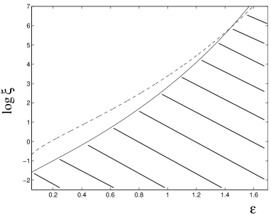
FIG. 1.: We compare the bound imposed by isotropy requirement at the BBN scale (Eq. (20)) with the one imposed by homogeneity at the same epoch (Eq. (19)). We see that the homogeneity requirement (shaded region) is more constraining then the one of isotropy. The plot is in the case $\Omega_{B}h^{2}_{100}=0.01$, $h_{100}=0.6$, $\sigma_{c}/T_{c}=70$.

A more conservative attitude is to derive bounds on the magnetic fields from the requirement that homogeneous BBN is not spoiled, i.e.

$$\Delta(L_{diff},t_{c})<\frac{n_{B}}{s}~{}.$$ (18)

In terms of $\xi$ and $\epsilon$ (which completely define our stochastic magnetic background) the bound (18) becomes

$$\log{\xi}<\frac{\log{\frac{\sigma_{c}}{T_{c}}}-6.26+\frac{1}{2}\log{\epsilon}+14.88~{}\epsilon+\log{[\Omega_{B}h^{2}_{100}]}}{4-\epsilon}~{}.$$ (19)

We plot it in Fig. 1 for a typical choice of the parameters and $0.05\raise 1.29167pt\hbox{$<$\kern-7.5pt\raise-4.73611pt\hbox{$\sim$}}\epsilon\raise 1.29167pt\hbox{$<$\kern-7.5pt\raise-4.73611pt\hbox{$\sim$}}1.6$ (for $\sigma_{c}/T_{c}\simeq 70-100$, $\Omega_{B}h^{2}_{100}\simeq 0.1-0.01$, $0.4<h_{100}<1$ this bound does not change significantly). The bound (19) is quite strong for blue spectra (i. e. $0<\epsilon<1$). For violet spectra ($\epsilon>1$ in Eq. (17)) the fluctuations turns out to be parametrically smaller than $(n_{B}/s)$ at the neutron diffusion scale and then practically unconstrained by BBN.

The bounds on ordinary magnetic fields at the nucleosynthesis epoch do also apply in our case. For example in [3] was obtained that in order to be compatible with the isotropic nucleosynthesis $H_{N}(t_{NS})<1\times~{}10^{11}~{}{\rm Gauss}$ at a temperature $T_{NS}\sim 10^{9}~{}^{0}{\rm K}$ which implies, at $T_{c}$ , $H_{N}(t_{c})<1.34~{}\times 10^{23}~{}{\rm Gauss}$. By now comparing the magnetic hypercharge density with this bound we get a further condition in our exclusion plot, namely:

$$\log{\xi}<\frac{(11.30-\frac{1}{2}\log{\frac{\sigma_{c}}{T_{c}}})\epsilon+\log{\epsilon}-0.2}{4-\epsilon}~{}.$$ (20)

This condition is reported in Fig. 1 (upper curve) and compared with the one of Eq. (19) (lower curve). According to Fig. 1 Eq. (20) could be satisfied without satisfying Eq. (19) for $\epsilon\raise 1.29167pt\hbox{$<$\kern-7.5pt\raise-4.73611pt\hbox{$\sim$}}1.4$. This implies that the bound we derived is more constraining (by two orders of magnitude for magnetic field at $\epsilon\ll 1$) than the bounds reported in [3].

We thank J. Cline, M. Joyce, H. Kurki-Suonio, and G. Veneziano for helpful discussions and comments.

REFERENCES

- [1] P. P. Kronberg, Rept. Prog. Phys. 57, 325 (1994).
- [2] Y. B. Zeldovich, A. A. Rusmaikin and D. D. Sokoloff ”Magnetic Fields in Astrophysics” (New York, Gordon and Breach, 1983).
- [3] G. Greenstein, Nature 223, 938 (1969); J. J. Matese and R. F. O’ Connel, Astrophys. J. 160, 451 (1970); D. Grasso and H. Rubinstein, Phys. Lett. B 77, (1996); B. Cheng et al., Phys. Rev. D 54, 4174 (1996); P. Kernan et al., Phys. Rev. D 54, 7207 (1996).
- [4] G. Sigl, A.V. Olinto and K. Jedamzik, Phys.Rev. D 55, 4582 (1997).
- [5] T. Vachaspati, Phys. Lett. B 265, 258 (1991); K. Enqvist, P. Olesen, Phys. Lett. B 319, 178 (1993); T. W. Kibble and A. Vilenkin, Phys. Rev. D 52, 679 (1995); G. Baym, D. Bodeker and L. McLerran Phys.Rev. D 53, 662 (1996).
- [6] M. Joyce and M. Shaposhnikov, Phys. Rev. Lett. 79, 1193 (1997).
- [7] M.S. Turner and L.M. Widrow, Phys. Rev. D 37, 2743 (1988); B. Ratra, Astrophys. J. Lett, 391, L1 (1992); A. Dolgov and J. Silk, Phys. Rev. D 47, 3144 (1993);
- [8] M. Gasperini, M. Giovannini and G. Veneziano, Phys. Rev. Lett. 75, 3796 (1995); Phys. Rev. D 52, 6651 (1995); D. Lemoine and M. Lemoine, Phys. Rev. D 52, 1955 (1995).
- [9] A.N. Redlich and L.C.R. Wijewardhana, Phys. Rev. Lett. 54, 970 (1985)
- [10] M. Joyce, T. Prokopec and N. Turok, Phys. Rev. D 53, 2930 (1996); G. Baym and H. Heiselberg, astro-ph/9704214
- [11] D. Biskamp “Nonlinear Magnetohydrodynamics” (Cambridge University Press, Cambridge 1994).
- [12] V. A. Kuzmin, V. A. Rubakov and M. E. Shaposhnikov, Phys. Lett. B 155, 36 (1985).
- [13] M. E. Shaposhnikov, JETP Lett. 44, 465 (1986); Nucl. Phys. B 287, 757 (1987).
- [14] K. Kajantie, M. Laine, K. Rummukainen and M. Shaposhnikov, Nucl. Phys. B 495, 413 (1997)
- [15] M. Carena, M. Quiros, C. E. M. Wagner, Phys. Lett. B 380, 81 (1996); M. Laine, Nucl. Phys. B 481, 43 (1996); J.M. Cline and K. Kainulainen, Nucl. Phys. B 482, 73 (1996); M. Losada, hep-ph/9605266.
- [16] J. Cline, K. Kainulainen and K. Olive, Phys. Rev. Lett. 71:2372, 1993; Phys. Rev. D 49, 6394 (1994).
- [17] M. Giovaninni and M. Shaposhnikov, in preparation.
- [18] If the spectrum is dominated by parity non-invariant configurations then, in general, . Examples of this types of configurations can be found in [6]. If this is the case, the baryon asymmetry of the universe can be a result of decay of Chern-Simons condensate [13].
- [19] J. Applegate, C. J. Hogan and R. J. Scherrer, Phys. Rev. D 35, 1151 (1987); B. Banerjee and S. M. Chitre, Phys. Lett. B 258, 247 (1991);K. Jedamzik and G. M. Fuller, Astrophys. J. 423, 33 (1994); K. Jedamzik and G. M. Fuller, Astrophys. J. 452, 33 (1995); H. Kurki-Suonio, K. Jedamzik and G. J. Mathews, astro-ph/9606011.