$\mbox{$B\rightarrow X_{q}l^{+}l^{-}$ }(q=d,s)$ and Determination of $\left|{V_{td}\over V_{ts}}\right|$

Abstract

We propose a new method to extract $|V_{td}|\over|V_{ts}|$ from the ratio of the decay distributions ${dR\over ds}\equiv\mbox{${d{\cal{B}}\over ds}[\mbox{$B\rightarrow X_{d}l^{+}l^{-}$}]$}/\mbox{${d{\cal{B}}\over ds}[\mbox{$B\rightarrow X_{s}l^{+}l^{-}$ }]$}$. This ratio depends only on the KM ratio ${|V_{td}|\over|V_{ts}|}$ with $15\%$ theoretical uncertainties, if dilepton invariant mass-squared $s$ is away from the peaks of the possible resonance states, $J/\psi$, $\psi^{\prime}$, and etc. We also give a detailed analytical and numerical analysis on $\mbox{${d{\cal{B}}\over ds}[\mbox{$B\rightarrow X_{q}l^{+}l^{-}$ }]$}(q=d,s)$ and ${dR\over ds}$.

1 Introduction

The determination of the elements of KM matrix is one of the most important issues in the quark flavor physics. Moreover, the element $V_{td}$ (or $V_{ub}$) is especially important to the Standard Model description of CP-violation. If it were zero, there would be no CP-violation from the KM matrix elements (i.e. within the Standard Model), and we have to seek for other source of CP violation in $K_{L}\rightarrow\pi\pi$. Here we study the ratio $V_{td}\over V_{ts}$. In the Standard Model with the unitarity of KM matrix, $V_{ts}$ is approximated by $-V_{cb}$, which is directly measured by semileptonic $B$ decays. There are already several ways to determine $V_{td}$ available in the literature:

• $|V_{td}|$ can be indirectly extracted through $B_{d}-\overline{B}_{d}$ mixing. However, in $B_{d}-\overline{B}_{d}$ mixing the large uncertainty of the hadronic matrix elements prevents us to extract the element of KM with good accuracy.

• A better extraction of $|{V_{td}\over V_{ts}}|$ can be made if $B_{s}-\overline{B}_{s}$ is measured as well, because the ratio $f_{{}_{B_{d}}}^{2}B_{{}_{B_{d}}}/f_{{}_{B_{s}}}^{2}B_{{}_{B_{s}}}$ can be much better determined.

• The determination of $|{V_{td}\over V_{ts}}|$ from the ratios of rates of several hadronic two-body $B$ decays, such as $\Gamma(B^{0}\to\overline{K}^{*0}K^{0})/\Gamma(B^{0}\to\phi K^{0})$, $\Gamma(B^{0}\to\overline{K}^{*0}K^{*0})/\Gamma(B^{0}\to\phi K^{*0})$, $\Gamma(B^{+}\to\overline{K}^{*0}K^{+})/\Gamma(B^{+}\to\phi K^{+})$, and $\Gamma(B^{+}\to\overline{K}^{*0}K^{*+})/\Gamma(B^{+}\to\phi K^{*+})$ has been also proposed in Ref. [1].

• $V_{td}$ can be determined from $K^{+}\to\pi^{+}\nu\bar{\nu}$ decay within $\sim 15\%$ theoretical uncertainties with the branching fraction ${\cal B}\sim 10^{-10}$ [2].

Why do we discuss yet another method to determine $V_{td}$? The main reason we are interested in $B$ physics is that this area is very likely to yield information about new physics beyond the Standard Model. We expect that new physics will influence experimentally measureable quantities in different ways. For example, most of us expect that $\Delta B=2$ transition is more sensitive to new physics than the decay rates. New physics may couple differently to $K$ mesons compared to $B$ mesons. Therefore, it is essential to determine the KM matrix elements in as many different methods as possible.

In this paper, we propose another method to determine ${|V_{td}|\over|V_{ts}|}$ precisely from the decay distributions ${d{\cal{B}}\over ds}[\mbox{$B\rightarrow X_{s}l^{+}l^{-}$ }]$ and ${d{\cal{B}}\over ds}[\mbox{$B\rightarrow X_{d}l^{+}l^{-}$}]$, where $s$ is invariant mass-squared of final lepton pair, $l^{+}l^{-}$. In the decays of $\mbox{$B\rightarrow X_{q}l^{+}l^{-}$ }(q=d,s)$, the short distance (SD) contribution comes from the top quark loop diagrams and the long distance (LD) contribution comes from the decay chains due to intermediate charmonium states. Therefore, the former (SD) amplitude is proportional to ${V_{tq}}^{*}V_{tb}$, and the latter (LD) proportional to ${V_{cq}}^{*}V_{cb}$. If the invariant mass-squared of $l^{+}l^{-}$ is away from the peaks of the charmoniuum resonances ($J/\psi$ and $\psi^{\prime}$), the SD contribution is dominant, while on the peaks of the resonances the LD contribution is dominant, and therefore we expect that in the $SU(3)$ symmetry limit the ratio

$${dR\over ds}\equiv{d{\cal{B}}\over ds}(B\rightarrow X_{d}l^{+}l^{-})/{d{\cal{B}}\over ds}(B\rightarrow X_{s}l^{+}l^{-})$$

becomes

$${1\over\lambda^{2}}{dR(s)\over ds} \rightarrow (1-\rho)^{2}+\eta^{2}\quad(s\rightarrow 1\rm{GeV}^{2})~{},$$ (1)

$$\rightarrow \qquad 1\qquad\qquad(s\rightarrow{m_{{}_{J/\psi}}}^{2})~{},$$

where $\lambda$ is $sin\theta_{c}$, $\theta_{c}$= Cabibbo angle, and for $\rho$, $\eta$, see Eq. (8). In the intermediate region, there is a characteristic interference beteen the LD contribution and the SD contribution, which requires the detailed study of the distributions. By focusing on the region, $1({\rm GeV}^{2})\leq s<m_{J/\psi}^{2}$, we can study $|{V_{td}\over V_{ts}}|$ from the experimental ratio of the distributions ${dR\over ds}$.

We stress the advantages to use the inclusive semileptonic decays:

• If dilepton invariant mass-squared $s$ is away from the peaks of the possible intermediate states, $J/\psi$, $\psi^{\prime}$, $\rho$, $\omega$, and etc., the short distance contribution due to top quark loop is dominant. Therefore, we may extract very precisely the combination of $|{V_{td}\over V_{ts}}|$ from the decay distributions within the range $1({\rm GeV}^{2})\leq s<{m_{J/\Psi}}^{2}$ without any theoretical uncertainties from the LD hadronic matrices, unknown KM matrix elements, and etc.

• Inclusive decay distributions are theoretically well predicted by heavy quark mass expansion away from the phase space boundary. The leading order of the expansion agrees with the parton model result. Furthermore, non-perturbative $1/{m_{b}}^{2}$ power corrections of QCD can be easily incorporated.

This paper is organized as follows. In Section 2, we present the analytic formulae for ${d{\cal{B}}\over ds}[\mbox{$B\rightarrow X_{s}l^{+}l^{-}$ }]$ and ${d{\cal{B}}\over ds}[\mbox{$B\rightarrow X_{d}l^{+}l^{-}$}]$. We also show in detail the decay distribution ${d{\cal{B}}\over ds}[\mbox{$B\rightarrow X_{s}l^{+}l^{-}$ }]$ including the uncertainties coming from top quark mass $m_{t}$ and the scale of renormalization group $\mu$. In Section 3, after brief discussion on the limit of KM elements coming from $B_{d}-\overline{B}_{d}$ mixing and $B\rightarrow X_{u}l\bar{\nu}$, we study the ratio of the decay distributions, and show how we may extract $|{V_{td}\over V_{ts}}|$.

2 Effective Hamiltonian for $b\rightarrow ql^{+}l^{-}$ and their differential decay rates.

In this Section, the differential decay rates for $\mbox{$B\rightarrow X_{q}l^{+}l^{-}$ }(q=d,s)$ are shown including both LD and SD effects as well as ${\Lambda_{QCD}}^{2}/{m_{b}}^{2}$ power corrections. (See [3] for $b\rightarrow dl^{+}l^{-}$, [4] for $b\rightarrow sl^{+}l^{-}$, and [5], [6] for $B\rightarrow X_{s}l^{+}l^{-}$ including the $1/{m_{b}}^{2}$ power corrections.) We also show in detail how the differential decay rate varies by changing the input parameters $m_{t}$, and the renormalization scale $\mu$. In Table 1, we summarize all the values of the input parameters used in our numerical calculations of decay rates. We use the central values for those input parameters, unless otherwise specified.

The effective Hamiltonian for $b\rightarrow ql^{+}l^{-}$ $(q=d,s)$ is given as

$${\cal H}_{eff} = -\frac{4G_{F}}{\sqrt{2}}V_{tq}^{*}V_{tb}\left[\sum_{i=1}^{10}C_{i}O_{i}\right]$$ (2)

$$+ \frac{4G_{F}}{\sqrt{2}}V_{uq}^{*}V_{ub}\left[C_{1}({O_{1}}^{u}-O_{1})+C_{2}({O_{2}}^{u}-O_{2})\right],$$

where $V_{ij}$ are the KM matrix elements. The operators are given as

$$O_{1} = (\bar{q}_{L\alpha}\gamma_{\mu}b_{L\alpha})(\bar{c}_{L\beta}\gamma^{\mu}c_{L\beta}),$$

$$O_{2} = (\bar{q}_{L\alpha}\gamma_{\mu}b_{L\beta})(\bar{c}_{L\beta}\gamma^{\mu}c_{L\alpha}),$$

$$O_{3} = (\bar{q}_{L\alpha}\gamma_{\mu}b_{L\alpha})\sum_{q^{\prime}=u,d,s,c,b}(\bar{q^{\prime}}_{L\beta}\gamma^{\mu}q^{\prime}_{L\beta}),$$

$$O_{4} = (\bar{q}_{L\alpha}\gamma_{\mu}b_{L\beta})\sum_{q^{\prime}=u,d,s,c,b}(\bar{q^{\prime}}_{L\beta}\gamma^{\mu}q^{\prime}_{L\alpha}),$$

$$O_{5} = (\bar{q}_{L\alpha}\gamma_{\mu}b_{L\alpha})\sum_{q^{\prime}=u,d,s,c,b}(\bar{q^{\prime}}_{R\beta}\gamma^{\mu}q^{\prime}_{R\beta}),$$

$$O_{6} = (\bar{q}_{L\alpha}\gamma_{\mu}b_{L\beta})\sum_{q^{\prime}=u,d,s,c,b}(\bar{q^{\prime}}_{R\beta}\gamma^{\mu}q^{\prime}_{R\alpha}),$$

$$O_{7} = \frac{e}{16\pi^{2}}\bar{q}_{\alpha}\sigma_{\mu\nu}(m_{b}R+m_{q}L)b_{\alpha}F^{\mu\nu},$$

$$O_{8} = \frac{g}{16\pi^{2}}\bar{q}_{\alpha}T_{\alpha\beta}^{a}\sigma_{\mu\nu}(m_{b}R+m_{q}L)b_{\beta}G^{a\mu\nu},$$

$${O_{1}}^{u} = (\bar{q}_{L\alpha}\gamma_{\mu}b_{L\alpha})(\bar{u}_{L\beta}\gamma^{\mu}u_{L\beta}),$$

$${O_{2}}^{u} = (\bar{q}_{L\alpha}\gamma_{\mu}b_{L\beta})(\bar{u}_{L\beta}\gamma^{\mu}u_{L\alpha}),$$

$$O_{9} = \frac{e^{2}}{16\pi^{2}}\bar{q}_{\alpha}\gamma^{\mu}Lb_{\alpha}\bar{l}\gamma_{\mu}l,$$

$$O_{10} = \frac{e^{2}}{16\pi^{2}}\bar{q}_{\alpha}\gamma^{\mu}Lb_{\alpha}\bar{l}\gamma_{\mu}\gamma_{5}l,$$ (3)

where $L$ and $R$ denote chiral projections, $L(R)=1/2(1\mp\gamma_{5})$. We use the Wilson coefficients given in the literature (see, for example, [7]).

With the effective Hamiltonian in Eq. (2), the matrix element for the decays $\mbox{$b\rightarrow ql^{+}l^{-}$ }(q=d,s)$ can be written as

$${\cal M(\mbox{$b\rightarrow ql^{+}l^{-}$ })} = \frac{G_{F}\alpha}{\sqrt{2}\pi}\,V_{tq}^{\ast}V_{tb}\,\left[\left(C_{9q}^{\mbox{eff}}-C_{10}\right)\left(\bar{q}\,\gamma_{\mu}\,L\,b\right)\left(\bar{l}\,\gamma^{\mu}\,L\,l\right)\right.$$ (4)

$$\left.\;\;\;\;\;\;\;\;\;\;\;\;\;\;\;\;\;\;+\left(C_{9q}^{\mbox{eff}}+C_{10}\right)\left(\bar{q}\,\gamma_{\mu}\,L\,b\right)\left(\bar{l}\,\gamma^{\mu}\,R\,l\right)\right.$$

$$\left.\;\;\;\;\;\;\;\;\;\;\;\;\;\;\;\;\;\;-2C_{7}^{\mbox{eff}}\left(\bar{q}\,i\,\sigma_{\mu\nu}\,\frac{q^{\nu}}{q^{2}}(m_{q}L+m_{b}R)\,b\right)\left(\bar{l}\,\gamma^{\mu}\,l\right)\right]\,,$$

where $C_{9q}^{\mbox{eff}}$ is given by

$$C_{9q}^{\mbox{eff}}(\hat{s})\equiv C_{9}\left\{1+\frac{\alpha_{s}(\mu)}{\pi}\omega(\hat{s})\right\}+{Y_{SD}}^{q}(\hat{s})+{Y_{LD}}^{q}(\hat{s})~{},$$ (5)

where $q^{\nu}$ is the four momentum of $l^{+}l^{-}$, $s=q^{2}$, and $\hat{s}=s/{m_{b}}^{2}$. The function ${Y_{SD}}^{q}(\hat{s})$ is the one-loop matrix element of $O_{9}$, and ${Y_{LD}}^{q}(\hat{s})$ is the LD contributions due to the vector mesons mesons $J/\psi$, $\psi^{\prime}$ and higher resonances. The function $\omega(\hat{s})$ represents the $O(\alpha_{s})$ correction from the one-gluon exchange in the matrix element of $O_{9}$, and is given in our Appendix. The two functions ${Y_{SD}}^{q}$ and ${Y_{LD}}^{q}$ are written as

$${Y_{SD}}^{q}(\hat{s}) = g(\hat{m}_{c},\hat{s})\left(3\,C_{1}+C_{2}+3\,C_{3}+C_{4}+3\,C_{5}+C_{6}\right)$$ (6)

$$-\frac{1}{2}g(1,\hat{s})\left(4\,C_{3}+4\,C_{4}+3\,C_{5}+C_{6}\right)$$

$$-\frac{1}{2}g(0,\hat{s})\left(C_{3}+3\,C_{4}\right)$$

$$+\frac{2}{9}\left(3\,C_{3}+C_{4}+3\,C_{5}+C_{6}\right)$$

$$-{V_{uq}^{*}V_{ub}\over V_{tq}^{*}V_{tb}}(3C_{1}+C_{2})(g(0,\hat{s})-g(\hat{m}_{c},\hat{s}))~{},$$

$${Y_{LD}}^{q}(\hat{s}) = \frac{3}{\alpha^{2}}\kappa\,\left(-{V_{cq}^{*}V_{cb}\over V_{tq}^{*}V_{tb}}C^{(0)}-{V_{uq}^{*}V_{ub}\over V_{tq}^{*}V_{tb}}(3\,C_{3}+C_{4}+3\,C_{5}+C_{6})\right)$$ (7)

$$\times\sum_{V_{i}=\psi(1s),...,\psi(6s)}\frac{\pi\,\Gamma(V_{i}\rightarrow l^{+}l^{-})\,M_{V_{i}}}{{M_{V_{i}}}^{2}-\hat{s}\,{m_{b}}^{2}-iM_{V_{i}}\Gamma_{V_{i}}}~{},$$

where the function $g(\hat{m_{c}}={m_{c}\over m_{b}},\hat{s})$, $g(1,\hat{s})$, and $g(0,\hat{s})$ represent $c$ quark, $b$ quark and $u,d,s$ quark loop contributions, respectively. The two functions $g(z,\hat{s})$ and $g(0,\hat{s})$ are given [7] in our Appendix. In Eq. (7), $C^{(0)}\equiv 3C_{1}+C_{2}+3C_{3}+C_{4}+3\,C_{5}+C_{6}$, and the first two terms are dominant, as can be seen from the Table $2$.

It is convenient to write the relevant combinations of KM in terms of the Wolfenstein parametrization. In the following, in addition to $A$ and $\lambda$, we choose $(1-\rho)^{2}+\eta^{2}$ and $\phi_{1}=arg(-{{V_{cd}V_{cb}^{*}}\over{V_{td}V_{tb}^{*}}})$ as independent variables, then we have

$$V_{ts}^{*}V_{tb} \simeq \lambda^{2}A~{},$$

$$\frac{V_{cs}^{*}V_{cb}}{V_{ts}^{*}V_{tb}} \simeq -1~{},$$

$$\frac{V_{us}^{*}V_{ub}}{V_{ts}^{*}V_{tb}} \simeq O(\lambda^{2})~{},$$

$$V_{td}^{*}V_{tb} \simeq \lambda^{3}A(1-\rho+i\eta)~{},$$

$$\frac{V_{cd}^{*}V_{cb}}{V_{td}^{*}V_{tb}} \simeq -\frac{1}{1-\rho+i\eta}~{},$$

$$= -\frac{\exp(-i\phi_{1})}{\sqrt{(1-\rho)^{2}+\eta^{2}}}~{},$$

$$\frac{V_{ud}^{*}V_{ub}}{V_{td}^{*}V_{tb}} \simeq \frac{\rho-i\eta}{1-\rho+i\eta}~{},$$ (8)

$$= -1+\frac{\exp(-i\phi_{1})}{\sqrt{(1-\rho)^{2}+\eta^{2}}}~{}.$$

In the SD contribution of $B\rightarrow X_{s}l^{+}l^{-}$ , the $u$-quark loop contribution is neglected due to the smallness of the combination $V_{us}^{*}V_{ub}$ compared with $V_{cs}^{*}V_{cb}\simeq-V_{ts}^{*}V_{tb}$, while in $B\rightarrow X_{d}l^{+}l^{-}$ the term which is proportional to $V_{ud}^{*}V_{ub}$ is maintained. In the LD contribution, there is a contribution coming from the gluonic penguin amplitude which is proportional to $\frac{V_{ud}^{*}V_{ub}}{V_{td}^{*}V_{tb}}(3C_{3}+C_{4}+3C_{5}+C_{6})$. This contribution is neglected because of the smallness of the Wilson coefficient $(3C_{3}+C_{4}+3C_{5}+C_{6})$ compared with $C^{(0)}$. We adopt $\kappa=2.3$ [8] to reproduce the rate of the decay chain $B\rightarrow X_{s}J/\psi\rightarrow X_{s}l^{+}l^{-}$. Note that the data determines only the combination, $\kappa\,C^{(0)}=0.88$.

By combining both SD and LD contributions as well as non-perturbative $1/{m_{b}}^{2}$ power corrections, the differential decay rate for $\mbox{$B\rightarrow X_{q}l^{+}l^{-}$ }(q=d,s)$ becomes

$$\frac{{\rm d}{\cal B}}{{\rm d}\hat{s}}=2\frac{{|V_{tq}^{*}V_{tb}|}^{2}}{\left|V_{cb}\right|^{2}}\;{\cal B}_{0}\left\{\left[\frac{2}{3}\hat{u}(\hat{s},\hat{m}_{q})((1-\hat{m}_{q}^{2})^{2}+\hat{s}(1+\hat{m}_{q}^{2})-2\hat{s}^{2})\right.\right.$$

$$+\frac{1}{3}(1-4\hat{m}_{q}^{2}+6\hat{m}_{q}^{4}-4\hat{m}_{q}^{6}+\hat{m}_{q}^{8}-\hat{s}+\hat{m}_{q}^{2}\hat{s}+\hat{m}_{q}^{4}\hat{s}-\hat{m}_{q}^{6}\hat{s}$$

$$-3\hat{s}^{2}-2\hat{m}_{q}^{2}\hat{s}^{2}-3\hat{m}_{q}^{4}\hat{s}^{2}+5\hat{s}^{3}+5\hat{m}_{q}^{2}\hat{s}^{3}-2\hat{s}^{4})\frac{\hat{\lambda}_{1}}{\hat{u}(\hat{s},\hat{m}_{q})}$$

$$+\left(1-8\hat{m}_{q}^{2}+18\hat{m}_{q}^{4}-16\hat{m}_{q}^{6}+5\hat{m}_{q}^{8}-\hat{s}-3\hat{m}_{q}^{2}\hat{s}+9\hat{m}_{q}^{4}\hat{s}-5\hat{m}_{q}^{6}\hat{s}-15\hat{s}^{2}\right.$$

$$\left.\left.-18\hat{m}_{q}^{2}\hat{s}^{2}-15\hat{m}_{q}^{4}\hat{s}^{2}+25\hat{s}^{3}+25\hat{m}_{q}^{2}\hat{s}^{3}-10\hat{s}^{4}\right)\frac{\hat{\lambda}_{2}}{\hat{u}(\hat{s},\hat{m}_{q})}\right]\left(|C_{9}^{\mbox{eff}}|^{2}+|C_{10}|^{2}\right)$$

$$+\left[\frac{8}{3}\hat{u}(\hat{s},\hat{m}_{q})\left(2(1+\hat{m}_{q}^{2})(1-\hat{m}_{q}^{2})^{2}-(1+14\hat{m}_{q}^{2}+\hat{m}_{q}^{4})\hat{s}-(1+\hat{m}_{q}^{2})\hat{s}^{2}\right)\right.$$

$$+\frac{4}{3}(2-6\hat{m}_{q}^{2}+4\hat{m}_{q}^{4}+4\hat{m}_{q}^{6}-6\hat{m}_{q}^{8}+2\hat{m}_{q}^{10}$$

$$-5\hat{s}-12\hat{m}_{q}^{2}\hat{s}+34\hat{m}_{q}^{4}\hat{s}-12\hat{m}_{q}^{6}\hat{s}-5\hat{m}_{q}^{8}\hat{s}+3\hat{s}^{2}$$

$$+29\hat{m}_{q}^{2}\hat{s}^{2}+29\hat{m}_{q}^{4}\hat{s}^{2}+3\hat{m}_{q}^{6}\hat{s}^{2}+\hat{s}^{3}-10\hat{m}_{q}^{2}\hat{s}^{3}+\hat{m}_{q}^{4}\hat{s}^{3}-\hat{s}^{4}-\hat{m}_{q}^{2}\hat{s}^{4})\frac{\hat{\lambda}_{1}}{\hat{u}(\hat{s},\hat{m}_{q})}$$

$$+4\left(-6+2\hat{m}_{q}^{2}+20\hat{m}_{q}^{4}-12\hat{m}_{q}^{6}-14\hat{m}_{q}^{8}+10\hat{m}_{q}^{10}+3\hat{s}+16\hat{m}_{q}^{2}\hat{s}+62\hat{m}_{q}^{4}\hat{s}\right.$$

$$-56\hat{m}_{q}^{6}\hat{s}-25\hat{m}_{q}^{8}\hat{s}+3\hat{s}^{2}+73\hat{m}_{q}^{2}\hat{s}^{2}+101\hat{m}_{q}^{4}\hat{s}^{2}+15\hat{m}_{q}^{6}\hat{s}^{2}+5\hat{s}^{3}-26\hat{m}_{q}^{2}\hat{s}^{3}+$$

$$\left.\left.5\hat{m}_{q}^{4}\hat{s}^{3}-5\hat{s}^{4}-5\hat{m}_{q}^{2}\hat{s}^{4}\right)\frac{\hat{\lambda}_{2}}{\hat{u}(\hat{s},\hat{m}_{q})}\right]\frac{|C_{7}^{\mbox{eff}}|^{2}}{\hat{s}}+\left[8\hat{u}(\hat{s},\hat{m}_{q})\left((1-\hat{m}_{q}^{2})^{2}\right.\right.$$

$$\left.-(1+\hat{m}_{q}^{2})\hat{s}\right)+4(1-2\hat{m}_{q}^{2}+\hat{m}_{q}^{4}-\hat{s}-\hat{m}_{q}^{2}\hat{s})\;\hat{u}(\hat{s},\hat{m}_{q})\;\hat{\lambda}_{1}$$

$$+4\left(-5+30\hat{m}_{q}^{4}-40\hat{m}_{q}^{6}+15\hat{m}_{q}^{8}-\hat{s}+21\hat{m}_{q}^{2}\hat{s}+25\hat{m}_{q}^{4}\hat{s}-45\hat{m}_{q}^{6}\hat{s}+13\hat{s}^{2}\right.$$

$$\left.\left.\left.+22\hat{m}_{q}^{2}\hat{s}^{2}+45\hat{m}_{q}^{4}\hat{s}^{2}-7\hat{s}^{3}-15\hat{m}_{q}^{2}\hat{s}^{3}\right)\frac{\hat{\lambda}_{2}}{\hat{u}(\hat{s},\hat{m}_{q})}\right]Re(C_{9}^{\mbox{eff}})\,C_{7}^{\mbox{eff}}\right\}\,.$$ (9)

We explain some aspect of the expression, (9):

• The branching ratio is normalized by ${\cal B}_{sl}$ of decays $B\to(X_{c},X_{u})l\nu_{l}$. We separate a combination of the KM factor $\frac{{|V_{tq}^{*}V_{tb}|}^{2}}{\left|V_{cb}\right|^{2}}$ due to top-quark loop from the normalization factor ${\cal B}_{0}$. The normalization constant ${\cal B}_{0}$ is

  $${\cal B}_{0}\equiv{\cal B}_{sl}\frac{3\,\alpha^{2}}{16\pi^{2}}\frac{1}{f(\hat{m}_{c})\kappa(\hat{m}_{c})}\,,$$ (10)

  where $f(\hat{m}_{c})$ is a phase space factor, and $\kappa(\hat{m}_{c})$ accounts for both the $O(\alpha_{s})$ QCD correction to the semi-leptonic decay width and the leading order $(1/m_{b})^{2}$ power correction, They are given in our Appendix explicitly.

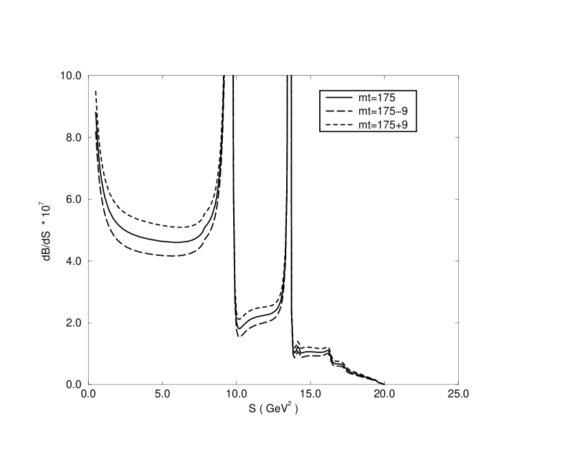
Figure 1: Dilepton invariant mass spectrum, ${{\rm d}{\cal B}\over{\rm d}s}(B\to X_{s}e^{+}e^{-})\times 10^{7}$. The unit of $s$ is ${\rm(GeV^{2})}$. The solid line corresponds to $m_{t}=175~{}(\rm{GeV})$. The short-dashed line corresponds to $m_{t}=175+9$. The long-dashed line corresponds to $m_{t}=175-9.$

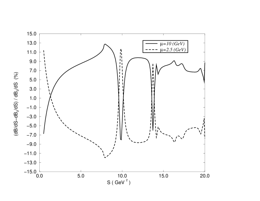
Figure 2: The $\%$ variation of dilepton invariant mass spectrum defined as $({{\rm d}{\cal B}(\mu)\over{\rm d}s}-{{\rm d}{\cal B}_{0}\over{\rm d}s})/{{\rm d}{\cal B}_{0}\over{\rm d}s}$; ${\cal B}_{0}={\cal B}(\mu=5\mbox{(GeV)}$). The solid line corresponds to $\mu=10$ and the dashed line corresponds to $\mu=2.5.$

• The Wilson coefficients depend on the top quark mass $m_{t}$, the renormalization scale $\mu$, and $\Lambda_{QCD}$. Their dependences are studied in Tables 2, 3 and 4. As the value of $\mu$ ($\Lambda_{QCD}$) decreases (increases) , $|C_{7}|$ and $C_{9}$ are getting larger, while $C_{10}$ is independent on $\mu$. As $m_{t}$ increases, $|C_{7}|$, $C_{9}$ and $|C_{10}|$ all become larger. The matrix elements also depend on the renormalization scale $\mu$, and their dependence is partially cancelled by the given dependence of the Wilson coefficients. The overall dependence can be studied with the differential rate. In Figs. 1 and 2, we show the dependence of the differential rate on $m_{t}$ and $\mu$. As the value of $m_{t}$ increases from 166 (GeV) to 184 (GeV), the differential rate increases about $20\%$ at $s\sim 5$ (GeV²), as shown in Fig. 1. At around the same region of $s$, by changing $\mu$ from 2.5 (GeV) to 10 (GeV) the differential rate increases about $20\%$, as shown in Fig. 2. This observation is consistent with the result of Ref. [7], in which only the SD contribution has been analysed.

• The differential decay rate (9) is not a simple parton model result. It contains non-perturbative $1/{m_{b}}^{2}$ power corrections, which are denoted in Eq. (9) by the terms proportional to $\hat{\lambda}_{1}$ and $\hat{\lambda}_{2}$. The parameters $\hat{\lambda}_{1}$ and $\hat{\lambda}_{2}$ are related to the matrix elements of the higher derivative operators of heavy quark effective theory [5], [9];

  $$\left<B\left|\bar{h}\,(i\,D)^{2}\,h\right|B\right> \equiv 2\,M_{B}\,\lambda_{1}=2M_{B}{m_{b}}^{2}\hat{\lambda}_{1}\,,$$

  $$\left<B\left|\bar{h}\,\frac{-i}{2}\sigma^{\mu\nu}\,G_{\mu\nu}\,h\right|B\right> \equiv 6\,M_{B}\,\lambda_{2}=6M_{B}{m_{b}}^{2}\hat{\lambda}_{2}\,,$$ (11)

  where $B$ denotes the pseudoscalar $B$ meson, $D_{\mu}$ is the covariant derivative, and $G_{\mu\nu}$ is the QCD field strength tensor.

3 The extraction of $\left|{V_{td}\over V_{ts}}\right|$

Presently we can constrain the value of $(1-\rho)^{2}+\eta^{2}$ from $B_{d}-\overline{B}_{d}$ mixing, while from $B\rightarrow X_{u}l\bar{\nu}$ we obtain some limit on $\rho^{2}+\eta^{2}$. Using those given limits, we can show how the ratio ${1\over\lambda^{2}}{dR\over ds}$ depends on input KM values, $(1-\rho)^{2}+\eta^{2}$ and $\phi_{1}~{}({\rm or}~{}\beta)$.

As is well known, $|V_{tb}^{*}V_{td}|$ are written with $\Delta M_{d}$ of $B_{d}-\overline{B}_{d}$ mixing. It reads as

$$|V_{tb}^{*}V_{td}| = A\lambda^{3}\sqrt{(1-\rho)^{2}+\eta^{2}}$$ (12)

$$= \left[\frac{6\pi^{2}}{G_{F}^{2}\eta_{{}_{QCD}}M_{W}^{2}M_{B}}\right]^{1/2}\left[\frac{{\Delta{M_{d}}}^{1/2}}{B_{{}_{B_{d}}}^{1/2}f_{{}_{B_{d}}}|E(x_{t})|^{1/2}}\right],$$

where $E(x_{t})$ is the Inami-Lim function [10] of the box diagram, and $x_{t}\equiv\frac{{m_{t}}^{2}}{{m_{W}}^{2}}$. It has the value $|E(x_{t})|=2.58$ for $m_{t}=175$ (GeV) and it varies from $2.38$ to $2.78$ as $m_{t}$ varies from $166$ (GeV) to $184$ (GeV). We use the following values; $\eta_{{}_{QCD}}=0.55$, $m_{t}=175$ (GeV), and the experimental constraints

$$\Delta M_{d} = 0.474\pm 0.031(ps^{-1})~{},$$

$$\left|{V_{ub}\over V_{cb}}\right| = \lambda\sqrt{\rho^{2}+\eta^{2}}=0.08\pm 0.02~{}.$$ (13)

Then, those constraints (13) are translated into the limits of $(1-\rho)^{2}+\eta^{2}$ and $\sqrt{\rho^{2}+\eta^{2}}$ as

$$(1-\rho)^{2}+\eta^{2} = 0.85(1\pm 0.15)\left\{0.2/(B_{{}_{B_{d}}}^{1/2}f_{{}_{B_{d}}}({\rm GeV}))\right\}^{2}$$

$$= [0.59\pm 0.09,1.3\pm 0.20]~{},$$

$$\sqrt{\rho^{2}+\eta^{2}} = 0.36\pm 0.09~{}.$$ (14)

Here we used $B_{{}_{B_{d}}}^{1/2}f_{{}_{B_{d}}}=0.2\pm 0.04(\rm{GeV})$ to get the range of $(1-\rho)^{2}+\eta^{2}\approx[0.5,1.5]$. We also used $A\lambda^{2}=0.041(\pm 0.003)$, and $\lambda=0.2205$. In Fig. 3, we show the present limit in the plane of $(\phi_{1},~{}(1-\rho)^{2}+\eta^{2})$. The horizontal axis corresponds to $\phi_{1}~{}({\rm or}~{}\beta)$, and the unit is degree. The vertical axis corresponds to $(1-\rho)^{2}+\eta^{2}$. The thin dashed line is obtained from the central values of $|V_{ub}|$ and the thin solid line is obtained from $|V_{td}|$. The central value corresponds to $(\phi_{1},~{}(1-\rho)^{2}+\eta^{2})\approx(20^{o},~{}0.85)$.

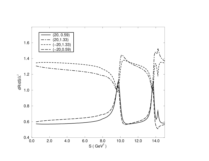
Figure 4: The ratio ${1\over\lambda^{2}}{dR\over ds}$ versus $s$ (GeV²) with two different input values of $(1-\rho)^{2}+\eta^{2}$. The solid curve correspond to $(\phi_{1},~{}(1-\rho)^{2}+\eta^{2})=(20^{o},~{}0.59)$, and the dot-dashed curve corresponds to $(20^{o},~{}1.33)$. The ratios for CP conjugate process ${\overline{B}}\rightarrow{\bar{X}_{q}}l^{+}l^{-}$ are denoted by the dashed curve for $(1-\rho)^{2}+\eta^{2}=1.33$, and by the long-dashed curve for $(1-\rho)^{2}+\eta^{2}=0.59$. They are obtained by reversing the sign of $\phi_{1}$ in the corresponding $B\rightarrow X_{q}l^{+}l^{-}$ process; $i.e.$, $\phi_{1}\rightarrow-\phi_{1}$.

Now let us consider the ratio ${1\over\lambda^{2}}{dR(s)\over ds}$. In the SU(3) limit, we expect that this ratio approaches to the input value of $(1-\rho)^{2}+\eta^{2}$ for the dileptonic invariant mass-squared $s$ far below the peak of charmonium resonances. If $s$ is on the peak of resonances, the ratio becomes 1. In Fig. 4, we show the ratio ${1\over\lambda^{2}}{dR(s)\over ds}$ for two sets of the assumed input values of $(\phi_{1},~{}(1-\rho)^{2}+\eta^{2})$, one of whose $(1-\rho)^{2}+\eta^{2}$ is 0.59, and the other is 1.33. They correspond to their small (or large) values allowed from the present experimental result of $B_{d}-\overline{B}_{d}$ mixing. The solid curve corresponds to $(\phi_{1},~{}(1-\rho)^{2}+\eta^{2})=(20^{o},~{}0.59)$, and the dot-dashed curve corresponds to $(20^{o},~{}1.33)$. The ratios for the CP conjugate process ${\overline{B}}\rightarrow{\bar{X}_{q}}l^{+}l^{-}$ are also shown, denoted by the long-dashed curve for $(1-\rho)^{2}+\eta^{2}=1.33$, and by the dashed curve for $(1-\rho)^{2}+\eta^{2}=0.59$. They are obtained by reversing the sign of $\phi_{1}$ in the corresponding $B\rightarrow X_{q}l^{+}l^{-}$ process; i.e., $\phi_{1}\rightarrow-\phi_{1}$. They are labeled as $(-20^{o},~{}1.33)$ and $(-20^{o},~{}0.59)$ in Figure 4.

To summarize the numerical results of Fig. 4 and Section 3:

• The predicted ratio at low invariant mass region $s\simeq 1$ (GeV²) is very near to the our assumed input value of $(1-\rho)^{2}+\eta^{2}$, while on the peak of the resonances $J/\psi$, $\psi^{\prime}$, this ratio becomes almost 1, as we expected, i.e.

  $${1\over\lambda^{2}}{dR(s)\over ds} \rightarrow \quad\quad 1\quad\quad\quad\quad(s\sim{m_{J/\psi}}^{2},{m_{\psi^{\prime}}}^{2},..)~{},$$ (15)

  $$\rightarrow (1-\rho)^{2}+\eta^{2}\quad(s~{}~{}{\rm being~{}away~{}from}~{}{m_{J/\psi}}^{2},..)~{}.$$

• In the intermediate region, there is a characteristic interference between the LD contribution and the SD contribution, which can be only derived from the detailed expression of the distributions, Eq. (9).

• The value of the ratio does not depend much on whether the decaying particles are $B$ or $\overline{B}$ at any invariant mass-squared region.

• This ratio changes only a few $\%$ when we change the input parameters, $m_{t}$ and $\mu$, within the range shown in Table 1. The dependences on $m_{t}$ and $\mu$ are almost cancelled away in the ratio. Therefore, the uncertainties in this ratio due to the input parameters are much smaller than the uncertainties in the differential decay rate itself, as shown in Tables 2, 3 and 4 as well as in Figures 1 and 2.

• In Fig. 4 the range between the dot-dashed curve and the solid curve corresponds to the value of the ratio ${1\over\lambda^{2}}{dR(s)\over ds}$ allowed from the present experimental result of $B_{d}-\overline{B}_{d}$ mixing. Future experimental measurements on the ratio of the branching fractions, ${\cal B}(B\rightarrow X_{d}l^{+}l^{-})$ and ${\cal B}(B\rightarrow X_{s}l^{+}l^{-})$, can give much better alternative for determination of $|{V_{td}\over V_{ts}}|$ without any hadronic uncertainties, limited only by experimental statistics.

• If $10^{9}$ $B\overline{B}$ pairs are produced, the expected number of the events for $B\rightarrow X_{d}l^{+}l^{-}$ in the range of $4{m_{\mu}}^{2}<s<6$ GeV (${m_{\mu}}=$ muon mass) is about $100$ for $(1-\rho)^{2}+\eta^{2}=0.59$, and is about $220$ for $(1-\rho)^{2}+\eta^{2}=1.33$. Therefore, the statistical accuracy of $(1-\rho)^{2}+\eta^{2}$ determined from this method is about $7\%\sim 10\%$ with the expected production of $10^{9}$ $B\overline{B}$ pairs.

• We have assumed in our numerical analysis the flavor $SU(3)$ symmetry with $m_{d}=m_{s}$. We estimated the corrections due to $SU(3)$ breaking by varying $m_{d}$ from 0.01 GeV up to $m_{s}=0.2$ GeV. And we find the ratio ${dR\over ds}$ decreases within $0.2\sim 0.3\%$ for the range $1<s<9$ (GeV²). Therefore, we conclude the $SU(3)$ breaking effect does not affect the extraction of $|{V_{td}\over V_{ts}}|$ at all.

Acknowledgements

TM would like to thank G. Hiller, K. Ochi, T. Nasuno , and Y. Kiyo for correspondence and assistance of numerical computations. The preliminary version of this work was given [11] as a talk by TM at BCONF97, Hawaii, March 1997. The work of CSK was supported in part by the CTP, Seoul National University, in part by the BSRI Program, Ministry of Education, Project No. BSRI-97-2425, and in part by the KOSEF-DFG large collaboration project, Project No. 96-0702-01-01-2. The work of TM was partially supported by Monbusho International Scientific Research Program (No. $08044089$), and that of AIS and TM was supported also by Grant-in-Aid for Scientific Research on Priorty Areas (Physics of CP violation) from the Ministry of Education and Culture of Japan .

Parameter	Value
$m_{W}$	$80.26$ (GeV)
$m_{Z}$	$91.19$ (GeV)
$\sin^{2}\theta_{W}$	$0.2325$
$m_{s}$	$0.2$ (GeV)
$m_{d}$	$0.01$ (GeV)
$m_{c}$	$1.4$ (GeV)
$m_{b}$	$4.8$ (GeV)
$m_{t}$	$175\pm 9$ (GeV)
$\mu$	$5^{+5.0}_{-2.5}$ (GeV)
$\Lambda_{QCD}^{(5)}$	$0.214^{+0.066}_{-0.054}$ (GeV)
$\alpha_{QED}^{-1}$	129
$\alpha_{s}(m_{Z})$	$0.117\pm 0.005$
${\cal B}_{sl}$	$(10.4\pm 0.4)$ %
$\lambda_{1}$	$-0.20$ (GeV2)
$\lambda_{2}$	$+0.12$ (GeV2)

Table 1: Values of the input parameters used in the numerical calculations of the decay rates. Unless, otherwise specified, we use the central values.

$\mu$	$C_{1}$	$C_{2}$	$C_{3}$	$C_{4}$	$C_{5}$	$C_{6}$	$C_{7}^{\mbox{eff}}$	$C_{9}^{NDR}$	$C^{(0)}$
5	-0.2404	1.1031	0.0107	-0.0249	0.0072	-0.0302	-0.3110	4.1530	0.3805
10	-0.1606	1.0642	0.0068	-0.0170	0.0051	-0.0194	-0.2768	3.7551	0.5816
2.5	-0.3472	1.1614	0.0163	-0.0348	0.0096	-0.0462	-0.3525	4.4128	0.1163

Table 2: $\mu$ (in GeV) dependence of the Wilson coefficients used in the numerical calculations. The values of $\Lambda_{QCD}$ and $m_{t}$ are fixed at their central values.

${\Lambda_{QCD}}^{5}$	$C_{1}$	$C_{2}$	$C_{3}$	$C_{4}$	$C_{5}$	$C_{6}$	$C_{7}^{\mbox{eff}}$	$C_{9}^{NDR}$	$C^{(0)}$
0.214	-0.2404	1.1031	0.0107	-0.0249	0.0072	-0.0302	-0.3110	4.1530	0.3805
0.280	-0.2579	1.1122	0.0116	-0.0265	0.0076	-0.0327	-0.3181	4.2137	0.3369
0.160	-0.2242	1.0949	0.0099	-0.0233	0.0068	-0.0279	-0.3043	4.0891	0.4212

Table 3: ${\Lambda_{QCD}}^{5}$ dependence of the Wilson coefficients used in the numerical calculations. The values of $m_{t}$ and $\mu$ are fixed at their central values.

$m_{t}$	$C_{7}^{\mbox{eff}}$	$C_{9}^{NDR}$	$C_{10}$
$175$	$-0.311$	$4.153$	$-4.546$
$166$	$-0.3066$	$4.0796$	$-4.1877$
$184$	$-0.3150$	$4.2238$	$-4.9156$

Table 4: $m_{t}$ dependence of the Wilson coefficients used in the numerical calculations. The values of ${\Lambda_{QCD}}^{5}$ and $\mu$ are fixed at their central values.

Appendix

Appendix A Functions $g(z,\hat{s})$, $g(0,\hat{s})$ and $\omega(\hat{s})$

The functions $g(z,\hat{s})$ and $g(0,\hat{s})$ are given as

$$g(z,\hat{s}) = -\frac{8}{9}\ln(\frac{m_{b}}{\mu})-\frac{8}{9}\ln z+\frac{8}{27}+\frac{4}{9}y-\frac{2}{9}(2+y)\sqrt{|1-y|}$$ (16)

$$\times \left[\Theta(1-y)(\ln\frac{1+\sqrt{1-y}}{1-\sqrt{1-y}}-i\pi)+\Theta(y-1)2\arctan\frac{1}{\sqrt{y-1}}\right],$$

with $y=4z^{2}/\hat{s}$, and

$$g(0,\hat{s})=\frac{8}{27}-\frac{8}{9}\ln(\frac{m_{b}}{\mu})-\frac{4}{9}\ln\hat{s}+\frac{4}{9}i\pi~{}.$$ (17)

The function $\omega(\hat{s})$ represents the $O(\alpha_{s})$ correction from the one-gluon exchange in the matrix element of $O_{9}$ [12];

$$\omega(\hat{s}) = -\frac{2}{9}\pi^{2}-\frac{4}{3}{\mbox{L}i}_{2}(\hat{s})-\frac{2}{3}\ln\hat{s}\ln(1-\hat{s})-\frac{5+4\hat{s}}{3(1+2\hat{s})}\ln(1-\hat{s})$$ (18)

$$- \frac{2\hat{s}(1+\hat{s})(1-2\hat{s})}{3(1-\hat{s})^{2}(1+2\hat{s})}\ln\hat{s}+\frac{5+9\hat{s}-6\hat{s}^{2}}{6(1-\hat{s})(1+2\hat{s})}~{}.$$

Appendix B Functions $f(\hat{m}_{c})$ and $\kappa(\hat{m}_{c})$

The phase space function for $\Gamma(B\rightarrow X_{c}l\nu)$ in the lowest order (i.e., parton model)

$$f(\hat{m}_{c})=1-8\,\hat{m}_{c}^{2}+8\,\hat{m}_{c}^{6}-\hat{m}_{c}^{8}-24\,\hat{m}_{c}^{4}\,\ln\hat{m}_{c}~{}.$$ (19)

And $\kappa(\hat{m}_{c})$ accounts for both the $O(\alpha_{s})$ QCD correction to the semi-leptonic decay width and the leading order $(1/m_{b})^{2}$ power correction,

$$\kappa(\hat{m}_{c})=1-\frac{2\alpha_{s}(m_{b})}{3\pi}g(\hat{m}_{c})+\frac{h(\hat{m}_{c})}{2m_{b}^{2}}~{}.$$ (20)

The function $g(\hat{m}_{c})$ is given [12],[13] as

$$g(\hat{m}_{c})=(\pi^{2}-\frac{31}{4})(1-\hat{m}_{c})^{2}+\frac{3}{2}~{},$$ (21)

and finally the function $h(\hat{m}_{c})$ is given [9] as

$$h(\hat{m}_{c})=\lambda_{1}+\frac{\lambda_{2}}{f(\hat{m}_{c})}\left[-9+24\hat{m}_{c}^{2}-72\hat{m}_{c}^{4}+72\hat{m}_{c}^{6}-15\hat{m}_{c}^{8}-72\hat{m}_{c}^{4}\ln\hat{m}_{c}\right],$$ (22)

where $\lambda_{1}~{}({\rm or}~{}-\mu_{\pi}^{2})$ and $\lambda_{2}~{}({\rm or}~{}\mu_{{}_{G}}^{2})$ denote the matrix element of the higher derivative operators of heavy quark effective theory, as defined in Eq. (11).

Figure 3: The limit on $(1-\rho)^{2}+\eta^{2}$ and $\phi_{1}~{}({\rm or}~{}\beta)$. The horizontal axis corresponds to $\phi_{1}$, and the unit is degree. The vertical axis corresponds to $(1-\rho)^{2}+\eta^{2}$. The thin dashed line and the thin solid line are obtained from the central values of $|V_{ub}|$ and $|V_{td}|$ respectively. The thick solid lines are obtained from the allowed range of $|V_{td}|$ from $B_{d}\bar{B_{d}}$ mixing. The thick dashed lines are obtained from the allowed range of $|V_{ub}|$.

References

[1]
M. Gronau and J.L. Rosner,
Phys. Lett. B376 (1996) 205.
[2]
G. Buchalla and A.J. Buras, Phys. Rev. D54 (1996) 6782.
[3]
F. Krüger and L.M. Sehgal,
Phys. Rev. D55 (1997) 2799.
[4]
C.S. Lim, T. Morozumi and A.I. Sanda,
Phys. Lett. B218 (1989) 343;
N.G. Deshpande, J. Trampetic and K. Panose,
Phys. Rev. D39 (1989) 1461;
P.J. O’Donnell and H.K.K. Tung,
Phys. Rev. D43 (1991) R2067;
A. Ali, T. Mannel and T. Morozumi,
Phys. Lett. B273 (1991) 505;
N. Paver and Riazuddin,
Phys. Rev. D45 (1992) 978.
[5]
A. Falk, M. Luke, and M.J. Savage,
Phys. Rev. D49 (1994) 3367.
[6]
A. Ali, G. Hiller, L. Handoko, and T.
Morozumi, Phys. Rev. D55 (1997) 4105.
[7]
A.J. Buras and M. Münz, Phys. Rev. D52
(1995) 186, and references therein.
[8]
Z. Ligeti and M.B. Wise, Phys. Rev. D53 (1996) 4937.
[9]
I.I. Bigi, M.A. Shifman, N.G. Uraltsev and
A.I. Vainshtein, Phys. Rev. Lett. 71 (1993) 496;
A.V. Manohar and M.B. Wise, Phys. Rev. D49 (1994) 1310;
B. Blok, L. Koyrakh, M. Shifman and A.I. Vainshtein,
Phys. Rev. D49 (1994) 335;
T. Mannel, Nucl. Phys. B423 (1994) 396;
M. Neubert, Phys. Rev. D49 (1994) 3392.
[10]
T. Inami and C.S. Lim,
Prog. Theor. Phys. 65 (1981) 297
[E. 65 (1981) 1772].
[11]
C.S. Kim, T. Morozumi and A.I. Sanda,
talk given at BCONF97, Hawaii, March 1997,
hep-ph/9706380 (June 1997).
[12]
M. Jeabek and J. H. Kühn,
Nucl. Phys. B320 (1989) 20.
[13]
C.S. Kim and A.D. Martin,
Phys. Lett. B225 (1989) 186;
A. Ali and E. Pietarinen,
Nucl. Phys. B154 (1979) 519;
N. Cabibbo, G. Corbò and L. Maiani,
Nucl. Phys. B155 (1979) 93.